Advances in Machine Learning Detecting Changeover Processes in Cyber Physical Production Systems

Abstract

The performance indicator, Overall Equipment Effectiveness (OEE), is one of the most important ones for production control, as it merges information of equipment usage, process yield, and product quality. The determination of the OEE is oftentimes not transparent in companies, due to the heterogeneous data sources and manual interference. Furthermore, there is a difference in present guidelines to calculate the OEE. Due to a big amount of sensor data in Cyber Physical Production Systems, Machine Learning methods can be used in order to detect several elements of the OEE by a trained model. Changeover time is one crucial aspect influencing the OEE, as it adds no value to the product. Furthermore, changeover processes are fulfilled manually and vary from worker to worker. They always have their own procedure to conduct a changeover of a machine for a new product or production lot. Hence, the changeover time as well as the process itself vary. Thus, a new Machine Learning based concept for identification and characterization of machine set-up actions is presented. Here, the issue to be dealt with is the necessity of human and machine interaction to fulfill the entire machine set-up process. Because of this, the paper shows the use case in a real production scenario of a small to medium size company (SME), the derived data set, promising Machine Learning algorithms, as well as the results of the implemented Machine Learning model to classify machine set-up actions.

1. Introduction

With a turnover of 103 billion euros, the metal industry is one of the largest German industrial sectors, which is characterized by volatile market conditions and a high level of competition [1,2]. Small and medium manufacturing companies (SMEs) see increasingly serious problems in meeting delivery deadlines and throughput times [3]. Apart from commercial planning systems for generating production plans, companies continue to use Excel (31%) and manual processes (10%) as a basis for planning [4]. The same is valid for machine changeover processes. Consequently, it is essential to ensure the profitability of a production company by means of efficient production planning and control and the resulting high level of responsiveness and flexibility. It is necessary to optimally align production planning with market and customer requirements and maintain plant efficiency at a high and stable level [5]. Here, the acquisition of real-time data provides an adequate response to the requirements and great potential for production planning and control in order to optimize the scheduling and coordination of work orders, as well as to react immediately to disturbance variables or unforeseen deviations from the plan [4,6]. In addition, transparency and improvement of human decision-making processes is necessary and can be provided by data driven methods [7].

An approach for optimizing the production outcome can be realized by increasing plant productivity itself. For this purpose, the availability of the plants must be increased by localizing and reducing different types of losses. The changeover processes contribute highly negative the availability of a production line as they add no value. Cyber Physical Production Systems (CPPS) can contribute to the aim of increasing OEE by the intelligent utilization of sensor data for modern techniques as Machine Learning (ML) in a manufacturing environment. In this research, we focus on the detection of changeover processes as one element of availability.

The OBerA project (OBerA: “Optimization of processes and machine tools through provision, analysis and target/actual comparison of production data”) was established to support metalworking companies from the SME sector in the digitalization of their system landscape. The project consortium consists out of five production-oriented companies from the region of Franconia in northern Bavaria, Siemens as technology partner and the University of Applied Sciences Würzburg-Schweinfurt as an academic partner.

Table 1. Production oriented partners of the OBerA consortium.

Company	Turnover (Mio. €)	Number of Employees	Industrial Sector	Production Characteristic
Brehm	10–50	100	Medical implants	Single part production, series production
Franken	10–50	200	Tools for drilling, milling, and thread cutting	Small series and series production
Kritzner	10–50	100	Automation and automotive	Single part production, small series production
Pabst	6–10	60	Automotive and aerospace	Single part production, small series production
Siemens	>600	3000	Electronic motors	Series production

shows the production companies of the OBerA project, which are small and medium size enterprises (SME) from the region of northern Bavaria from different industrial sectors. The intention was to cover a broad spectrum of different companies standing exemplarily for the region of northern Bavaria.

In the beginning of the project for each SME from Table 1, use cases were identified in workshops with all partners. It was defined that:

• every company has at least one use case,
• use cases must have a financial benefit,
• use cases must be implemented within the project runtime, and the learnings of the implementation are shared in dedicated workgroups.

Table 2. Use cases of the partners of the OBerA consortium.

Focus Topic	Company	Use Case
Changeover	Pabst	Detection of changeover phases, Changeover status monitor
	Siemens	ERP-based duration analytics tool for historic changeover times from past orders
Production planning	Brehm, Franken	Optimized sequencing of orders
	Brehm, Franken, Kritzner, Siemens	Online transparency of machine states
	Siemens	Operating of multiple machines with an operator guidance system
Tool management	Brehm, Franken, Kritzner, Siemens	Tool wear detection
	Brehm, Kritzner	Selection of tool management software

shows the defined use cases of the project OBerA. The three focus topics changeover, production planning, and tool management were identified and corresponding use cases were derived. Developments for the use case of the company Pabst for the “Detection of changeover phases” will be presented in this article.

A major goal of the project OBerA is to establish real-time data transparency in order to facilitate deviation management to increase productivity. To achieve this, availability management for the production facilities needs to be improved. Especially, this project aim arises from the boundary conditions of SMEs, as they must be very flexible and at the same time efficient in their value adding chain. Hence, the OEE is a reasonable indicator for controlling the productivity, but sufficient data needs to be derived for its calculation. Further, OEE is highly influenced by changeover processes, which is according to Table 2 one of the focus topics for the OBerA SMEs. Related to their production characteristics (see Table 1, right most column), the product variety is high, as well as the complexity of the manufactured parts.

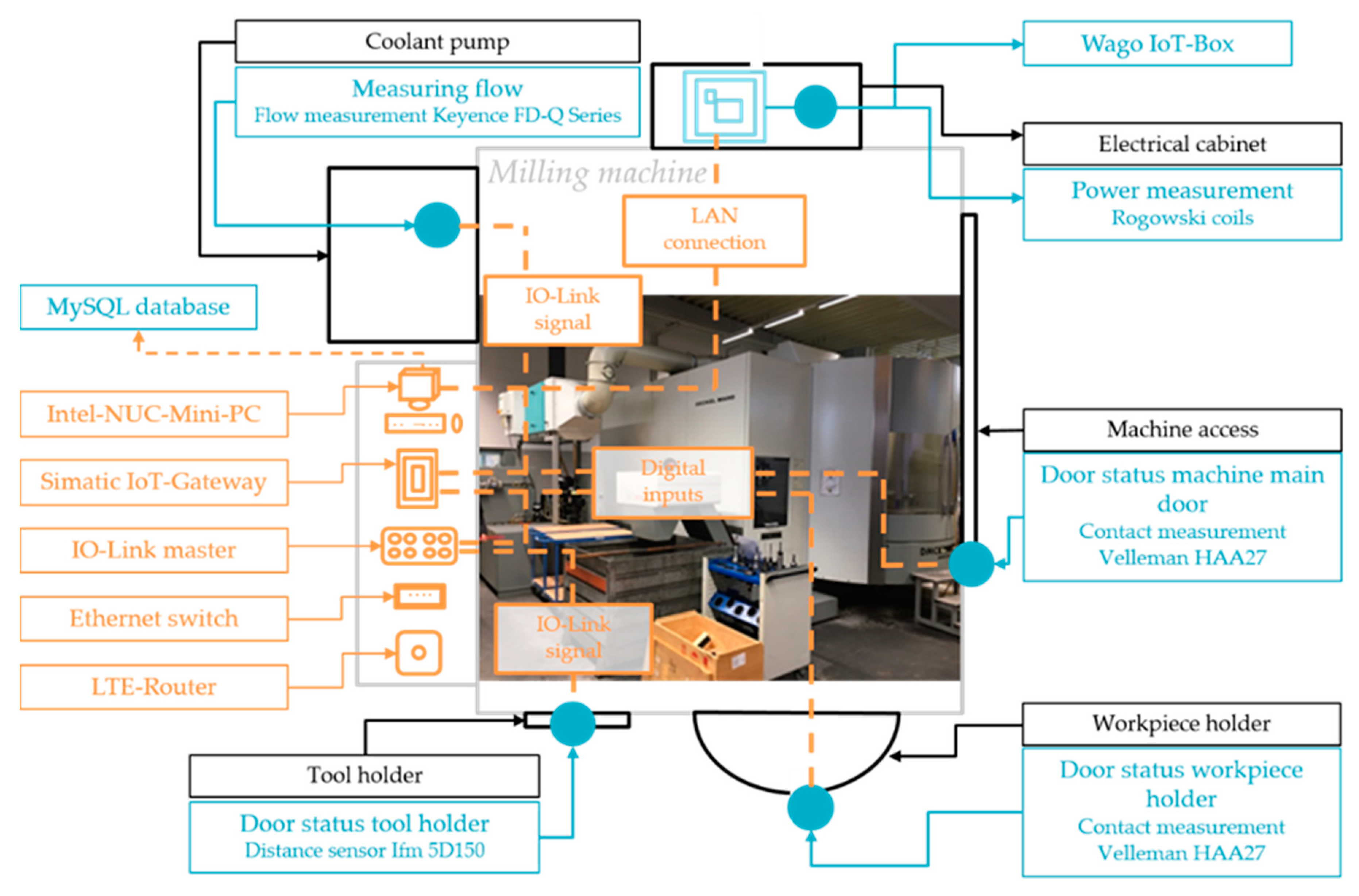
In this context, Yazdi et al. [8] investigate the relationship of OEE and manufacturing sustainability by a time-series analysis of a lab material handling system with conveyor belts and a robotic arm. In their research, they indexed value-adding and non-value-adding sub processes by video analysis to derive the OEE. In an extended research, the same research group [9] creates a simulation model to pre-analyze potential OEE improvements, before implementing them in the lab system. In addition to this research, we want to apply Machine Learning techniques to identify heterogeneous changeover processes (human and machine involvement) as the main research objective in this contribution. In the presented use case, the Pabst GmbH company produces mechanical components by drilling, milling and grinding processes in small lot sizes. In consequence, the machine tools need to be retooled several times a day. Recently, these changeover processes are done manually or hybrid and the changeover interval is not documented. Additionally, different workers are involved to this procedure in different shifts. Hence, this article presents an innovative approach to support the availability management by Machine Learning techniques, which is applied to identify changeover processes out of a big dataset from real production machine.

The methodology of our research is based on the well-known CRISP-DM process. The Cross-Industry Standard Process for Data Mining (CRISP-DM), which was presented in 1996, has established itself in industry as a procedure for data analysis and machine learning problems [10]. The inherent phases “business understanding” and “data understanding” focus on the project objectives and requirements as well as the initial data collection. In the CRISP-DM phases “data preparation” and “data modeling”, the necessary data structuring is done, before ML modelling techniques are applied. The phase “evaluation” tends to review the model in terms of its performance before it is deployed. The article also faces to the steps of the CRISP-DM process model. In Section 2, the general topic of availability management is introduced. At this, calculation approaches for availability originated in the maintenance organization of Total Productive Maintenance (TPM) and the VDI guideline 3423 are provided (“business understanding”). 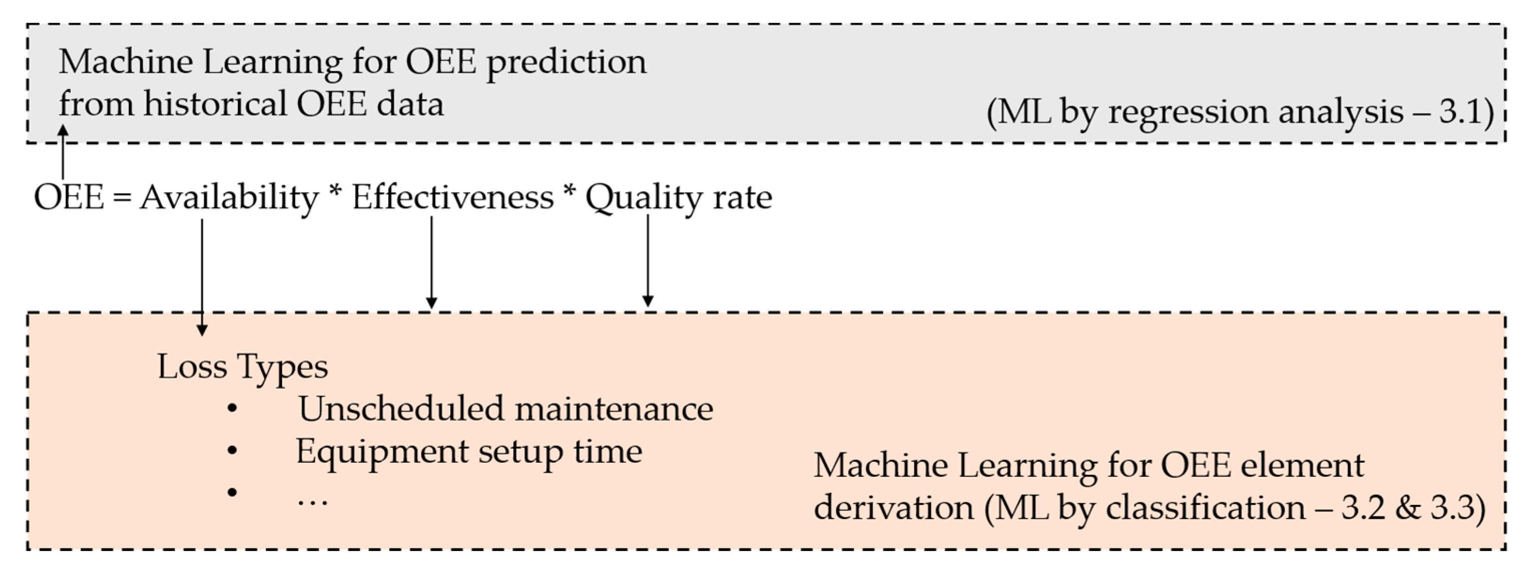Section 3 shows the main objective of the contribution. Here, the applicability of Machine Learning techniques to support the availability management by detecting changeover processes will be discussed (“data understanding” and “data preparation”). Furthermore, a use case is presented in order to illustrate the application of Machine Learning techniques identifying these changeover processes in a real production scenario (“data modelling”). The use case will focus on a detection of the start and stop point of the quick changeover process with Machine Learning. In Section 4, the results of the Machine Learning use case are discussed (“data evaluation”). In Section 5, the article will be summarized and an outlook to the upcoming research activities is given.

2. Availability Management

Machine availability has a strong influence on production planning and control. This is also evident in the study conducted by Schuh et al. in [4], in which the most frequent causes for deviations from the current production plan were surveyed from 89 study participants from the manufacturing industry in Germany: together with the acceptance of rush orders (63%), equipment failures, and malfunctions (56%) were the main causes for deviations followed by material shortages (39%) and the absence of personnel due to illness (34%)—multiple answers were possible.

To improve production planning and control, availability management must be established. It can be understood as the entirety of all activities and processes for achieving and maintaining demand-oriented availability of the production system, when considering organizational and technical factors [11]. There are already several strategies and concepts that pursue the goal of increasing and maintaining the availability of plants. The TPM concept has established itself in the field of maintenance organization in industry [12]. The concept was developed by Nakajima (1988) and adapted to the needs of Western companies by Hartmann (1992) [13,14]. For the calculation of availability in the machining production, the VDI guideline 3423 can also be applied [15]. Although VDI 3423 does not take into account the actually produced quantity per time unit into account [16], both of the approaches are standardized by ISO and the Association of German Engineers (VDI), which is of importance for the OBerA partners to guarantee comparability and robustness.

2.1. Availability According to TPM

A core element of TPM as an approach for a maintenance organization is the Overall Equipment Effectiveness (OEE), which is a metric for identifying the production losses of a machine or production facility [17]. The OEE indicator is divided into three sub-indicators: availability, performance, and quality. It represents the unused optimization potential and losses of a machine or production facility [18]. To increase the OEE indicator, the TPM aims at eliminating the six sources of losses according to Hansen in [19]:

• plant failure due to technical and organizational disturbances,
• losses due to setup and changeover,
• losses due to idle running and short shutdowns,
• losses due to reduced cycle speed,
• quality deviations, and
• start-up losses.

These system losses cause both time and volume losses, which can be divided into the factors performance, quality, and availability. ISO 22400-2 [20] defines OEE as the product of availability, effectiveness, and quality rate:

$$OEE=Availability · Effectiveness · Quality rate$$

(1)

The availability is calculated as the relation of actual production time (APT) to planned busy time (PBT). It also shows the plant capacity used for production in relation to the available plant capacity.

$$Availability= \frac{APT}{PBT}$$

(2)

The effectiveness represents the relationship between the optimal cycle time and current cycle time as planned runtime per item (PRI) multiplied by the produced quantity (PQ) divided by APT. The effectiveness shows how effectively a production system works during the production time.

$$Effectiveness= \frac{PRI·PQ}{APT}$$

(3)

The quality rate indicates the ratio between the quantity of good parts produced (GQ) and PQ.

$$Quality Rate= \frac{GQ}{PQ}$$

(4)

Table 3. Overall Equipment Effectiveness (OEE) factors combined with six loss types and possible causes of loss [21,23].

OEE Factor	Loss Type	Cause of Loss
Availability	Equipment failure	Device failure Main component failure Unscheduled maintenance
	Setup and adjustment	Equipment setup time Raw material shortage Lack of workforce
Effectiveness	Idling and minor stoppages	Short-time device failure (<5 min) Dropped product Blocking obstacle
	Reduced speed	Device not at nominal speed Untrained operator Idle state
Quality rate	Quality deviations in the production process	Scrap Rework Damaged in the process
	Deviations from product changeover	Scrap Rework Damaged in the process

shows how the three OEE factors can be combined with the six sources of loss, as mentioned above. The corresponding causes of loss in the table below support the data selection process for the calculation of the components of OEE calculation. For the successful calculation of OEE, the ability to collect data is of utmost importance, as if data is unreliable, the calculated OEE value does not reflect the utilization of the production unit [21]. Therefore, the quality of the data determines the accuracy of OEE. For this reason, the plant must first be analyzed, an ideal condition defined, and a possible cause/fault catalog determined. Subsequently, the causes must be evaluated according to their failure effect e.g., by means of a Pareto diagram and appropriate measures must be taken.

At the beginning of establishing the OEE metric, a production facility usually has an OEE between 30% and 60%, whereas companies in the automotive industry reach peak values of over 85%. OEE depends on the type production facility. A single machine has a higher OEE value than an interlinked production chain [22].

2.2. Availability According to VDI Guideline 3423

Another possibility for calculating an availability of single machines or production systems is the VDI guideline 3423. This guideline serves as a basis for contract negotiations between machine manufacturers and end users, as well as for internal optimization of production environments. The calculation of the availability of technical equipment according to VDI guideline 3423 is based on a past-oriented period calculation [24].

The technical availability is defined in the following way:

$$V_T=\frac{T_N}{T_B-T_O}=\frac{T_B-\left(T_O+T_T+T_W\right)}{T_B-T_O}$$

(5)

Additionally, the total utilization ratio is defined:

$$N_G=\frac{T_N}{T_B}=\frac{T_B-\left(T_O+T_T+T_W\right)}{T_B} · 100\%$$

(6)

Table 4. Variables for availability calculation according to VDI 3423.

Variable	Description
Organizational downtime TO	It is caused by shortcomings in the organization, e.g., energy shortfall, lack of workpieces or tools or training, a short-term lack of jobs, changeover time
Technical downtime TT	It is the sum of all downtimes which are caused by the design/construction of the machine manufacturer
Test time TC	The machine is used for testing purposes
Preventive maintenance time TW	Time which is used for scheduled maintenance
Utilization time TN	Time when the machine works at full capacity
Occupied time TB	Time for which any utilization of the machine is planned

shows the variables used in the above equations.

2.3. Comparison of TPM OEE and Availability According to VDI 3423

Both presented approaches of TPM OEE and availability according to VDI 3423 have in common that they relate the current production situation, which is influenced by losses (OEE) or downtimes (VDI 3423) to a planned situation. In particular, the calculation of availability according to VDI 3423 and availability according to the OEE indicator differ in the following aspects:

• When calculating the availability according to the OEE indicator, planned downtimes are not included, whereas the VDI guideline allocates planned work according to the maintenance plan (inspection, maintenance, cleaning) to the occupied time. The availability factor of the OEE is higher than the availability level when compared to the VDI guideline due to the non-inclusion of the planned preventive maintenance measures. The TPM concept supports preventive maintenance measures, but, if they were considered, they would have a negative impact on the OEE ratio. From a different perspective, it can be concluded that shortening the duration of preventive maintenance measures does not have a positive effect on availability [11].
• OEE combines organizational with technical downtimes. This is not the case in the VDI guideline.
• The VDI guideline also describes the test time during which a system is used for testing. If a production progress is generated by the test, this is assigned to the usage time, otherwise it is to be added to the organizational downtime (DIN 13306:2018-02). The calculation basis OEE does not mention test times. Tests are always planned in advance. For this reason, they are assigned to the planned downtime. As a result, the test time is not included in the calculation of OEE.
• VDI 3423 does not define how to deal with breaks or shift change. The utilization time considers a machine in order to produce at full capacity. Therefore, these time-shares are considered as downtimes, as production could have been done during the break. This is intended to create incentives to keep the system running by rotating the employees. According to the availability factor of the OEE, these are also not included in the calculation.
• As described, production is carried out at full capacity during the utilization time. VDI 3423 does not explicitly consider the effectiveness losses when compared to OEE. However, a distinction would be useful for internal operational improvement to identify performance deficits [18].
• Setup times are only considered as availability loss in the availability calculation according to OEE if the setup time default values are exceeded, whereas, according to the VDI guideline 3423, they are completely considered in the organizational downtime.
• The OEE uses the actual production time as the basis for the calculation of the availability. The VDI guideline does not use the actual production time, but uses the occupied time.
• The VDI guideline 3423 ignores the effectiveness and quality losses, although these are helpful for evaluate production performance. These are mentioned in the guideline by notes, but are not included for reasons of operational relevance, as they are strongly product related.

From the comparison above, it can be concluded that the two calculation approaches have different focus points, which results in a different assignment of losses/downtime to calculation elements. To illustrate the outcome of the different calculations, a scenario calculation was carried out with the same input data or each approach to show the effects of the different calculations of OEE and VDI 3423. The underlying data were taken from a consortium partner of the OBerA project.

Table 5. Comparison of an availability calculation from a production facility of an OBerA consortium.

Availability Calculation Approach	One Shift Basis [%]	Two Shift Basis [%]
VDI 3423	46.43	42.78
OEE	60.29	54.48

shows the results. Depending upon the calculation approach, different availability values arise. The availability according to OEE is higher compared to the VDI 3423 guideline showing a difference of over 10%. This can be attributed to the short downtimes, which are not included in the availability calculation for OEE.

2.4. Conclusion on Availability Management in Terms of Machine Learning

The previous chapter has shown that, depending on the calculation metric, different numerical results for an availability indicator can occur. Accordingly, before an availability can be forecasted or dedicated, OEE elements are to be calculated by means of Machine Learning, the particular metric needs to be selected and each element of the metric needs to be defined and traced back to available data sources in the related company. It must be clarified where and how this data can be obtained.

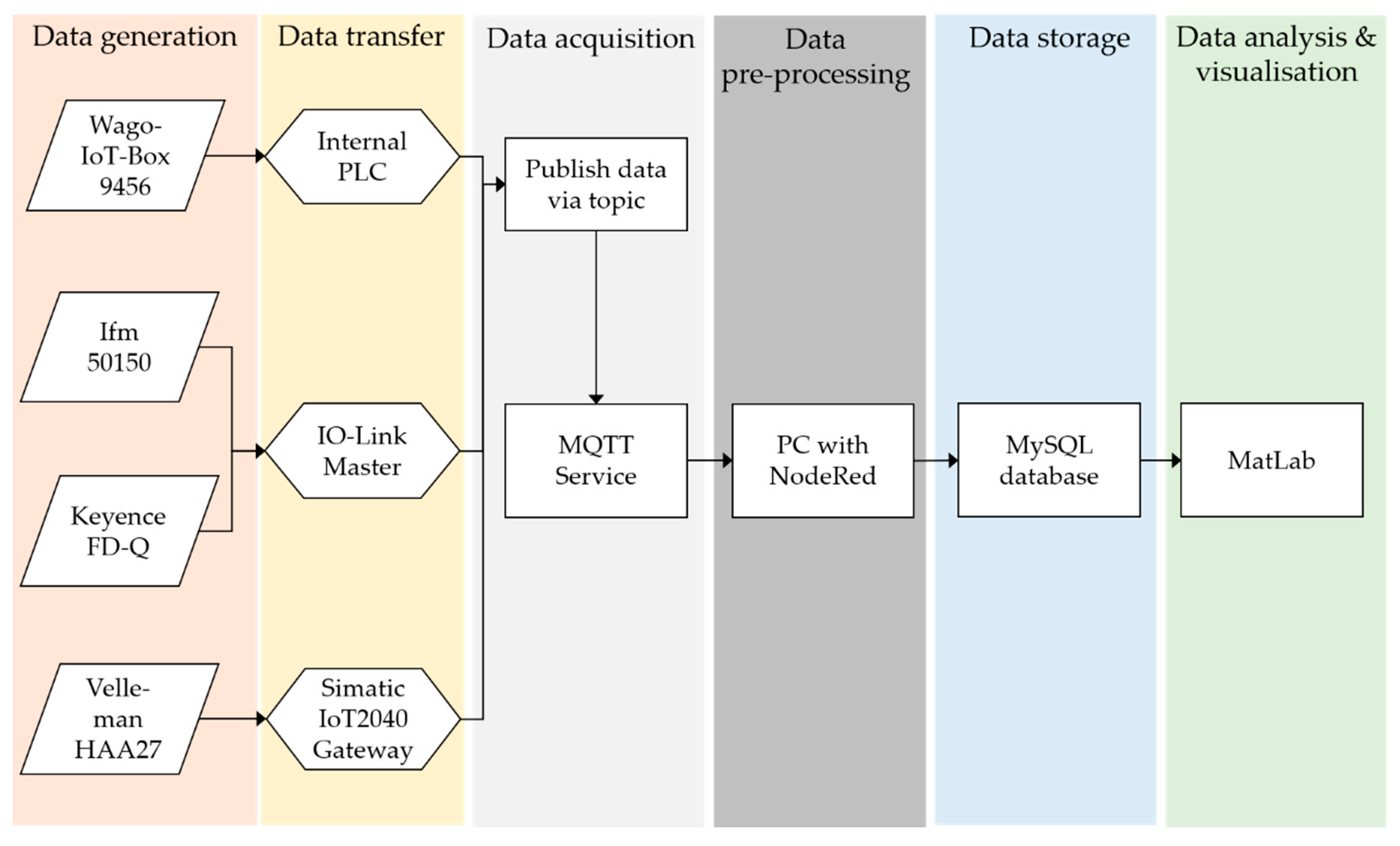
The elements needed to calculate OEE and its components, plant availability, effectiveness and quality, are defined in ISO22400-2 [20]. The standard divides these elements additionally into the subcategories time elements, logistics elements and quality elements. The planned busy time and the planned running time per item can be assigned to the planned times and the actual production time to the actual times. The quantity produced and the quantity of good parts produced are classified as logistics elements. While the plannable time elements can be read from the ERP system, the actual times that are required must be measured directly at the machines or lines. In CPPS, this is done via sensors that record machine and product statuses and store the read-out sensor data in databases or pass them directly to a Manufacturing Execution System (MES) [25].

Table 6. Elements of OEE calculation (ISO 22400-2, Hwang 2017).

OEE Element	ISO 22400-2 Category	Data Source (Hwang 2017)
planned busy time (PBT)	Planned time	ERP
planned runtime per item (PRI)	Planned time	ERP
actual production time (APT)	Actual time	Sensor
produced quantity (PQ)	Logistic element	Sensor
quantity of good parts produced (GQ)	Logistic element	Sensor

shows the data sources where OEE elements can be retrieved from. For the planned elements of the calculation, Hwang [26] locates the Enterprise Resource Planning System (ERP-system) as the data source. Current production information is generally retrieved from sensors.

This is also applicable for the VDI 3423.

Table 7. Elements of VDI 3423 calculation.

VDI 3423 Element	Category	Data Source
Organizational downtime TO	Actual time	Sensor
Technical downtime TT	Actual time	Sensor
Preventive maintenance time TW	Planned time	ERP
Utilization time TN	Actual time	Sensor
Occupied time TB	Planned time	ERP

shows how the main elements can be categorized correspondingly:

The experience from the research project OBerA is that, apart from these theoretical considerations above, the practical situation in SME companies is more complex than to distinguish between ERP and sensors as data sources:

Sensors often are realized manually and not necessarily as CPPS sensor networks in SMEs. Examples range from manual input into computer terminals on the shopfloor, tally sheets with manual transfer into Microsoft Excel, to manually triggered signals in programs of machine controls.

ERP-systems in SMEs can range from fully fledged ERP installations with sub modules for maintenance management and manufacturing execution (MES: manufacturing execution system) to heterogeneous software platforms for individual purposes and production data terminals for manual feedback of manufacturing order statuses.

Table 8. IT system landscape of the OBerA partners.

Company	ERP System	Production Planning System	Tool Management System	Shopfloor Data Collection System
Brehm	Pro Alpha	Pro Alpha	Tally sheet	-
Franken	SAP	SAP	SAP based	-
Kritzner	Braininfor	FELIOS	TDM	-
Pabst	ERP Bios2000	ProMExs	-	GeoVision, GNT-Systems
Siemens	SAP	Preactor APS	Self-programmed	AMP

illustrates this situation by giving an overview of the different IT systems which are used in the consortium as ERP system, production planning system, tool management system, and shopfloor data collection system.

The situation is also aggravated by the current development that MES can serve as sensor connection platform, which is synchronized with the ERP, offering the possibility that the MES also directly calculates the indicators as OEE. The MES can serve as an intermittent layer between classical sensors and the ERP. The OEE calculation approach of the MES often remains not transparent.

In conclusion, it must be stated that there are no simple recipes to find data sources for the OEE elements of the calculations. Moreover, a data source plan must be developed with a project team consisting of experts from the machine manufacturers, machine control manufacturers, the enterprise software manufacturers, maintenance, and quality management staff, who have a common and clear understanding of the calculation components and the systems, which deliver the necessary data. A contribution to derive OEE elements or predict the OEE from sensor data is Machine Learning as a part of Cyber Physical Production Systems.

3. Machine Learning in the OEE Context

Based on the discussion regarding the different concepts of availability and OEE indicator calculation ML can contribute to transform traditional mechatronic production systems in CPPS as customizable data collection systems [27]. In this context, two approaches are presented in the following. First, ML for OEE prediction is reviewed in Section 3.1. And, second, the suitability of ML for identifying changeover processes as an OEE element is shown in Section 3.2. Section 3.3 presents the latter concept in detail and its application in a real production scenario. Figure 1 illustrates the different ML approaches that are discussed in this chapter.

3.1. Machine Learning Application for OEE Prediction

In the following, four studies are reviewed that use ML algorithms to calculate or predict the OEE, the predictive OEE (POEE), as a variation of OEE or the plant availability (AE), as well as OEE elements.

Table 9. Studies on Machine Learning for OEE prediction.

Authors (Year)	KPI	Investigated ML Algorithms	Prediction	Failure Mode Analysis	Data Quality Analysis	Basis: Sensor Data	Multiple Machines	Best Prediction
El Hassani et al. [28]	OEE	SVN, RF, EGB, DNN	●	◯	●	./.	◯	DNN, RF
Liao et al. [29]	POEE	LSTM, DQN	●	◯	./.	●	◯	LSTM
Kuo & Lin [30]	AE	DNN, DT	●	◯	./.	./.	◯	DNN, DT
Ecker & Hellfeier [31]	OEE	./.	●	◯	./.	●	●	./.

includes the author and year of publication of the study, the KPI considered, and the ML algorithms used for the calculation. In addition, relevant criteria are named for this research. This allows for a critical comparison of the studies. These criteria are the part of the OEE calculation, prediction and failure cause analysis, the basis of calculation for sensor data or the number of machines as well as the data quality. Criteria listed in the studies were marked in the Table 9 by a “●”, untreated factors by a “O”. In the fields that are marked with a “./.”, the considered studies do not focus on this aspect. Finally, the ML algorithms that scored the best in the studies were mentioned in the last column.

El Hassani et al. [28] use various ML algorithms to predict the OEE of a cable manufacturer. For the calculations, the authors use Support Vector Machines (SVM), Random Forests (RF), Extreme Gradient Boosting (EGB), and Deep Neural Networks (DNN). El Hassani et al. use a model based on ML algorithms to predict the OEE of a machine and, thus, provide managers with a decision-making tool. With the help of these calculations, managers can derive measures to prevent the loss, even before it occurs and, thus, keep the performance of the machine at a high level. The research group concludes that DNN and RF with cross-validation can most reliably predict OEE.

Kao et al. [32] describe in a study the Predictive Overall Equipment Efficiency (POEE) as a KPI for predicting OEE. In this study, predictions are made for all three sub-KPIs of OEE. The study refers to a single machine for chemical vapour deposition in the semiconductor industry. Through the POEE, appropriate measures can be taken in order to prevent losses in machine performance. Liao et al. [29] forecast the predictable elements with different neural networks that are based on these POEE. A combination of Long Short-Term Memory (LSTM) and Reinforced Deep Q-Networks (DQN) is used. The preliminary results show that the predictions of the ML model are more robust against noise in the data as compared to classical models. Such benefits could result from using the long-term memory function of the LSTM in the Machine Learning model.

Kuo and Lin [30] calculate the plant availability of a TFT-LCD washing machine with different neural networks and decision trees. By calculating the plant availability as part of the OEE, a first step towards the prediction of the overall OEE is made. The calculation is performed by combining different neural networks of the type Back Error Propagation (BEP) and decision trees (DT) with the C5.0 algorithm. In total, four different models are used. The first uses a pure neural network, the second a neural network with specially adapted nodes, the third model uses a neural network in combination with a decision tree and, the fourth, a neural network with special nodes in combination with a decision tree. Kuo and Lin [30] conclude that methods 1, 2, and 3 have similar accuracy and perform better than method 4. Methods 1 and 2 show little variation: the predicted values do not provide useful information for managers. The predicted values of method 3, the combination of a neural network and a decision tree, are the most likely to represent reality. Method 3 can accurately predict a downward trend in the period under consideration in three weeks and approximately in four weeks. Ecker and Hellfeier [31] develop another model for calculating OEE with ML algorithms. The authors try to improve the OEE of a production plant in massive forming by predictive maintenance. For this purpose, they use the software Genius CM, which first records process data and sensor signals of a plant and incorporates them into the analysis of the OEE. In this way, the authors strive to display process-dependent conditions well and record dependencies between production parameters and system status. The presented model has not yet been applied to a data set for calculation, so there is no information on the algorithms used.

The previous brief review of ML approaches to predict OEE leads to the question how ML can also contribute to derive elements of OEE e.g., changeover times, as CPPS are equipped with numerous sensors. In this context, Yoon et al. [33] point out that the mathematical models used in smart factories should be able to process information in real-time, which they believe is crucial to be able to react quickly to changes in the process. Further, the research group of Yoon et al. stated that it is even more important to consider the inter-process relationships of an entire production line [31]. The processing of real-time information involves the collection, analysis, and application of information that is derived from data. Despite the new possibilities of the Internet of Things (IoT) and CPPS, they see the collection of data in the process lines as a major problem, as it is difficult to collect and process the data in real-time [31].

Chabowski et al. identify the availability as a major contributing element for OEE (around 85%, as compared to 99.92% effectiveness and 99.72% quality rate) [34]. The research group detected it through a cause and effect analysis. Changeover activities are the main reason (37%) for decreasing OEE, followed by technical breaks (~28%). Additionally, Vega et al. [35] address the importance of changeover and develop a model to indicate and operationalize changeover processes, which implies that the changeover times have to be shorter and reduce the costs associated with them to be competitive. These processes accumulate and add no value to the product, especially in flexible SME companies, which tend to produce in small lot sizes.

3.2. Suitability of Machine Learning for Quick Changeover

Setup, or changeover, time includes the total time that is required to prepare a work system for the completion of tasks (changeover), as well as to restore it to its original state [36].

In traditional, non-CPPS based factories, the “Single Minute Exchange of Die” (SMED) method is used in order to minimize changeover time and well known in Lean Management [37]. Positive effects of quick set-up include increased equipment utilization (OEE) and improved transparency in planning and production. SMED is mostly done offline in Lean Management workshop formats without considering sensor data. Further consequences of minimizing setup times include the reduction of inventories and unit costs [38]. At the beginning of the SMED process, the changeover process to be optimized is selected and then its current workflows are documented with the help of spaghetti diagrams or reports. Subsequently, a distinction is made between the external internal changeover processes and it is checked whether certain internal changeover processes can be dispensed with or whether they can be converted into external changeover processes. The focus here is on optimizing the internal changeover processes in order to reduce downtimes. External changeover processes can be shortened, for example, by parallel changeover and the elimination of time-consuming adjustments. Finally, the production environment can be improved by coordinating the sequence of changeover processes and optimizing the deployment of personnel.

The successful implementation of CPPS solutions requires efficient data integration in order to realize the same optimization than the SMED method. For example, it is necessary to interpret the machine signals to evaluate the operating states of the machine [39]. In the context of production optimization, these machine signals are used, among other factors, in order to determine the overall equipment effectiveness (OEE). This involves integrating the data from a normally functioning plant into a data model to train it and identify limit values or existing data pattern. If anomalies are detected in future data sets, this can indicate, for example, that the system is malfunctioning [39,40].

The necessary data are collected from information sources, such as sensors, and the corresponding machine telemetry, pre-processed, and essential features are extracted. Furthermore, condition monitoring enables the determination of the reason for a machine failure. Anomalies and events can be identified by means of classification techniques such as decision trees [41]. Predictive maintenance extends condition monitoring by forecasting models, which allow for example trend analyses and the calculation of the remaining plant utilization period. Forecast models can be used to predict when the next fault is expected and proactively trigger a machine event to prevent it.

Human-machine interfaces are increasingly important due to the increasing complexity of production plants [40]. Likewise, the achievement of small batch sizes is a decisive competitive factor, so the reduction of set-up times is of great importance [42]. However, it is not feasible to derive waiting times, for example, for workpiece loading, purely from machine signals and, therefore, requires information from higher-level systems [39]. Furthermore, an interpretation of the downtime between job start and production signal cannot be assumed as a setup time by the machine. Only by integrating job information and manually entered information a setup can phase be interpreted for the data model [39]. Hence, ML can be a feasible approach for distinguishing changeover and production phases by a model that was trained by datasets from machine sensors.

3.3. Application of ML in Changeover Processes

3.3.1. Use Case Description

The company Pabst GmbH is a medium-sized family business that is split into two sections: Automotive and Component Production. The section automotive provides serial production, aftermarket, and prototypes. All of the sections are characterized by small lot sizes of 10–200 workpieces. The component production contributes to spindle-/drive-technology, mechanical engineering, and aerospace. For this contribution, a CNC milling machine from the component production is used to apply ML for OEE element derivation. The very low accessibility of machine data and, in consequence, limited insight into crucial information that could be used to improve set-up and production time, leads to a retrofit with five sensors, which are listed in

Table 10. All of the sensors used to generate machine data.

Sensor Type	Measuring Object	Measuring Type
Ifm 5D150	Door status tool holder	Distance measurement
Keyence FD-Q Series	Coolant flow	Flow measurement
Velleman HAA27	Door status workpiece holder	Contact measurement
Velleman HAA27	Door status machine main door	Contact measurement
Wago IoT-Box 9466	Machine power/performance	Power measurement

.

The Ifm 5D150 is a distance sensor that measures the distance from its mounting point to the handle of the tool holder. If the tool holder is being opened, then the distance decreases and the sensor sends the signal that the door is open and vice versa. The Keyence FD-Q Series measures the coolant flow of the machine. As soon as the machine starts pumping the coolant, the sensor recognizes the flow. Both Velleman HAA27 sensors are used in order to monitor the workpiece and machine main door individually. Each sensor consists of two magnet switches, which generate a digital signal if they come close enough to each other. With a Wago IoT-Box 9466 the power of the machine is measured by Rogowski coils. The sensor concept, as well as the retrofitted milling machine, is illustrated in Figure 2. The goal is to generate, combine, and evaluate the data from all of the sensors to predict machine behavior. The motivation of Pabst GmbH management is to generate a link between customer order and necessary setup-time to fulfill it. The setup-time adds no value to the products and should be minimized in terms of increasing the OEE. Additionally, different workers, who perform different procedures to changeover a machine, perform the setup-process. This instance influences the sensor data induced pattern of the entire changeover process, which should be identified by the ML model.

3.3.2. Data Handling Concept and Data Preparation for Machine Learning

Additional equipment is needed in order to acquire the data from the five installed sensors at the machine. An LTE-Router and an Ethernet switch provide internet access to all sensors via LAN. Both the Ifm 5D150 and Keyence FD-Q Series are connected to an IO-Link master, which controls the communication with all connected IO-Link devices. The Velleman HAA27 contact switches are attached to the Simatic IoT2040 gateway. The gateway reads the digital signals generated by the contact switches. The Wago IoT-Box has a built in PLC and can send data using different methods. All mentioned devices are capable of transmitting data messages through the MQTT protocol. At last, a PC is necessary to subscribe to the different data message topics of each sensor. For this case, an Intel-NUC-Mini-PC is used, with the application Node-Red installed. Node-Red is a platform for integrating IoT equipment in combination with a graphical programming language. It provides a convenient way to subscribe to the different data message topics and to transform the data into a usable format. Finally, all of the data are stored into a SQL database. The data from all sensors are generated in rows and columns, displaying the ID, timestamp, topic, value, measure, and sensor name. For the ML classification problem, each data set is labelled with “changeover” or “production”.

Table 11. Database excerpt.

ID	Datetime	Coolant Flow [l/min]	Door 1	Door 2	Door 3	Power [Watt]	Status/Label
…	…	…	…	…	…	…	…
10000	21.07.2020 08:15:00	33	1	1	1	3370.68	Changeover
10001	21.07.2020 8:15:01	33	0	0	1	3375.98	Changeover
…	…	…	…	…	…	…	…

shows the data structure of each set.

Rautmare and Bhalerao [43] compared the performance of a traditional MySQL database to the NoSQL database MongoDB for IoT applications. They tested both database types by steadily increasing the amount of data and load on the system. Even though MongoDB required less response time than MySQL, the latter had more stable response times. Concluding, the authors in [43] state that choosing the right database depends on the use case. Phan et al. [44] performed a similar study, comparing different MySQL and NoSQL databases for IoT. They came to the same conclusion—that every database has its pros and cons. Therefore, MySQL is chosen over other databases to store the generated data. In summary, Figure 3 shows the complete process from data generation to data analysis.

The generated data are processed with a Node-Red flow and then exported to a MySQL database. To minimize data traffic, only decisive values are transmitted and stored [45]. For this reason, the sampling rate per sensor was set to 1000 ms.

The detection and handling of missing or incorrect data, as well as their uniform presentation, are the main objectives of the data pre-processing step [46]. A prerequisite for the processing of sensor data is the coupling of the sensor technology with a communication standard, such as MQTT [45]. With the help of MySQL Workbench, the observation period is limited and the data are extracted in the form of a.csv file. To enable the application of the algorithms in the following steps, the acquired data are adapted to the form of an “analytics base table” (ABT). An ABT corresponds to a basic tabular structure according to which historical data sets can be built up for analytical evaluation [47]. The column headings of the table include several descriptive characteristics and a target variable. Each row corresponds to an instance for which a prediction can be made and is filled with values for the descriptive characteristics and the target variable [47]. The target variable corresponds to the setup progress, which is determined depending on the sensor data (descriptive characteristics).

The processing of the data in terms of outliers, trends, totals, minima, maxima, and averages is important [48]. Outliers in the data set can be classified if they differ from the mean value by at least twice of the standard deviation [46]. The definition of a permissible value range is applied to exclude the possibility that data points are incorrectly classified as outliers [46]. The detected outliers can, for example, be replaced by mean values of the data. Filter methods are particularly suitable for the detection and correction of outliers in time series [46]. Suitable filter methods include exponential, discrete, and linear filters. Whether data are sufficient for a Machine Learning based model or not becomes clear when patterns are detected. Hence, it is not possible to predict which data are required for model quality and accuracy.

As cloud platforms, e.g., Microsoft Azure for ML, are barely used in SMEs applications [49], the ML model is implemented in the MatLab environment. Machine learning algorithms show significant variability within different problems and metrics in terms of their accuracy [50]. By utilizing the Matlab “Classification Learner”, various available algorithms are applied to the specified changeover detection problem above and then the accuracies of the trained models are compared. For the study data of one-day series production with a sample rate of 1000 ms was collected. 36.844 datasets were recorded and have been labelled accordingly (changeover, production). 4176 datasets with changeover status and 32.668 for production were detected. The next paragraph shows the results of the study.

3.3.3. Machine Learning Results

Several ML-techniques were evaluated with the Matlab “Classification Learner” that might fit the described use case as a classification problem. The methods evaluated show different performance level. Decision Trees and Ensemble Classifiers show good results for the underlying problem. Decision trees are characterized by a high prediction speed, low memory usage, and easy interpretability. These classifiers are a top down approach beginning from a start condition. The tree brakes down until reaching the leaf nodes by checking decision nodes. The authors also state, that Ensemble Classifiers combine the power of individual classifier, as distributed training data are run repeatedly on weak learners and combined into a strong classifier with high accuracy [51]. The evaluation with the mentioned data set from the use case shows that “Fine Tree”, as a type of Decision Tree algorithm, proved to be the most fitting with an overall accuracy of 92.8% (see Figure 4).

Although the “Fine Tree” algorithm has the highest overall accuracy, difficulties appear in the recognition of the “Changeover” class. The confusion matrix shows the true/false positive rates. Here, it can be seen that, especially, the classification of the changeover datasets are critical (Figure 5 left). When analyzing the confusion matrices of all tested algorithms, the RUSBoosted tree as a type of an Ensemble Classifier showed the highest accuracy in the recognition of the class “Changeover” (Figure 5 right). Despite a lower accuracy, the confusion matrix of the RUSBoosted tree show a significantly improved true/false positive rates.

The ROC Curves of Fine Tree and RUS Boosted Tree are also compared (see Figure 6) through the tradeoff of the true and false positive rates to investigate the model quality on various probability levels from 0 to 1. The quality of the classifier is then quantified by the area under curve (AUC). Here, the RUS Boosted Tree shows a better result with 0.93 to 0.92 for the Fine Tree. Accordingly, despite that the overall accuracy of the Fine Tree is obviously higher, the classification of the changeover process can be done better with the RUS Boosted Tree algorithm.

Multiple Decisions Trees are combined, as the RUS Boosted Tree is an Ensemble Classifier. Figure 7 exemplarily illustrates one out of 30 trees. It can be seen that, after the starting condition of an opened/closed door, the sensors for coolant flow and power measurement determine the classification of “production” and “changeover”.

4. Discussion

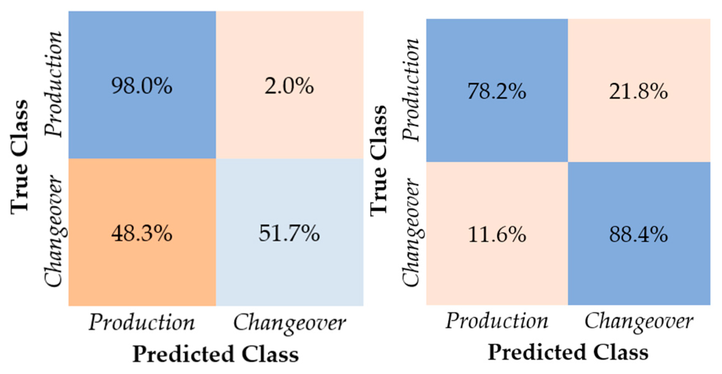
The results of the trained ML model show that it is possible to distinguish “production” and “changeover” phases on a reliable level in a serial production that is based on the presented sensor concept and data preparation method. Nevertheless, changeover processes are very heterogeneous in terms of their technical appearance and manual, worker related procedures, but they have an impact to the OEE and hence to the economic perspective of a company. The presented innovative approach of ML for classifying changeover automatically in the context of CPPS lead to a broader more adaptive functionality of machines, as technical and worker actions are both represented in the datasets. Generally, in CPPS, there is an increased interconnection of production machines. As a result, increasing data from the machines and processes are being collected automatically with the help of sensors. Due to the mass, speed and heterogeneity of the collected data, the industry is increasingly experiencing problems in evaluating this data, for example, in order to determine the performance of the processes precisely, traditional methods and analytical models have reached their limitations in this respect. Data-driven methods that use ML by a means of evaluating the data could be the solution here.

5. Conclusions and Further Research

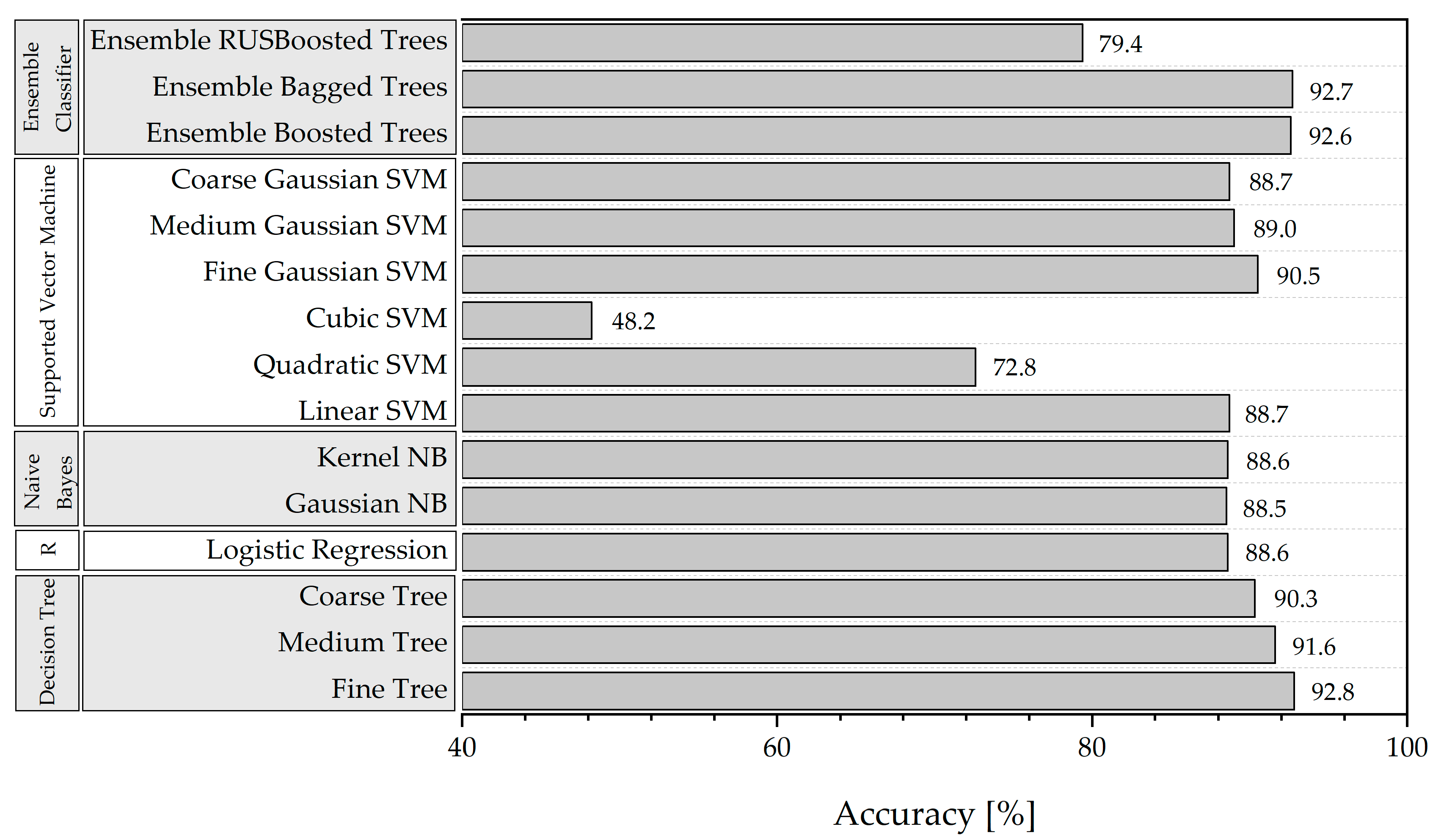
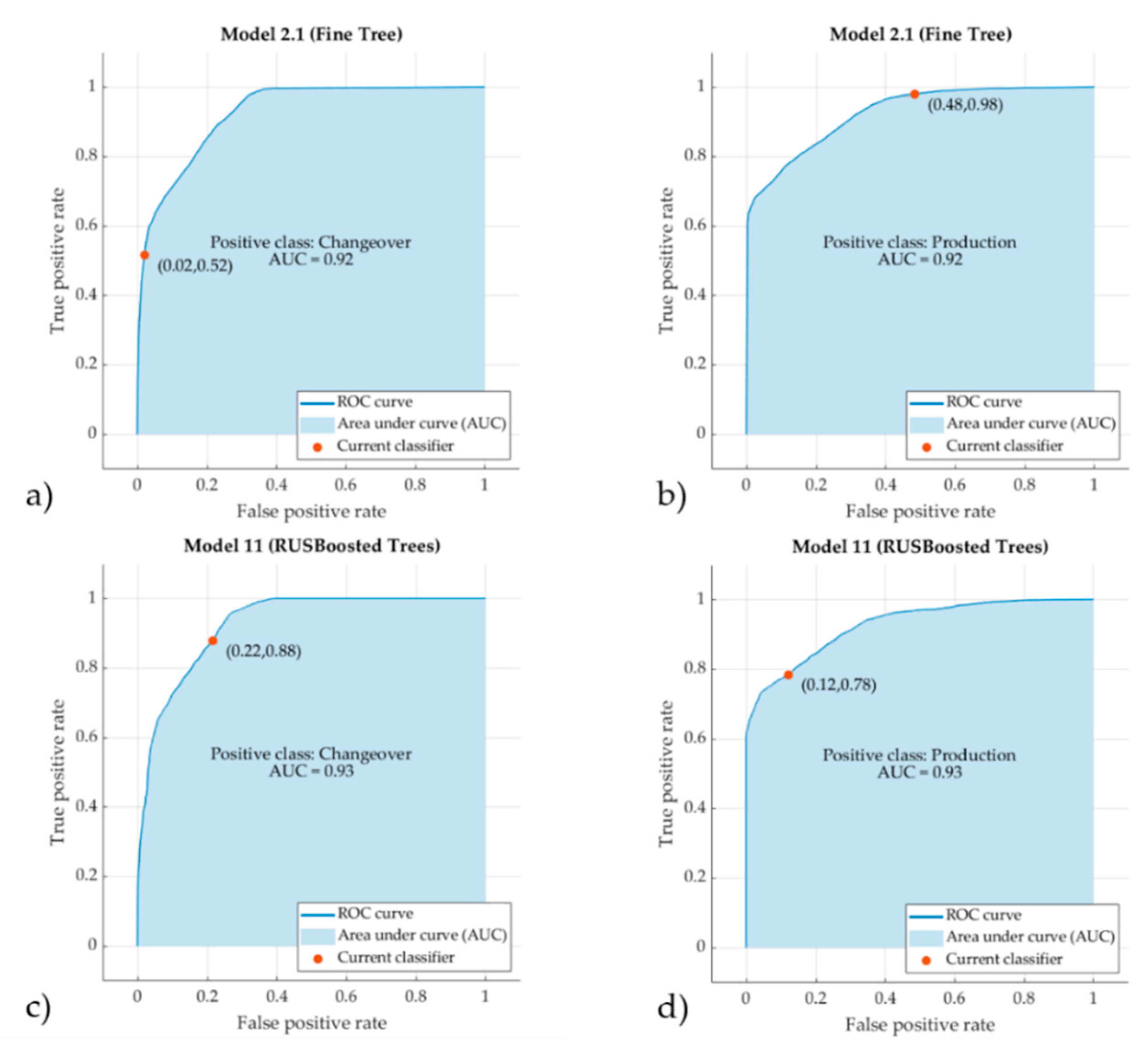
The contribution gives, at first, a theoretical insight into the different standards of availability management and shows the difference of the OEE and VDI 3423 approach. Within this analysis, the elements of both indicators become obvious. Here, the setup or changeover time is a crucial factor of OEE, which needs to be controlled. Furthermore, ML techniques might be suitable for the prediction of the OEE from historical data and the one hand. The paper reviews the state of research in this context. On the other hand, ML can contribute to distinguish changeover and serial production processes by a trained model to determine changeover times as an element of the OEE. This approach is presented more in detail. Thus, a use case scenario in a real production environment of the SME Pabst GmbH is shown. At this, the sensor concept and the data handling procedure is discussed before a huge data set is used in order to train several ML algorithms. The most promising Fine Tree and RUS Boosted Tree are investigated then in detail to find the best solution for the indicated classification problem. Recently, the ML changeover identification is used several times in the Pabst GmbH production for various products to validate the model again and gain more data for enhancing the ML approach.

Further research will be done in refining the classification in between the changeover as well as the production phase. This leads to a more complex multi-classification problem. The opportunity of this enhanced method is that, within production, idle phases of the machine can probably be identified as well as setup-subphases to predict the setup length. Both information can facilitate management decisions in terms of production planning and control. As a vision, the presented approach should automatically distinguish non-value-adding phases and recognize (time-)efficient changeover patters e.g., of different workers, which then serve as recommendations for other employees for their individual setup procedures. This can lead to self-optimizing production systems. Another research topic is the integration of ML methods into a general machine model in order to derive the OEE from heterogeneous data sources with the help of ML models, analytical as well as low-level information such as counters. In this case, the aim is to relocate the OEE calculation from business process level to the shop-floor, where the real value creation takes place. Here, the inter-process control loops need to be short in order to further increase efficiency in manufacturing companies specially for highly flexible SMEs.

References

1. Statistisches Bundesamt—Umsatz der Deutschen Metallindustrie in den Jahren 2005 bis 2017. Available online: https://de.statista.com/statistik/daten/studie/237217/umfrage/um-satz-der-metallindustrie-in-deutschland/ (accessed on 12 July 2018).
2. Nyhuis, P.; Münzberg, B.; Kennemann, M. Configuration and regulation of PPC. Prod. Eng. 2009, 3, 287–294. [Google Scholar] [CrossRef]
3. Schuh, G.; Gottschalk, S.; Höhne, T. High Resolution Production Management. In Advances in Production Management Systems. Sustainable Production and Service Supply Chains; Prabhu, V., Taisch, M., Kiritsis, D., Eds.; Springer: Berlin, Germany, 2007; pp. 439–442. [Google Scholar]
4. Schuh, G.; Prote, J.; Luckert, M.; Schmidhuber, M. Potenzial von Echtzeitdaten für die Produktion, Ergebnisse einer Studie des Werkzeugmaschinenlabors WZL der RWTH Aachen. Wt Werkstattstech. 2018, 108, 198–203. [Google Scholar]
5. Heins, M.; Nyhuis, P.; Pachow-Frauenhofer, J. Zustandsbeschreibung von Produktionsanlagen. Methodik zur Abbildung einer nachhaltigen Verfügbarkeitsverbesserung. Wt Z. Ind. Fert. 2008, 98, 622–627. [Google Scholar]
6. Hering, N.S. Echtzeitfähig-Koordinierte Produktionsplanung in Supply-Chains der Verbrauchsgüterindustrie, 1st ed.; Apprimus-Verlag: Aachen, Germany, 2014. [Google Scholar]
7. Schuh, G.; Potente, T.; Wesch-Potente, C.; Weber, A.R.; Prote, J.P. Collaboration Mechanisms to Increase Productivity in the Context of Industrie 4.0. Procedia CIRP 2014, 19, 51–56. [Google Scholar] [CrossRef] [Green Version]
8. Ghafoorpoor Yazdi, P.; Azizi, A.; Hashemipour, M. A hybrid methodology for validation of optimization solutions effects on manufacturing sustainability with time study and simulation approach for SMEs. Sustainability 2019, 11, 1454. [Google Scholar] [CrossRef] [Green Version]
9. Ghafoorpoor Yazdi, P.; Azizi, A.; Hashemipour, M. An empirical investigation of the relationship between overall equipment efficiency (OEE) and manufacturing sustainability in industry 4.0 with time study approach. Sustainability 2018, 10, 3031. [Google Scholar] [CrossRef] [Green Version]
10. Wirth, R.; Hipp, J. CRISP-DM: Towards a standard process model for data mining. In Proceedings of the 4th International Conference on the Practical Applications of Knowledge Discovery and Data Mining, Manchester, UK, 11–13 April 2000; Springer: London, UK, 2000; pp. 29–39. [Google Scholar]
11. Franzkoch, B. Wertorientiertes Verfügbarkeitsmanagement, 1st ed.; Apprimus-Verlag: Aachen, Germany, 2010. [Google Scholar]
12. REFA Bundesverband e. V. OEE—Overall Equipment Effectiveness. Available online: https://refa.de/service/refa-lexikon/oee-overall-equipment-effectiveness (accessed on 13 October 2020).
13. Nakajima, S. Introduction to TPM: Total Productive Maintenance; Productivity Press: New York, NY, USA, 1988. [Google Scholar]
14. Hartmann, E. Successfully Installing TPM in a Non-Japanese Plant: Total Productive Maintenance; TPM Press: Pittsburgh, PA, USA, 1992. [Google Scholar]
15. Willeke, N.; Uhlmann, E. Quantifizierung von Einsatzgrenzen einer zentralen und dezentralen Steuerungsstruktur. In Simulation in Produktion und Logistik; Putz, M., Schlegel, A., Eds.; Wissenschaftliche Scripten: Auerbach, Germany, 2019; pp. 356–367. [Google Scholar]
16. Putz, M.; Langer, T. Determination of extended availability and productivity for assembly systems using existing data base. CIRP Ann. Manuf. Technol. 2012, 61, 17–20. [Google Scholar] [CrossRef]
17. Koch, A. OEE für das Produktionsteam. Das Vollständige OEE-Benutzerhandbuch—Oder Wie Sie Die Verborgene Maschine Entdecken, 3rd ed.; CETPM Publishing: Herrieden, Germany, 2016. [Google Scholar]
18. Focke, M.; Steinbeck, J. Steigerung der Anlagenproduktivität Durch OEE-Management. Definitionen, Vorgehen und Methoden—Von Manuell bis Industrie 4.0, 1st ed.; Springer Gabler: Wiesbaden, Germany, 2018. [Google Scholar]
19. Hansen, R.C. Overall Equipment Effectiveness. A Powerful Production/Maintenance Tool for Increased Profits, 1st ed.; Industrial Press: New York, NY, USA, 2001. [Google Scholar]
20. ISO 22400-2:2014. Automation Systems and Integration—Key Performance Indicators (KPIs) for Manufacturing Operations Management, Part 2: Definitions and Descriptions; International Standard Organization (ISO): Geneva, Switzerland, 2014. [Google Scholar]
21. Jeong, K.Y.; Phillips, D.T. Operational efficiency and effectiveness measurement. Int. J. Oper. Prod. Manag. 2001, 21, 1404–1416. [Google Scholar] [CrossRef]
22. Singh, R.; Shah, D.B.; Gohil, A.M.; Shah, M.H. Overall Equipment Effectiveness (OEE) calculation-Automation through hardware & software development. Procedia Eng. 2013, 51, 579–584. [Google Scholar]
23. Chandra, A.; Chaturvedi, Y.; Kumar, A. OEE enhancement using TPM in light machine shop: A case study. Int. J. Appl. Eng. Res. 2018, 13, 202–208. [Google Scholar]
24. Linß, G. Qualitätssicherung—Technische Zuverlässigkeit. Lehr- und Arbeitsbuch, 1st ed.; Carl Hanser Verlag GmbH Co KG: München, Germany, 2016. [Google Scholar]
25. Helu, M.; Libes, D.; Lubell, J.; Lyons, K.; Morris, K.C. Enabling smart manufacturing technologies for decision-making support. In Proceedings of the International Design Engineering Technical Conferences and Computers and Information in Engineering Conference, Charlotte, NC, USA, 21–24 August 2016. [Google Scholar]
26. Hwang, G.; Lee, J.; Park, J.; Chang, T.W. Developing performance measurement system for Internet of Things and smart factory environment. Int. J. Prod. Res. 2017, 55, 2590–2602. [Google Scholar] [CrossRef]
27. Pérez, F.; Irisarri, E.; Orive, D.; Marcos, M.; Estevez, E.A. CPPS Architecture approach for Industry 4.0. In Proceedings of the 2015 IEEE 20th Conference on Emerging Technologies & Factory Automation, Luxembourg, 8–11 September 2015; pp. 1–4. [Google Scholar]
28. El Hassani, I.; El Mazgualdi, C.; Masrour, T. Artificial Intelligence and Machine Learning to Predict and Improve Efficiency in Manufacturing Industry. Available online: https://ui.adsabs.harvard.edu/abs/2019arXiv190102256E (accessed on 10 May 2019).
29. Liao, D.Y.; Tsai, W.P.; Chen, H.T.; Ting, Y.P.; Chen, C.Y.; Chen, H.C.; Chang, S.C. Recurrent Reinforcement Learning for Predictive Overall Equipment Effectiveness. In Proceedings of the 2018 e-Manufacturing & Design Collaboration Symposium, Hsinchu, Taiwan, 7 September 2018; pp. 1–4. [Google Scholar]
30. Kuo, Y.; Lin, K.P. Using neural network and decision tree for machine reliability prediction. Int. J. Adv. Manuf. Technol. 2010, 50, 1243–1251. [Google Scholar] [CrossRef]
31. Ecker, M.; Hellfeier, M. Forecast Model for Optimization of the Massive Forming Machine OEE. In Asset Intelligence through Integration and Interoperability and Contemporary Vibration Engineering Technologies, Proceedings of the 12th World Congress on Engineering Asset Management and the 13th International Conference on Vibration Engineering and Technology of Machinery, Brisbane, Australia, 2–4 August 2017; Mathew, J., Lim, C., Ma, L., Sands, D., Cholette, M., Borghesani, P., Eds.; Springer: Cham, Germany, 2017; pp. 147–156. [Google Scholar]
32. Kao, Y.T.; Chang, S.C.; Dauzere-Peres, S.; Blue, J. Opportunity for improving fab effectiveness by predictive overall equipment effectiveness (POEE). In Proceedings of the 2016 e-Manufacturing and Design Collaboration Symposium 2016, Hsinchu, Taiwan, 9 September 2016; pp. 1–4. [Google Scholar]
33. Yoon, S.; Um, J.; Suh, S.H.; Stroud, I.; Yoon, J.S. Smart Factory Information Service Bus (SIBUS) for manufacturing application: Requirement, architecture and implementation. J. Intell. Manuf. 2019, 30, 363–382. [Google Scholar] [CrossRef]
34. Chabowski, P.; Rewers, P.; Trojanowska, J. Impact of shortening changeover times on manufacturing flexibility. In Proceedings of the 7th International Technical Conference Technological Forum, Prague, Czech Republic, 28–30 June 2016; pp. 62–67. [Google Scholar]
35. Vega, Y.; Romero-López, R.; Barboza-Tello, N.A.; Pimentel-Mendoza, A.B.; Rosel-Solis, M.J. Indicators for Measuring Changeover Activities: Operationalization of 4Ps model of Changeovers. In Evaluating Mental Workload for Improved Workplace Performance, 1st ed.; IGI Global: Hershey, PA, USA, 2020; pp. 214–236. [Google Scholar]
36. Sinsel, A. Das Internet der Dinge in der Produktion. Smart Manufacturing für Anwender und Lösungsanbieter; Springer Vieweg: Berlin/Heidelberg, Germany, 2020. [Google Scholar]
37. Conrad, R. Single Minute Exchange of Die (SMED). In 5S als Basis des kontinuierlichen Verbesserungsprozesses; ifaa-Ed.; Springer Vieweg: Berlin/Heidelberg, Germany, 2016; pp. 51–56. [Google Scholar]
38. Syska, A. Produktionsmanagement, 1st ed.; Gabler Verlag: Wiesbaden, Germany, 2006. [Google Scholar]
39. Schließmann, A. iProduction, die Mensch-Maschine-Kommunikation in der Smart Factory. In Industrie 4.0 in Produktion, Automatisierung und Logistik; Springer Vieweg: Wiesbaden, Germany, 2014; pp. 451–480. [Google Scholar]
40. Quick Guide: Machine Learning im Maschinen- und Anlagenbau. Available online: https://sud.vdma.org/documents/15012668/26742261/!VDMA%20Quick%20Guide_Machine%20Learning_1535375434182.pdf/f82a3951-ee87-d9f2-7702-1d20644c2349 (accessed on 8 October 2020).
41. Predictive Maintenance zur Optimierung der Anlagen-Effektivität. Available online: https://www.itwm.fraunhofer.de/content/dam/itwm/de/documents/SYS_Infomaterial/sys_flyer_predictive_maintenance_de.pdf (accessed on 8 October 2020).
42. Anderl, R.; Picard, A.; Wang, Y.; Fleischer, J.; Dosch, S.; Klee, B.; Bauer, J. Leitfaden Industrie 4.0: Orientierungshilfe zur Einführung in den Mittelstand; VDMA Verlag: Frankfurt, Germany, 2015. [Google Scholar]
43. Rautmare, S.; Bhalerao, D.M. MySQL and NoSQL database comparison for IoT application. In Proceedings of the IEEE International Conference on Advances in Computer Applications (ICACA), Coimbatore, Indian, 24 October 2016; pp. 235–238. [Google Scholar]
44. Phan, T.A.M.; Nurminen, J.K.; Di Francesco, M. Cloud Databases for Internet-of-Things Data. In Proceedings of the IEEE International Conference on Internet of Things (iThings), and IEEE Green Computing and Communications (GreenCom) and IEEE Cyber, Physical and Social Computing (CPSCom), Taipei, Taiwan, 1–3 September 2014; pp. 117–124. [Google Scholar]
45. Schöning, H.; Dorchain, M. Data Mining und Analyse. In Handbuch Industrie 4.0, 2nd ed.; Vogel-Heuser, B., Bauernhansl, T., Ten Hompel, M., Eds.; Springer Vieweg (Springer Reference Technik): Berlin, Germany, 2017; pp. 543–554. [Google Scholar]
46. Runkler, T. Data Mining. Methoden und Algorithmen Intelligenter Datenanalyse; Vieweg + Teubner: Wiesbaden, Germany, 2010. [Google Scholar]
47. Kelleher, J.; MacNamee, B.; D’Arcy, A. Fundamentals of Machine Learning for Predictive Data Analytics. Algorithms, Worked Examples, and Case Studies; The MIT Press: Cambridge, MA, USA; London, UK, 2015. [Google Scholar]
48. Schöning, H.; Dorchain, M. Big Smart Data—Intelligent Operations, Analysis und Process Alignment. In Handbuch Industrie 4.0., 2nd ed.; Vogel-Heuser, B., Bauernhansl, T., Ten Hompel, M., Eds.; Springer Vieweg (Springer Reference Technik): Berlin, Germany, 2017; pp. 457–470. [Google Scholar]
49. Fechtelpeter, C.; Heim, Y.; Löffler, T.; Niewöhner, N.; Hornung, S.; Klatt, K. Vorstudie zur Entwicklung Einer Bedarfs- und Nutzergerechten Unterstützung von KMU bei der Einführung und Anwendung von Industrie 4.0. Available online: https://www.acatech.de/wpcontent/uploads/2019/04/Forschungsbeirat_BMBF_KMU-Studie_web_bf-1.pdf (accessed on 17 April 2019).
50. Caruana, R.; Niculescu-Mizil, A. An Empirical Comparison of Supervised Learning Algorithms. In Proceedings of the 23rd International Conference on Machine Learning (ICML’06), Pittsburgh, PA, USA, 25–29 June 2006; Association for Computing Machinery: New York, NY, USA, 2006; pp. 161–168. [Google Scholar]
51. Moubray, J. RCM: Die Hohe Schule der Zuverlässigkeit von Produkten und Systemen; Verlag Moderne Industrie: Landsberg am Lech, Germany, 1996. [Google Scholar]
Figure 1. OEE in the context of Machine Learning.
Jmmp 04 00108 g001
Figure 2. Milling machine and sensor setup.
Jmmp 04 00108 g002
Figure 3. Data handling structure.
Jmmp 04 00108 g003
Figure 4. Tested algorithms used for training.
Jmmp 04 00108 g004
Figure 5. Confusion Matrix of Fine Tree Algorithm (True Positive Rates, False Negative Rates) (left) Confusion Matrix of RUSBoosted Tree Algorithm (True Positive Rates, False Negative Rates) (right).
Jmmp 04 00108 g005
Figure 6. ROC-Curve of Fine Tree Algorithm with production as positive class (a) and changeover as positive class (b); ROC-Curve of RUSBoostedTree Algorithm with production as positive class (c); and, changeover as positive class (d).
Jmmp 04 00108 g006
Figure 7. Exemplary RUS Boosted Tree.
Jmmp 04 00108 g007