Improving Geometric Accuracy of 3D Printed Parts Using 3D Metrology Feedback and Mesh Morphing


Department of Mechanical Engineering, Polytechnique Montréal, Montreal, QC H3T 1J4, Canada
*
Author to whom correspondence should be addressed.
J. Manuf. Mater. Process. 2020, 4(4), 112; https://0-doi-org.brum.beds.ac.uk/10.3390/jmmp4040112
Submission received: 30 October 2020
/
Revised: 24 November 2020
/
Accepted: 25 November 2020
/
Published: 29 November 2020
(This article belongs to the Special Issue Direct Digital Manufacturing with Additive Manufacturing/3D Printing)
Abstract
:Additive manufacturing (AM), also known as 3D printing, has gained significant interest due to the freedom it offers in creating complex-shaped and highly customized parts with little lead time. However, a current challenge of AM is the lack of geometric accuracy of fabricated parts. To improve the geometric accuracy of 3D printed parts, this paper presents a three-dimensional geometric compensation method that allows for eliminating systematic deviations by morphing the original surface mesh model of the part by the inverse of the systematic deviations. These systematic deviations are measured by 3D scanning multiple sacrificial printed parts and computing an average deviation vector field throughout the model. We demonstrate the necessity to filter out the random deviations from the measurement data used for compensation. Case studies demonstrate that printing the compensated mesh model based on the average deviation of five sacrificial parts produces a part with deviations about three times smaller than measured on the uncompensated parts. The deviation values of this compensated part based on the average deviation vector field are less than half of the deviation values of the compensated part based on only one sacrificial part.
1. Introduction
Additive Manufacturing (AM) is known for its many advantages in design and manufacturing [1] and its importance has been growing steadily for the last three decades now [2]. However, like any other manufacturing process, the parts produced by AM deviate from their nominal designed geometry. Some industries call for tighter tolerances and more accurately produced parts to ensure top quality and superior performance. Normally, 3D printing these parts necessitates expensive 3D printers, as the lower cost machines will be unreliable [3]. In this case, the compensation to improve the geometric accuracy of the final part provides a very interesting opportunity by allowing the use of less expensive machines, one to two orders of magnitude cheaper, to produce sufficiently accurate parts.
It is also clear that the 3D printing community was instrumental in filling the gaps of manufacturing cycles of Personal Protective Equipment (PPE) at the beginning of the COVID-19 pandemic [4,5]. As most machines in this community are of lesser quality and are not professionally maintained and calibrated, the geometric accuracy of printed parts is low. Having an automated and inexpensive way to improve the quality of these parts would be essential in the future to rely on this community in case of emergency.
Bochmann et al. [6] named several sources for the geometrical inaccuracies of the AM processes, including the mathematical errors in the conversion from a 3D model into a surface mesh by the 3D modelling software, the process errors, which includes the deviations due to the positioning inaccuracy of the machine and deformations induced by the layering of the part (i.e., the staircase effect), and the material-related deformations due to the characteristics of the materials used, such as shrinkage or warping. Some of the most common 3D printing technologies are Fused Deposition Modelling (FDM) (also known as Fused Filament Fabrication (FFF)), Stereolithography (SLA), Selective Laser Sintering (SLS), and Multi Jet Fusion (MJF) [7]. The FDM, SLS, and MJF processes require the printing material to be heated close to the fusion temperature for consolidation into a desired geometry, and, similarly, the SLA process requires a laser to polymerize and solidify liquid resin to obtain a solid part [8]. These changes in the state of matter (i.e., solid to semi-liquid to solid, and liquid to solid) result in material shrinkage [9,10,11] that reduces the geometric accuracy of the finished part and causes residual stresses to accumulate in the part, which can lead to warpage [12].
Researchers have proposed different error compensation approaches to improve the geometric accuracy of AM parts, mainly using a predictive model. Tong et al. [13] proposed a method inspired by the techniques used for machine tools to reduce geometric errors, by creating a parametric error model of the volumetric errors of the machine and compensating the machine’s movement accordingly. The error model was obtained based on the measurement of a printed artifact. The machine used in their paper is an SLA 3D printer and the measurement of the artifact’s deviation is done using a contact probe on a Coordinate Measuring Machine (CMM). They initially used a 2D artifact. Then, they extended their previous work by using specially designed 3D artifacts and measuring them by CMM to obtain the parametric error model in 3D [14]. The inverse of this error model was then applied to the STL model and later also to the slice files [15] for compensation. Lyu and Manoochehri [16] proposed a parametric error model of the FDM machine augmented by including the effects of interactions between the printing temperature, infill density, and layer thickness. Their error model was obtained based on the CMM measurement of a printed artifact. By using a CMM, the inspection and compensation rely on the limited number of measurements possible to take.
Huang et al. [17,18,19] proposed a series of statistical error models to predict the in-plane shrinkage and out-of-plane deviation of the printed part. Later, they proposed a convolution model to describe more accurately the deformation of 3D printed parts by processing the 3D model layer by layer and including the effect of layers on previously printed layers [20]. Machine learning can be used on the convolution framework to learn on simulation results and compare them with real-life examples to improve the predictions made by the convolution model. Chowdhury et al. [21] presented an Artificial Neural Network (ANN) to predict deviations and compensate the original CAD model of the part by applying the negative values of the predicted deviations. Their ANN model is trained on deviated models simulated by Finite Element Analysis (FEA) of thermal deviation and strain deformation on the part. This method would not take into account the machine errors, as it compensates only for the thermal deformations. McConaha and Anand [22] implemented the geometry compensation based on scan data of a sacrificial part using a modified version of the developed neural network of [21]. They used a non-rigid variant of the iterative closest point (ICP) algorithm for the registration of scan data and the nominal geometry. Xu et al. [23] proposed a compensation framework in which the nominal model is fabricated and scanned along with some offset models to interpolate the right amount of compensation to apply to each point of the model. This method assumes that the needed compensation is inside the offset values. They used physical markers to help the registration and correlation of the 3D scan data to the reference geometry. Afazov et al. [24] presented an error compensation method that pre-distorts the nominal surface mesh based on 3D scan data. They proposed that an initial part should be printed based on the nominal geometry, and then scanned and inspected for the specified tolerances. If the deviations of the part are out of tolerance, then the coordinates of the reference surface mesh are updated using distortion inversion. The updated mesh is then used to print the next part. The mesh morphing approach used in our paper is the same general model that was used in theirs. However, their compensation is based on the deviation data of only one part without differentiating the systematic and random deviations.
There is an important gap in the literature of CAD compensation for improving the geometric accuracy of 3D printed parts. The existing works that use the 3D scan data for CAD compensation employ the data from a single part and perform the compensation based on all the deviations measured on that part. When the scan data of a printed part is used to perform compensation, it should be noted that the deviation measured from each part consists of systematic and random portions of manufacturing error. Therefore, it is essential to separate the systematic deviation from random deviations, otherwise, as random deviations are non-repetitive, including them in the compensation will lead to introducing more deviations in the compensated part.
The original contribution of the method presented in this paper lies in the differentiation between the systematic and random deviations and their application on a compensated part. The presented method uses multiple parts and calculates an average deviation vector field over the original CAD model. Smoothing is also applied over the deviations measured from the scan of each part to eliminate the high-frequency noise and reduce the adverse effects of random errors compared to systematic deviations. We demonstrate the proposed compensation scheme on the Fused Filament Fabrication (FFF) process, but the method can be equally used for improving the geometric accuracy of the parts manufactured by any other additive manufacturing process.
2. Proposed Method
Figure 1 presents an overview of the proposed method. First, the part is printed N times with the same material and process parameters. Each printed part is then scanned using an optical 3D scanner to capture its 3D shape with a sufficiently high degree of accuracy. In the next step, each scan is aligned with the CAD model of the part and the deviation of each part from its nominal geometry is measured by comparing the scan data and the CAD model. Thanks to the Laplacian smoothing, we can denoise the acquired deviation vector field. Next, the mean deviation vector field is computed based on the N denoised deviation vector fields of the N printed parts. The CAD model geometry is then modified by morphing based on the mean deviation vector field. The morphing locally moves the CAD geometry to the opposite direction of the measurement data to compensate for the systematic errors on the printed part. Finally, the modified CAD is used to print a new part with the same material and process parameters used for the previous N parts. In this work, we chose to print and measure five initial parts (i.e., N = 5).
In the following subsections, we describe each component of the proposed approach in detail, and in the same order that they are to be executed.
2.1. Printing Sacrificial Parts Based on the Original CAD Model
The first step is to print the part N times with the same material and process parameters. Each of the printed parts has some systematic errors on it and some random errors. The reason for printing these multiple parts is to capture, in the next steps, the map of systematic errors on the same part being printed with the same material and process parameters. The more parts that are printed and analyzed, the more reliable would be the acquired map of systematic errors because, with more parts, the effect of individual random errors on the mean is lower. However, there is a trade-off between cost and accuracy. Printing many sacrificial parts can be costly, while the estimate of the systematic errors based on them will be more accurate. In this work, we print five parts, as it appears to be an optimal number considering the cost and accuracy according to our experiments.
To print the part, its 3D CAD model in any CAD/CAM software is exported in Standard Tessellation Language (STL) file format [25]. This file format is used to enable direct manipulation of the data that the slicer, the 3D printing software, will use. The CAD model in the STL format is the CAD surface geometry tessellated into triangles, described by the unit normal vector and vertices of the triangles. The CAD/CAM software (e.g., CATIA) allows the user to set a resolution for the resulting triangular mesh when exporting the model in STL format. The use of a finer mesh reduces the approximation errors of the model and makes the morphing as local as possible later on. However, the ability to handle very high-resolution mesh depends on the computing power available to the user.
2.2. Part Inspection
Once each part is printed, it has to be inspected first by comparison against the original CAD model to recognize any deviations on the part. To ensure a complete inspection throughout the part, we should capture high-density surface measurement data. To this end, the part is digitized using an optical 3D scanner such as a structured-light scanner or laser scanner. The scanned data are collected as a point cloud.
Registration and Deviation Measurement
The point cloud data from 3D scanning and the CAD model are not originally located in the same coordinate frame. To be able to compare the scanned data and the CAD model, they must be brought to a common coordinate frame via a registration (aka alignment) algorithm. Therefore, accurate registration of the scanned data and the CAD model is a critical step to ensure a reliable geometric deviation measurement. We use the Iterative Closest Point (ICP) algorithm [26] for registration, which is one of the most popular registration methods. The ICP algorithm consists of the following four steps:
- For each point of the scan data, find the closest vertex on the CAD (STL) model as its corresponding point.
- Find the rigid body transformation (translation and rotation) that minimizes the mean of squared distances between the corresponding pairs of scan point and CAD vertex.
- Apply the transformation of Step 2 to the scan data.
- If the change in the mean of squared distances between the scan points and CAD vertices falls below a pre-specified threshold, stop. Otherwise, iterate from 1.
Once the scan data and the CAD model are properly aligned, for each vertex of the CAD STL model, we find the closest point of the scan data. Then, we compute the vector from the CAD vertex to its corresponding closest point of the scan. The deviation vectors from CAD to scan at all the vertices of the CAD mesh form the deviation vector field .
2.3. Random Error Reduction Strategies
The deviation vector field obtained by comparing the scanned data of a printed part to the CAD geometry will have two types of deviations: systematic deviations, which are repeatable and can be detected on multiple parts printed by the same machine with the same parameters, and random deviations, which are also present in every single part, but are different on each one of them [27].
The random errors are from both the manufacturing process and the 3D scanning process itself [28]. It matters little to differentiate between the two sources, but it is important to make sure that the compensation that is applied to the CAD geometry is based on actual systematic deviations and not on random noise. To do so, two tools are applied to reduce the adverse effects of noise and random variations in the data: (1) smoothing (denoising) the deviation vector field acquired from the scan data of each single part, and (2) averaging the deviation vector fields of multiple parts.
2.3.1. Smoothing
High-frequency noise is initially present in the scan data. Smoothing the vector field can reduce the noise that would be transferred to the compensated part. The noise attenuation is performed through a diffusion process. Laplacian smoothing is applied, which is considered as the time integration of the heat equation on a mesh [29]. It is then possible to solve the discrete heat diffusion equation on the CAD model’s mesh to smooth the vector field [30]. The solution of this equation is a new vector field that is smoother than the previous vector field . Equation (1) is then solved iteratively from to , where is the original vector field of deviations before smoothing. is used and L is the discrete cotangent Laplace–Beltrami operator as described by Bunge et al. [31]:
2.3.2. Averaging the Deviation Vector Fields
Once each deviation vector field of the five scans is smoothed (denoised), an average vector field is computed from the smoothed vector fields to extract the systematic deviations. To do so, deviation vectors measured at every vertex of the CAD STL model from the five scans are averaged. The average vector at each vertex is calculated component-wise. In other words, the mean of five values for each one of the three coordinates X, Y, Z is calculated as the coordinate of the average deviation vector. The average vectors at all the vertices form the average deviation vector field .
2.4. Morphing
The morphing procedure is performed on a copy of the CAD model surface mesh. Equation (2) shows the mathematical representation of the morphing:
is the compensated CAD mesh, is the original CAD mesh, and is the average deviation vector field.
In essence, we move the CAD surface mesh inward where the systematic deviations bring the printed part’s surface outside the nominal, and we move it outward where the part’s surface is inside the nominal, with the exception of the following:
- The algorithm does not move the points of the bottom surface, in order to allow a good printing surface. Their position remains the same as it was before the compensation.
- The algorithm eliminates the deviations on the mesh that are bigger than a realistic predetermined range. This range is fixed at 500 m as the range of deviations for FDM 3D printers is usually smaller [32].
The final surface mesh obtained after compensation can then be sliced using the same parameters and printed using the same printer with the same material.
3. Results and Discussion
3.1. Experimental Setup
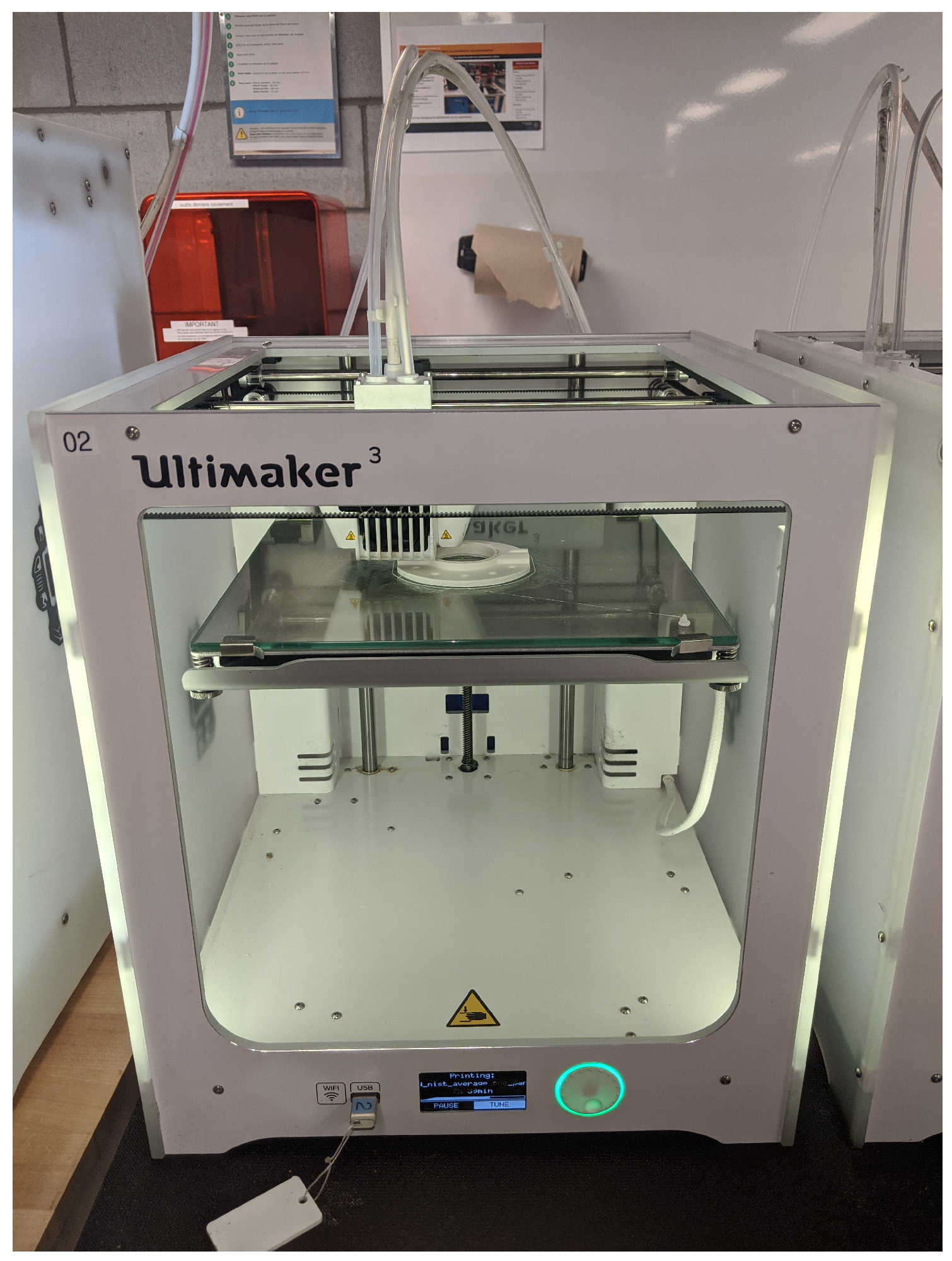
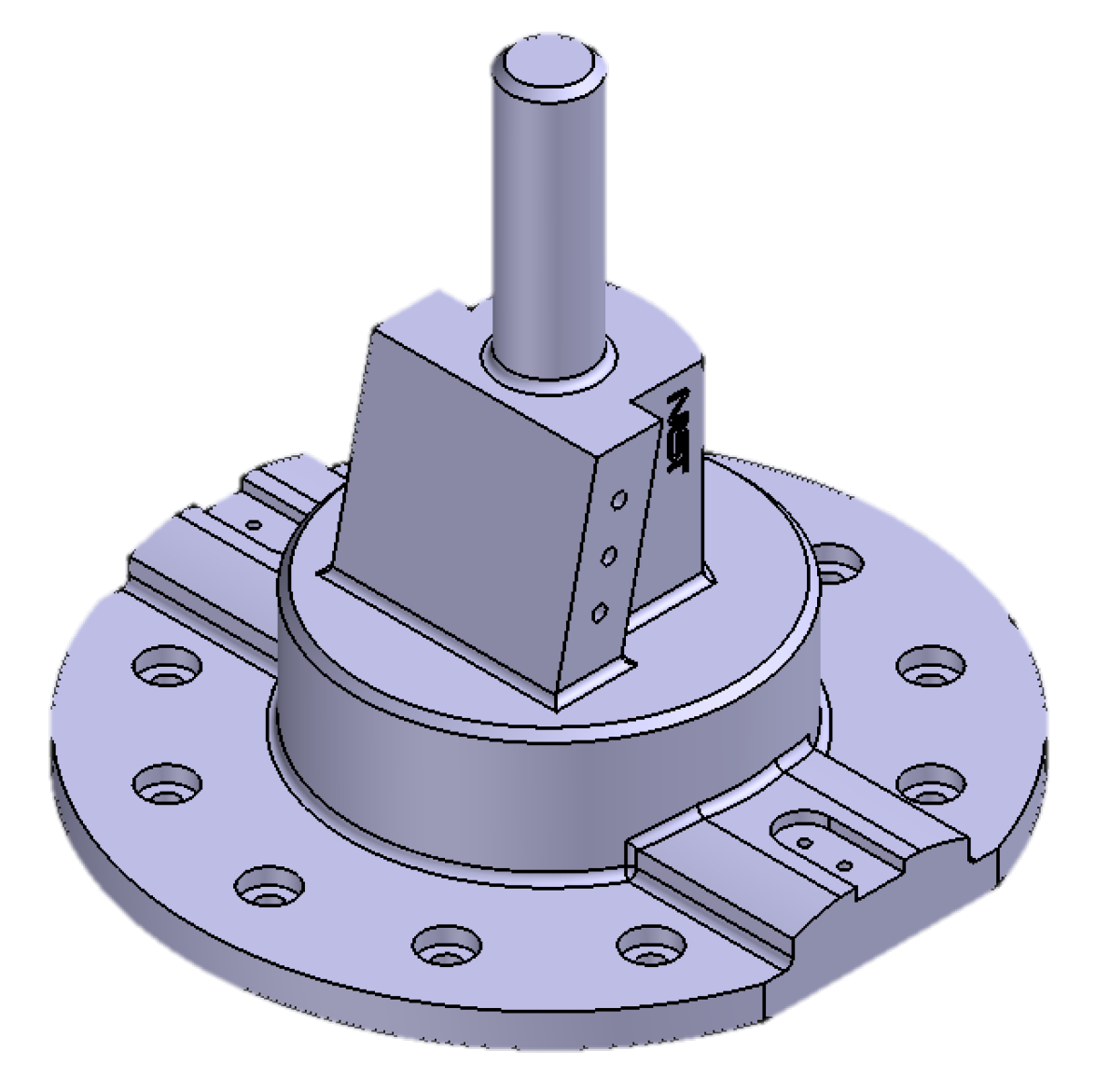
To verify the effectiveness of the proposed method, we printed a test part of the National Institute of Standards and Technology (NIST) five times using an Ultimaker 3 (Ultimaker, Geldermalsen, The Netherlands) 3D printer (Figure 2) with white 2.75 mm PLA filament from Ultimaker. The adopted part is CTC 5 [33], shown in Figure 3. The part was scaled uniformly to a reasonable size to print. The outside dimensions of the part are mm. CATIA allows the export of the part’s CAD model in the STL file format by imposing a step (i.e., maximum edge length) and a maximum chord deviation. In this work, the step was set at mm and the maximum chord deviation at mm. This allowed to minimize the deviation between the STL and the original CAD model and make it negligible in our experiment [34]. The exported STL model was sliced using Ultimaker Cura with the fast default profile and the layer height set to mm. With the negligible part file errors, the deviations of the printed part are mostly due to the machine’s imprecision and the material shrinkage. Table 1 presents the process parameters used for printing the original and compensated parts.
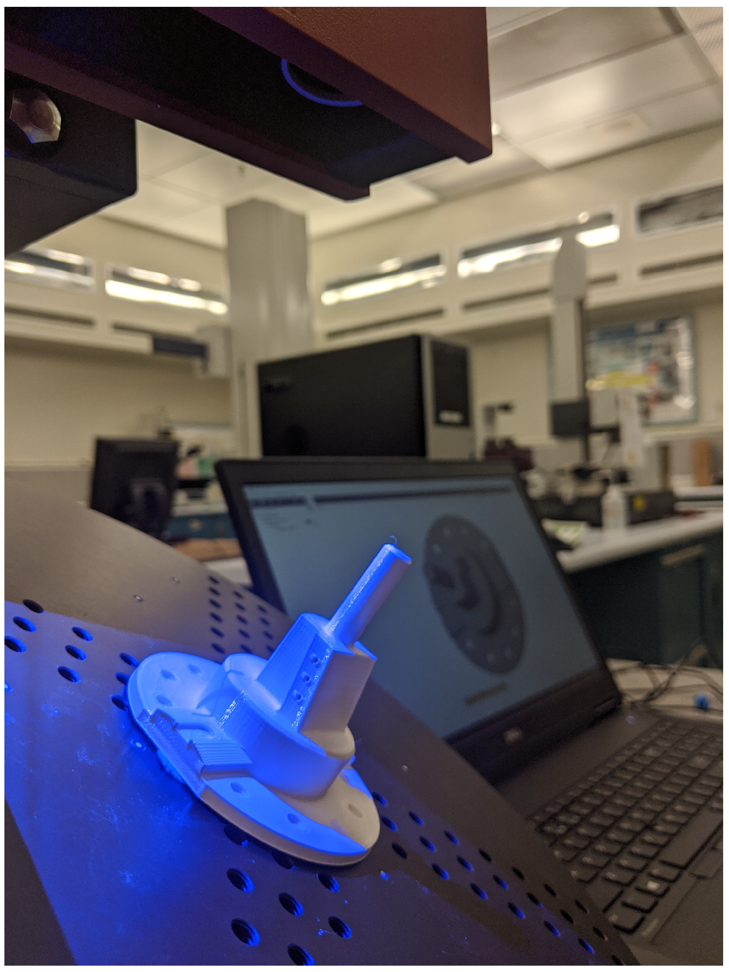
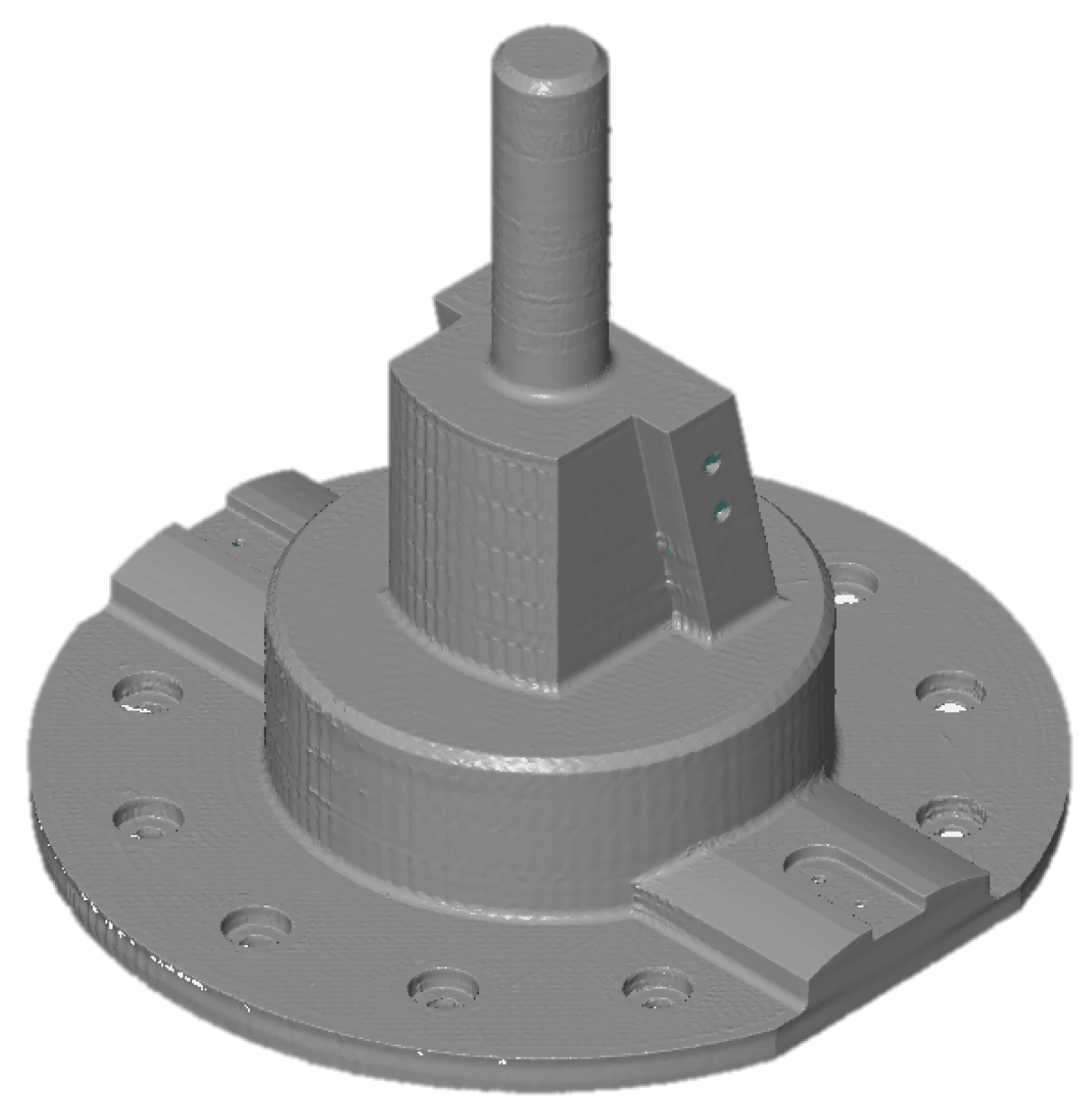
Each printed part was visually inspected first to make sure that no burrs, stray filaments, or major defects were present and then scanned using an ATOS Core 200 (GOM, Braunschweig, Germany) 3D scanner (Figure 4). The scan data are then exported from GOM Scan (the scanner’s data acquisition software). The resulting scan data are made of about 300,000 points at a density of . The scanner is able to detect every detail on the surface of the part, even the track of the printer’s nozzle (Figure 5). However, the holes on the sides and the bottom are harder to scan. A study of the 3D scanner’s accuracy in [35] demonstrated an accuracy of 10 m in length measurement and, more interestingly for us, 2 m in the probing error of form measurement.
3.2. Comparative Analysis
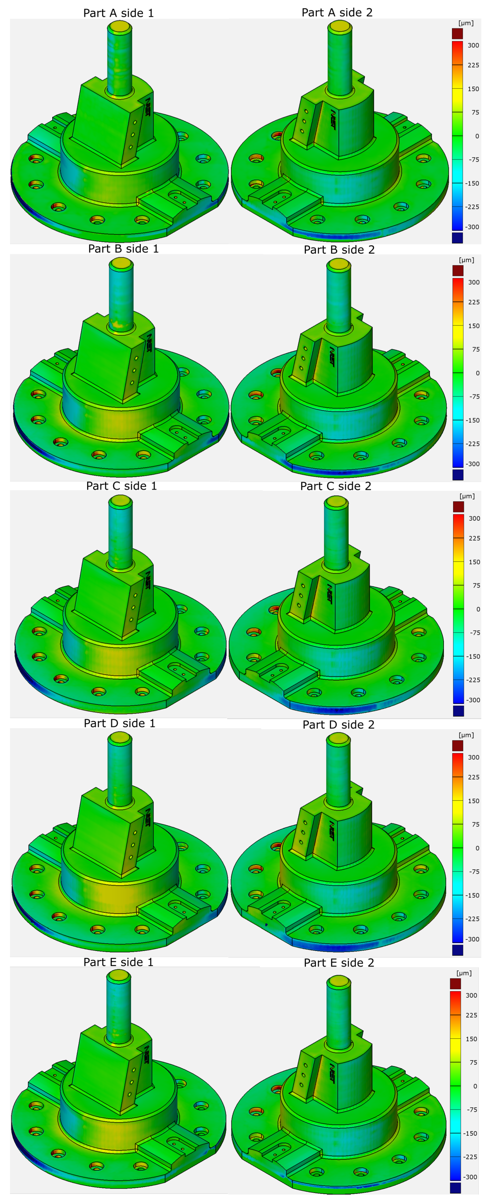
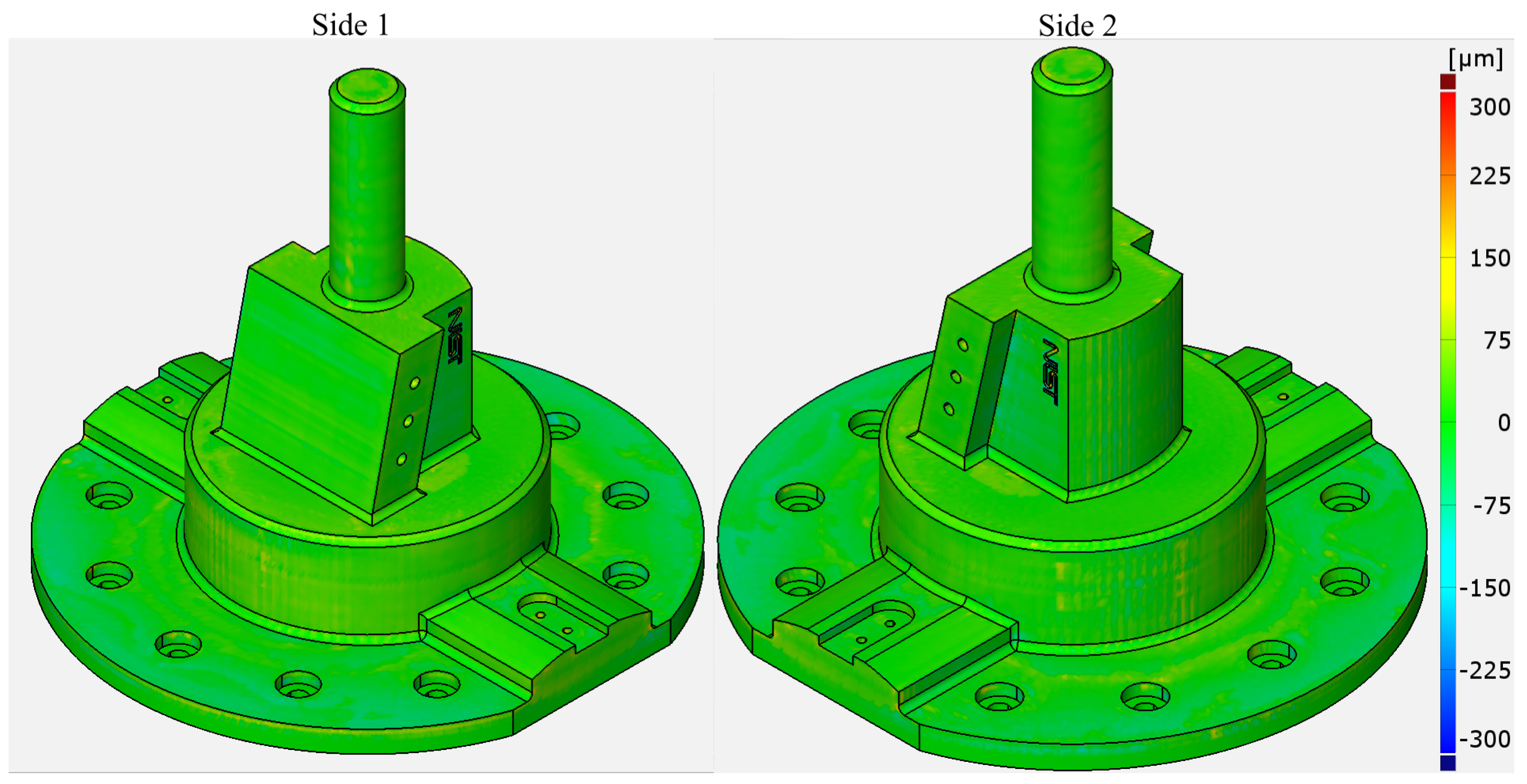
The comparison between the scan data of each printed part and the original CAD model yields the geometric deviation of the part. The colormaps of the deviations of the five printed parts (A–E) with respect to the original CAD model is presented in Figure 6. The deviation values on the colormaps are signed -norms of the deviation vectors. The sign of these values represents the direction of the deviation. A negative value means the deviation vector points to the inside of the geometry and vice versa.
The results of Section 3.2.1 and Section 3.2.2 validate the proposed compensation approach using the average deviation obtained from five parts and compare it to the compensation based on only one part. To this end, two compensated parts are obtained and compared. The first one only uses the deviation vector field of Part B for its compensation. The deviation vector field obtained from the scan was smoothed by the presented Laplacian smoothing before the morphing. The selection of which part to use for the compensation was random so as to not affect the result. The second one uses the average of all of the five parts’ deviation vector fields as proposed in this paper.
3.2.1. Deviation Analysis
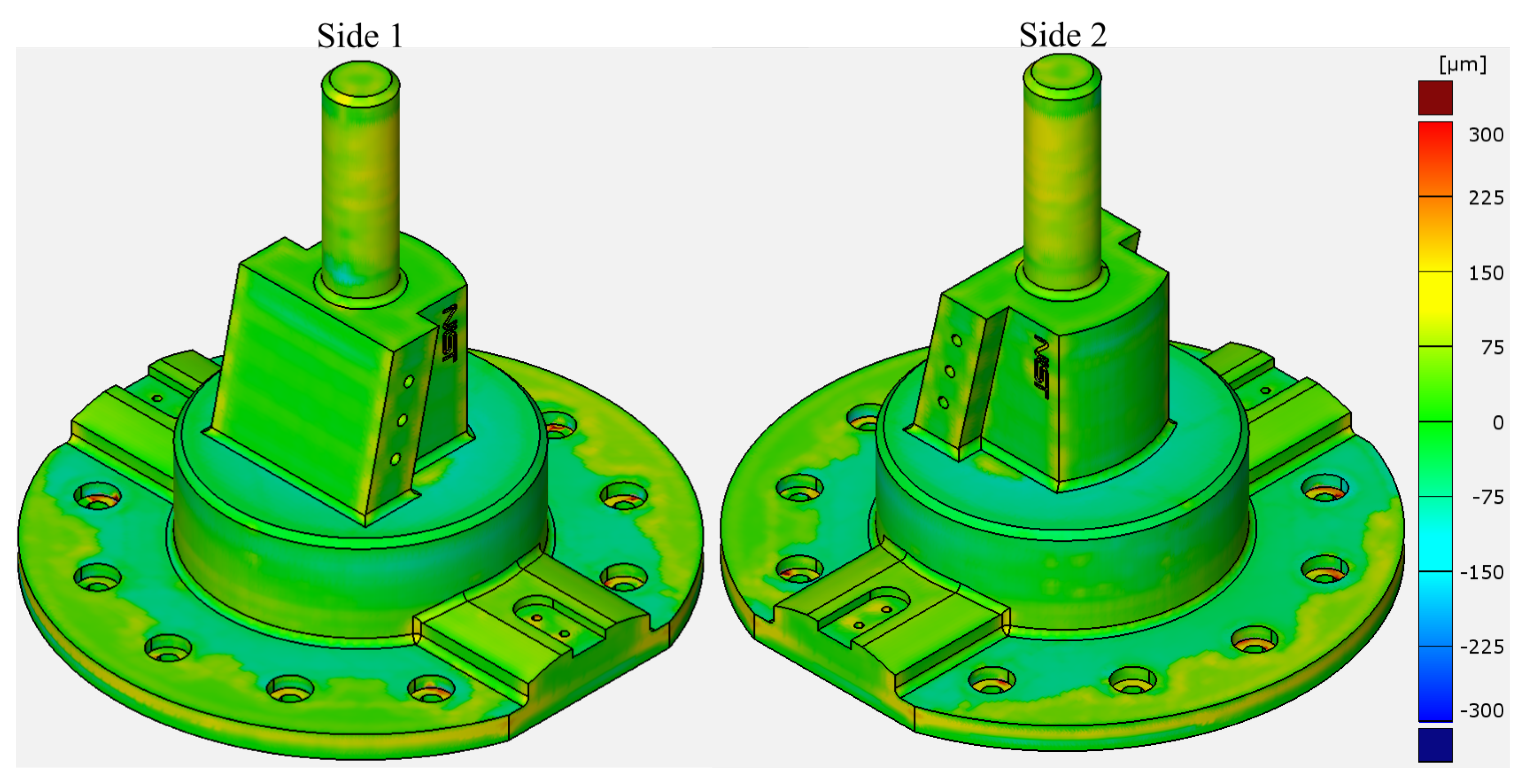
Part B, the part based on which the first compensated part was obtained, can be seen in Figure 6. It has an average absolute error of 53 m and a standard deviation of 60 m. The 99th percentile of the absolute errors is at 318 m. There is a clear deviation on the cylinders and other round features. There are some random deformations that are not repeated in other colormaps of Figure 6 (e.g., the yellow patch at the bottom of the top cylinder). The compensated part based on these deviations is displayed in Figure 7.
The average absolute error of this compensated part is 52 m and the standard deviation is 48 m. The 99th percentile is at 221 m. Compared to Part B, the average absolute error of the compensated part shows no improvement, but the standard deviation and the 99th percentile show an improvement of and , respectively.
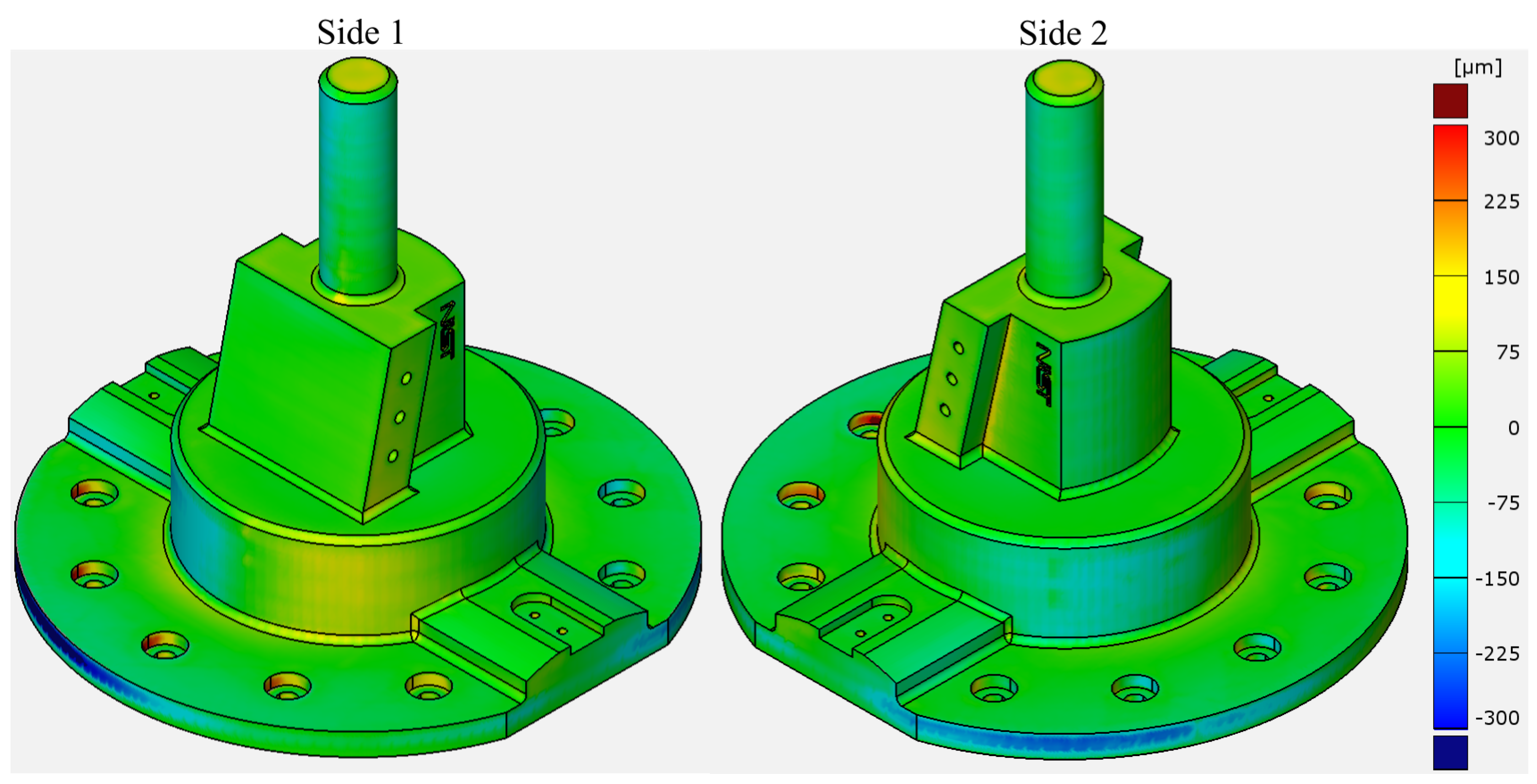
Table 2 presents the values of the average of absolute errors, standard deviation, and the 99th percentile of absolute errors for each of the five initial parts and the two compensated parts. The average absolute error of all the five original parts (of Figure 6) combined is 51 m with a standard deviation of 57 m. The average 99th percentile is at 311 m. It can be observed in Figure 6 that the deformation on the cylinders is present in every colormap, with a slight difference between them. It is then clear that there is a systematic deviation there that should be eliminated. The average deviation colormap and the standard deviation colormap are displayed in Figure 8 and Figure 9. The average colormap shows deformation patterns similar to the ones on each individual part of Figure 6. The low values on the standard deviation colormap confirm that the manufacturing process typically causes similar deviations in the same regions of the part.
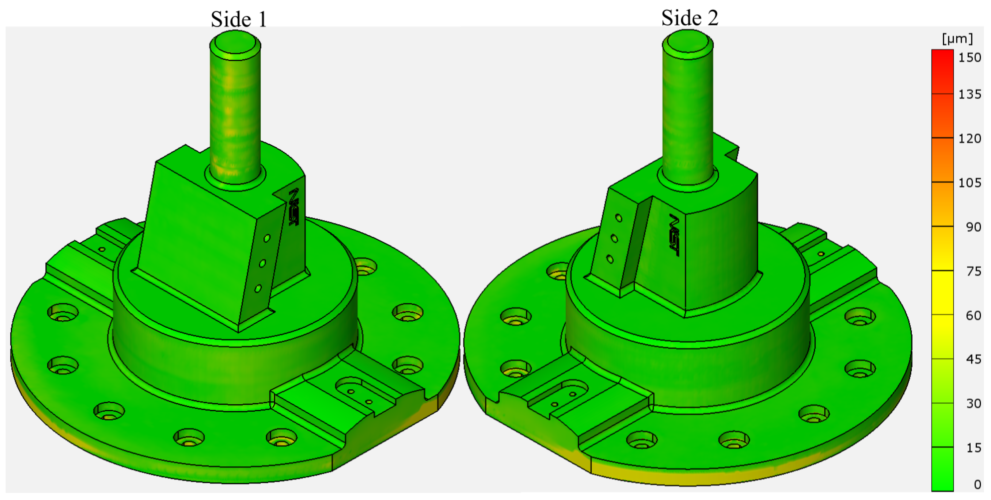
The compensated part based on the average of the five original parts is presented in Figure 10. It is clear that the cylinders show no deviations like the original parts and the deviations are smaller on the horizontal surfaces. The average absolute error of the compensated part is 23 m and the standard deviation is 20 m. The 99th percentile is at 98 m. These are an improvement of , , and , respectively.
Random deviations are still clearly visible on the compensated part. These are, in part, from the manufacturing of the compensated part and the measurement, but also from the random deviations that are non-negligible in the average deviation vector field and are included in the compensation.
3.2.2. Tolerance Analysis
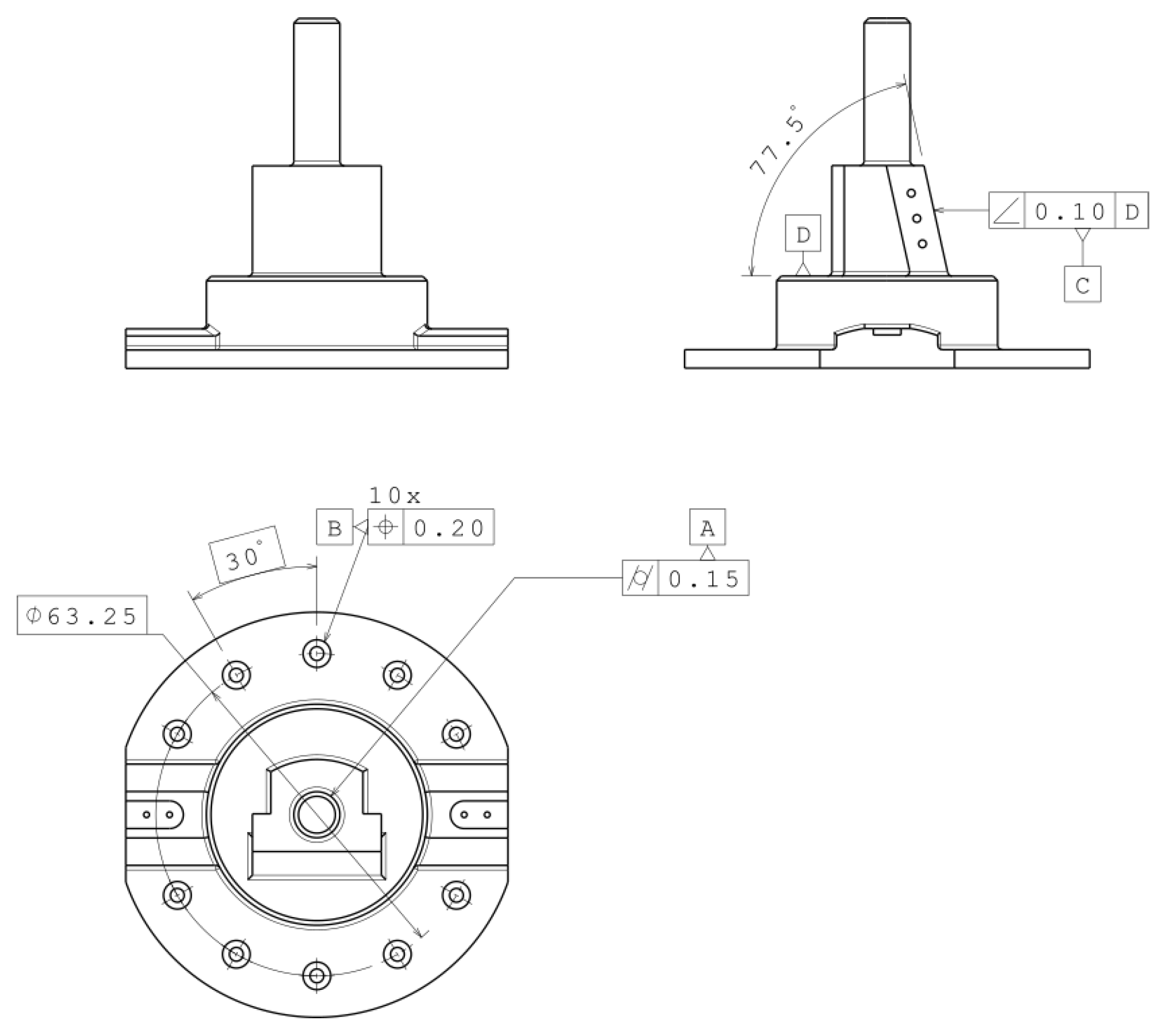
A Geometric Dimensioning and Tolerancing (GD&T) analysis is also performed, using GOM Inspect software, on each printed part. The tolerance features can be identified in the drawing of Figure 11. The tolerances are not the ones originally defined on NIST CTC 5 part. We have specified these tolerances merely for the sake of case studies of this paper. The standard used for tolerancing is the ASME Y14.5 2018 [38]. As it can be seen in Figure 11, the cylindricity tolerance is defined for cylinder A, the position tolerance is specified for the centroid of the 10 holes on the bottom surface, named as element group B, and the angularity tolerance is defined for plane C with respect to plane D as datum.
Table 3 presents the specified tolerance values for each of these tolerances and the corresponding deviation values obtained from the scan of each of the printed parts, namely, the initial five parts (A–E) and the two compensated parts.
It can be seen in Table 3 that the five original parts (A–E) are out of tolerance for all three features. The compensated part based on part B is out-of-tolerance for two tolerances. Cylinder A is out of tolerance because the compensation included a random deviation from part B. The yellow patch mentioned earlier in Figure 6 was compensated; its inverse, a blue patch, is visible in Figure 7. This patch, as it is not a high-frequency error, was not filtered by the Laplacian smoothing.
Finally, it can be seen in Table 3 that the compensated part based on the average deviation of the five original parts is in-tolerance for all inspected features. The compensation is clearly effective in removing deviations on cylindrical shapes. The reduction in cylindricity deviation, compared to the average of the five original parts is 51% for cylinder A. The position deviation of holes B is reduced by 61% and the angular deviation for plane C is reduced by 15%.
4. Conclusions
The proposed method of surface mesh compensation based on 3D metrology feedback adjusts the CAD model to oppose systematic deviations. The main sources of these deviations are material shrinkage and residual stress-induced deformations, as well as the positioning errors of the machine. We proposed the compensation based on the average deviation vector field obtained from the scans of multiple printed parts to ensure that the compensation is performed only for the repeated systematic deviations and not the random deviations of a single part. The use of an optical 3D scanner allows for quick digitization of the printed parts. Local deviations can be easily measured since a high-density point cloud is obtained through optical 3D scanning. The presented Laplacian smoothing can filter out the high-frequency noise of the scans.
The case study results confirm that random deviations have an adverse impact on the compensation outcome if not mitigated by compensating based on the average deviation of multiple parts. The compensation based on the deviation of only one part shows a lower capacity to reduce deviations as the improvement of geometrical accuracy was only 31%. This was not enough to bring the deviations of the compensated part within all specified tolerances.
The proposed approach of compensation based on the average of five parts is able to improve geometrical accuracy by 68% based on the 99th percentile of absolute deviations. The proposed compensation based on the average of five parts could successfully bring the deviations of the compensated part within the specified tolerance values.
Author Contributions
Conceptualization, M.J. and F.K.; methodology, M.J. and F.K.; software, M.J.; validation, M.J.; formal analysis, M.J. and F.K.; investigation, M.J.; resources, M.J. and F.K.; data curation, M.J.; writing—original draft preparation, M.J.; writing—review and editing, M.J. and F.K.; visualization, M.J.; supervision, F.K.; project administration, F.K.; funding acquisition, F.K. All authors have read and agreed to the published version of the manuscript.
Funding
This research was supported by the Fonds de Recherche du Québec—Nature et Technologies (FRQNT).
Conflicts of Interest
The authors declare no conflict of interest.
Abbreviations
The following abbreviations are used in this manuscript:
| AM | Additive Manufacturing |
| PPE | Personal Protective Equipment |
| FDM | Fused Deposition Modelling |
| FFF | Fused Filament Fabrication |
| SLA | Stereolithography Apparatus |
| CAD | Computer Aided Design |
| FEA | Finite Element Analysis |
| ICP | Iterative Closest Point |
| STL | Standard Tessellation Language |
| GD&T | Geometric Dimensioning and Tolerancing |
| CMM | Coordinate Measuring Machine |
References
- Sachs, E.; Cima, M.; Williams, P.; Brancazio, D.; Cornie, J. Three Dimensional Printing: Rapid Tooling and Prototypes Directly from a CAD Model. J. Eng. Ind. 1992, 114, 481–488. [Google Scholar] [CrossRef]
- Gao, W.; Zhang, Y.; Ramanujan, D.; Ramani, K.; Chen, Y.; Williams, C.B.; Wang, C.C.L.; Shin, Y.C.; Zhang, S.; Zavattieri, P.D. The status, challenges, and future of additive manufacturing in engineering. Comput. Aided Des. 2015, 69, 65–89. [Google Scholar] [CrossRef]
- Msallem, B.; Sharma, N.; Cao, S.; Halbeisen, F.S.; Zeilhofer, H.F.; Thieringer, F.M. Evaluation of the Dimensional Accuracy of 3D-Printed Anatomical Mandibular Models Using FFF, SLA, SLS, MJ, and BJ Printing Technology. J. Clin. Med. 2020, 9, 817. [Google Scholar] [CrossRef] [PubMed] [Green Version]
- Manero, A.; Smith, P.; Koontz, A.; Dombrowski, M.; Sparkman, J.; Courbin, D.; Chi, A. Leveraging 3D Printing Capacity in Times of Crisis: Recommendations for COVID-19 Distributed Manufacturing for Medical Equipment Rapid Response. Int. J. Environ. Res. Public Health 2020, 17, 4634. [Google Scholar] [CrossRef] [PubMed]
- Pearce, J.M. Distributed Manufacturing of Open Source Medical Hardware for Pandemics. J. Manuf. Mater. Process. 2020, 4, 49. [Google Scholar] [CrossRef]
- Bochmann, L.; Bayley, C.; Helu, M.; Transchel, R.; Wegener, K.; Dornfeld, D. Understanding error generation in fused deposition modeling. Surf. Topogr. Metrol. Prop. 2015, 3, 014002. [Google Scholar] [CrossRef]
- Akinsowon, V.; Nahirna, M. State of the 3D Printing Industry Survey 2019: AM Service Providers. Available online: https://amfg.ai/wp-content/uploads/2019/07/AMFG-State-of-the-Industry-Report_-AM-Service-Providers.pdf (accessed on 19 November 2020).
- Gibson, I.; Rosen, D.W.; Stucker, B. Additive Manufacturing Technologies: 3D Printing, Rapid Prototyping, and Direct Digital Manufacturing; Springer: Berlin/Heidelberg, Germany, 2016. [Google Scholar]
- Yang, H.J.; Hwang, P.J.; Lee, S.H. A study on shrinkage compensation of the SLS process by using the Taguchi method. Int. J. Mach. Tools Manuf. 2002, 42, 1203–1212. [Google Scholar] [CrossRef]
- Karalekas, D.; Aggelopoulos, A. Study of shrinkage strains in a stereolithography cured acrylic photopolymer resin. J. Mater. Process. Technol. 2003, 136, 146–150. [Google Scholar] [CrossRef]
- Wang, T.M.; Xi, J.T.; Jin, Y. A model research for prototype warp deformation in the FDM process. Int. J. Adv. Manuf. Technol. 2007, 33, 1087–1096. [Google Scholar] [CrossRef]
- Bourell, D.; Kruth, J.P.; Leu, M.; Levy, G.; Rosen, D.; Beese, A.M.; Clare, A. Materials for additive manufacturing. CIRP Ann. 2017, 66, 659–681. [Google Scholar] [CrossRef]
- Tong, K.; Amine Lehtihet, E.; Joshi, S. Parametric error modeling and software error compensation for rapid prototyping. Rapid Prototyp. J. 2003, 9, 301–313. [Google Scholar] [CrossRef]
- Tong, K.; Lehtihet, E.A.; Joshi, S. Software compensation of rapid prototyping machines. Precis. Eng. 2004, 28, 280–292. [Google Scholar] [CrossRef]
- Tong, K.; Joshi, S.; Amine Lehtihet, E. Error compensation for fused deposition modeling (FDM) machine by correcting slice files. Rapid Prototyp. J. 2008, 14, 4–14. [Google Scholar] [CrossRef]
- Lyu, J.; Manoochehri, S. Modeling Machine Motion and Process Parameter Errors for Improving Dimensional Accuracy of Fused Deposition Modeling Machines. J. Manuf. Sci. Eng. 2018, 140. [Google Scholar] [CrossRef]
- Huang, Q.; Nouri, H.; Xu, K.; Chen, Y.; Sosina, S.; Dasgupta, T. Statistical Predictive Modeling and Compensation of Geometric Deviations of Three-Dimensional Printed Products. J. Manuf. Sci. Eng. 2014, 136, 061008. [Google Scholar] [CrossRef]
- Huang, Q.; Zhang, J.; Sabbaghi, A.; Dasgupta, T. Optimal offline compensation of shape shrinkage for three-dimensional printing processes. IIE Trans. 2015, 47, 431–441. [Google Scholar] [CrossRef]
- Huang, Q. An Analytical Foundation for Optimal Compensation of Three-Dimensional Shape Deformation in Additive Manufacturing. J. Manuf. Sci. Eng. 2016, 138, 061010. [Google Scholar] [CrossRef]
- Huang, Q.; Wang, Y.; Lyu, M.; Lin, W. Shape Deviation Generator—A Convolution Framework for Learning and Predicting 3D Printing Shape Accuracy. IEEE Trans. Autom. Sci. Eng. 2020, 17, 1486–1500. [Google Scholar] [CrossRef]
- Chowdhury, S.; Mhapsekar, K.; Anand, S. Part Build Orientation Optimization and Neural Network-Based Geometry Compensation for Additive Manufacturing Process. J. Manuf. Sci. Eng. 2018, 140. [Google Scholar] [CrossRef]
- McConaha, M.; Anand, S. Additive Manufacturing Distortion Compensation Based on Scan Data of Built Geometry. J. Manuf. Sci. Eng. 2020, 142. [Google Scholar] [CrossRef]
- Xu, K.; Kwok, T.H.; Zhao, Z.; Chen, Y. A Reverse Compensation Framework for Shape Deformation Control in Additive Manufacturing. J. Comput. Inf. Sci. Eng. 2017, 17, 021012. [Google Scholar] [CrossRef]
- Afazov, S.; Okioga, A.; Holloway, A.; Denmark, W.; Triantaphyllou, A.; Smith, S.A.; Bradley-Smith, L. A methodology for precision additive manufacturing through compensation. Precis. Eng. 2017, 50, 269–274. [Google Scholar] [CrossRef]
- Grimm, T. Users Guide to Rapid Prototyping; Society of Manufacturing Engineers: Dearborn, MI, USA, 2004. [Google Scholar]
- Besl, P.J.; McKay, N.D. A method for registration of 3D shapes. IEEE Trans. Pattern Anal. Mach. Intell. 1992, 14, 239–256. [Google Scholar] [CrossRef]
- Dowllng, M.M.; Griffin, P.M.; Tsui, K.L.; Zhou, C. Statistical issues in geometric feature inspection using coordinate measuring machines. Technometrics 1997, 39, 3. [Google Scholar] [CrossRef]
- Weyrich, T.; Pauly, M.; Keiser, R.; Heinzle, S.; Scandella, S.; Gross, M. Post-Processing of Scanned 3D Surface Data. In Proceedings of the First, Eurographics Conference on Point-Based Graphics, Zurich, Switzerland, 2–4 June 2004; pp. 85–94. [Google Scholar]
- Desbrun, M.; Meyer, M.; Schröder, P.; Barr, A.H. Implicit fairing of irregular meshes using diffusion and curvature flow. In Proceedings of the 26th Annual Conference on Computer Graphics and Interactive Techniques—SIGGRAPH 99, Los Angeles, CA, USA, 8–13 August 1999. [Google Scholar] [CrossRef] [Green Version]
- Sharp, N.; Soliman, Y.; Crane, K. The Vector Heat Method. ACM Trans. Graph. 2019, 38, 24:1–24:19. [Google Scholar] [CrossRef]
- Bunge, A.; Herholz, P.; Kazhdan, M.; Botsch, M. Polygon Laplacian Made Simple. Comput. Graph. Forum 2020, 39, 303–313. [Google Scholar] [CrossRef]
- Minetola, P.; Calignano, F.; Galati, M. Comparing geometric tolerance capabilities of additive manufacturing systems for polymers. Addit. Manuf. 2020, 32, 101103. [Google Scholar] [CrossRef]
- Lipman, R.; Filliben, J. Testing Implementations of Geometric Dimensioning and Tolerancing in CAD Software. Comput. Aided Des. Appl. 2020, 17, 1241–1265. [Google Scholar] [CrossRef]
- Navangul, G.; Paul, R.; Anand, S. Error Minimization in Layered Manufacturing Parts by Stereolithography File Modification Using a Vertex Translation Algorithm. J. Manuf. Sci. Eng. 2013, 135. [Google Scholar] [CrossRef]
- Acceptance/Reverification According to VDI/VDE 2634, Part 3. Available online: https://www.zebicon.com/fileadmin/user_upload/2_Maaleudstyr/9_Certifikater/ATOS_Core_200_SN160300/2019-04-02_Acceptance_test_ATOS_Core_MV200_SN160300.pdf (accessed on 19 November 2020).
- Dawson-Haggerty, M. Trimesh. 2019. Available online: https://trimsh.org/ (accessed on 30 June 2020).
- Jacobson, A.; Panozzo, D. libigl: A Simple C++ Geometry Processing Library. 2018. Available online: https://libigl.github.io/ (accessed on 15 September 2020).
- ASME Y14.5—2018: Dimensioning and Tolerancing; American Society of Mechanical Engineers: New York, NY, USA, 2018.
Figure 1.
Outline of the proposed 3D compensation.

Figure 2.
Ultimaker 3, 3D printing the part in PLA.

Figure 3.
NIST CTC 5 CAD model.

Figure 4.
3D scanning setup with ATOS Core.

Figure 5.
Scan data of the printed part.

Figure 6.
Deviation colormaps of the five original printed parts, ranges are in m.

Figure 7.
Deviation colormap of the compensated part based on part B, range is in m.

Figure 8.
Average deviation colormap of the five original printed parts, range is in m.

Figure 9.
Standard deviation colormap of the five original printed parts, range is in m.

Figure 10.
Deviation colormap of the compensated part based on the average of five parts, range is in m.
Figure 10.
Deviation colormap of the compensated part based on the average of five parts, range is in m.

Figure 11.
Drawing of the part with the toleranced features to inspect. Unless otherwise specified, dimensions are in mm.
Figure 11.
Drawing of the part with the toleranced features to inspect. Unless otherwise specified, dimensions are in mm.


Table 1.
Printing parameters for the original and compensated parts.
| Printing temperature | 215 °C |
| Printing speed | 70 mm/s |
| Cooling | 100% |
| Support | None |
| Infill type | Triangles |
| Infill density | 10% |
| Plate adhesion | None |
| Layer height | 0.04 mm |
| Nozzle diameter | 0.4 mm |
Table 2.
Average of absolute errors, standard deviation, and 99th percentile of absolute errors of the original five parts (A–E) and the two compensated parts.
Table 2.
Average of absolute errors, standard deviation, and 99th percentile of absolute errors of the original five parts (A–E) and the two compensated parts.
| Average of Absolute Errors (m) | Standard Deviation (m) | 99th Percentile of Absolute Errors (m) | |
|---|---|---|---|
| Compensated part based on the average deviation of 5 parts | 23 | 20 | 98 |
| Compensated part based on deviation of part B | 52 | 48 | 221 |
| Part A | 52 | 62 | 330 |
| Part B | 53 | 60 | 318 |
| Part C | 51 | 57 | 309 |
| Part D | 49 | 54 | 288 |
| Part E | 48 | 54 | 309 |
Table 3.
The values of the specified tolerances on the part, and the corresponding deviation values obtained from the scans for each of the five initial parts, the compensated part based on part B, and the compensated part based on the average of five parts. The values are in m.
Table 3.
The values of the specified tolerances on the part, and the corresponding deviation values obtained from the scans for each of the five initial parts, the compensated part based on part B, and the compensated part based on the average of five parts. The values are in m.
| Element | Cylinder A | Element Group B | Plane C |
|---|---|---|---|
| Datum | Plane D | ||
| Property | Cylindricity | Position | Angularity |
| Tolerance | 150 | 200 | 100 |
| Deviation of Compensated part based on the average deviation of five parts | 125 | 179 | 98 |
| Deviation of Compensated part based on part B | 165 | 194 | 156 |
| Deviation of part A | 285 | 499 | 108 |
| Deviation of part B | 282 | 455 | 103 |
| Deviation of part C | 244 | 499 | 117 |
| Deviation of part D | 179 | 502 | 125 |
| Deviation of part E | 273 | 471 | 122 |
Publisher’s Note: MDPI stays neutral with regard to jurisdictional claims in published maps and institutional affiliations. |
© 2020 by the authors. Licensee MDPI, Basel, Switzerland. This article is an open access article distributed under the terms and conditions of the Creative Commons Attribution (CC BY) license (http://creativecommons.org/licenses/by/4.0/).
Share and Cite
MDPI and ACS Style
Jadayel, M.; Khameneifar, F. Improving Geometric Accuracy of 3D Printed Parts Using 3D Metrology Feedback and Mesh Morphing. J. Manuf. Mater. Process. 2020, 4, 112. https://0-doi-org.brum.beds.ac.uk/10.3390/jmmp4040112
AMA Style
Jadayel M, Khameneifar F. Improving Geometric Accuracy of 3D Printed Parts Using 3D Metrology Feedback and Mesh Morphing. Journal of Manufacturing and Materials Processing. 2020; 4(4):112. https://0-doi-org.brum.beds.ac.uk/10.3390/jmmp4040112
Chicago/Turabian StyleJadayel, Moustapha, and Farbod Khameneifar. 2020. "Improving Geometric Accuracy of 3D Printed Parts Using 3D Metrology Feedback and Mesh Morphing" Journal of Manufacturing and Materials Processing 4, no. 4: 112. https://0-doi-org.brum.beds.ac.uk/10.3390/jmmp4040112