Article

Characterization of the Morphological Behavior of a Sand Spit Using UAVs

by
Alejandro Paladio-Hernandez
1,
Paulo Salles
1,2,*,
Jaime Arriaga
3 and
José López-González
1,2
1
Laboratorio de Ingenieria y Procesos Costeros, Instituto de Ingenieria, UNAM, Ciudad de Mexico 04510, Mexico
2
Laboratorio Nacional de Resiliencia Costera, Laboratorios Nacionales (LANRESC) CONACYT, Sisal 97356, Mexico
3
Faculty of Civil Engineering and Geosciences, Delft University of Technology, 2628 CN Delft, The Netherlands
*
Author to whom correspondence should be addressed.
J. Mar. Sci. Eng. 2022, 10(5), 600; https://0-doi-org.brum.beds.ac.uk/10.3390/jmse10050600
Submission received: 11 March 2022 / Revised: 18 April 2022 / Accepted: 19 April 2022 / Published: 29 April 2022

Abstract

:
Sand spits are common in wave-dominated environments; with enough sand supply, they can evolve to affect circulation and navigation in channels or inlets. The focus of this paper is on the navigation channel of the Sisal Port, located on the northwestern Yucatan Peninsula (YP) coast, where a sand spit grew and was monitored from its formation (June 2018) until navigation was practically blocked (November 2018). The YP coast is characterized as being microtidal, with significant wave heights ranging from 0.1 to 0.4 m (April to September), and in the presence of high energy events (cold fronts and storms), waves can reach heights of up to 2.5 m offshore at 10 m depth (October to February). Prior to the beginning of UAV surveys, we used photos (June–July 2018) from a stationary field camera and hydrodynamic data from models (WaveWatch III for waves and MARV software for tidal levels) to generate a qualitative description of the sand spit in the channel. Combining products from UAVs flights (DEMs) and hydrodynamic measurements (wave energy flux), we characterized the behavior and response of the sand spit, from its formation near the jetty head, through its consolidation in October 2018, to when a cold front with HS ∼2.5 m breached it in mid-November. The results show that spit formation takes place during calm conditions (e.g., periods dominated by sea breezes), and depending on the energy threshold of high energetic events, this new spit will consolidate or be breached. Migration of the spit is related to overwash events and changes in wave direction. The presented methodology provides a well-rounded tool for characterizing the morphological behavior of spits on a shallow coast, which can be useful for improving coastal management.
Keywords:
sand spit; UAV; inlet; harbor

1. Introduction

The feedback between hydrodynamics and morphology shapes the coast. Continuous positive feedback can develop coherent sand structures, while negative feedback tends to diffuse them. These can be observed above water level (e.g., dunes, spits), at the shoreline (e.g., cusps, megacusps, shoreline sand waves), and below water level (e.g., ripples, sandbars) at different space and time scales [1,2].
Spits are common when the coastline presents abrupt changes and longshore transport has a dominant direction creating a converging sediment zone, e.g., downdrift from a jetty or tidal inlet [3,4]. Sand spit growth and evolution are driven by many factors, including an underlying geological framework [5], wave processes [6,7,8], wave approaching angle [9,10,11], swash bar welding [12,13], tidal currents [13], longshore sediment drift [3,14], and overwash events [15,16]. Each process leads to a specific development (or degeneration, e.g., overwash events) of spit geometric characteristics.
The presence of a sand spit can have negative effects; for example, Wiegel [17] and Komar and Moore [18] mentioned possible negative effects of sand spit development between jetties, which results in waterway blockage, thus affecting navigability and fishery capability, increasing the residence water time, and reducing water quality. Considering the problems a spit can cause, an analytical solution was developed by Kraus (1999) [3] for port channels and tidal inlets, considering spit elongation. In addition, inlet closure by spit was considered by Ogawa (1984) [19] and Tanaka (1995) [20].
Monitoring changes in sand spits, together with the varying hydrodynamic conditions, helps develop a better understanding of the sand structure dynamics and improve coastal management. The classic way of monitoring the beach is through in situ measurements (e.g., on-foot or vehicle DGPS single-antenna systems), which are accurate but limit the spatiotemporal scale of the monitoring. Technological advancements have allowed us to use noninvasive techniques (e.g., satellites, unmanned aerial vehicles, or fixed field cameras and GPS measurements), covering large areas but sacrificing accuracy. A combination of both systems has been employed with encouraging results (e.g., [21]). Duy et al. [22] used 40 satellite images to monitor a sand spit over 44 years, having coarse pixel resolution (i.e., mainly 60 and 30 m/pixel). Sasaki and Sato [23] monitored the morphological changes of a sand spit using a field camera and obtained one image every 120 s over 14 months, capturing changes in the sand spit during normal and storm conditions. These two studies were conducted in river mouths. Long et al. (2016) [24] used three UAV surveys over 5 months to monitor changes in a tidal inlet, in which the development of a sand spit occurred.
In the last 30 years, 12 small ports have been developed in the Yucatan Peninsula; these were developed without considering the morphological effects due to wave and tidal climate [25]. The aim of this paper is to evaluate the growth and evolution of the sand spit at the port of Sisal using (a) fixed-camera and orthorectified UAV imagery compared to on-foot DGPS measurements, (b) the cumulative wave energy flux, and (c) cumulative longshore sediment transport during the study time periods. In Section 2, we present how and when we measured the sand spit and the hydrodynamic conditions while the spit was present, as well as the type of equipment we used. Section 3 presents the evolution of the spit and how it is linked to the current hydrodynamic conditions, which helps in understanding morphological changes (e.g., enlargement, decrement, migration, and changes during storm conditions). In Section 4 and Section 5, discussions and conclusions are presented.

2. Materials and Methods
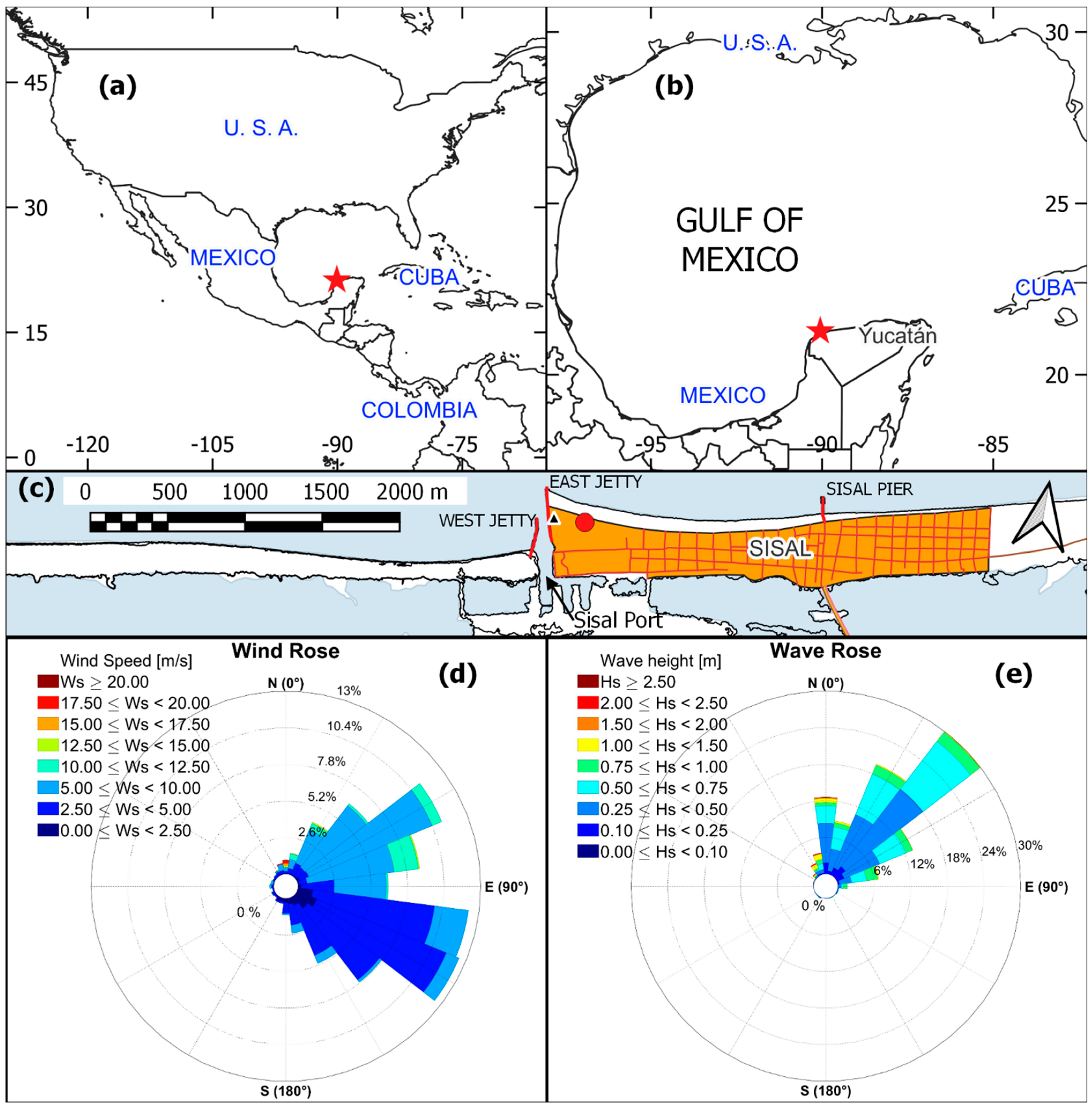
2.1. Study Site

The northern coast of the Yucatan Peninsula (YP), located between the Caribbean Sea and the Gulf of Mexico (Figure 1a), is characterized as having a shallow continental shelf up to 250 km wide, with a consistent smooth slope of around 0.001 (i.e., a depth of ~10 m is found 10 km offshore), over which the Yucatan current flows [26]. A net longshore sediment transport (LST) towards the west is present [27,28]. The northern YP has 12 small shelter ports (with one channel and widths over 70 m protected by two jetties) that are intended for fishing activities and tourism. To the authors’ knowledge, these ports all suffer from sand blockage. This has been reported by Franklin et al. (2021) [25] for the port of Sisal where siltation is a problem since there are no robust preventive coastal management plans, and the channel is dredged until navigation and ecological problems are generated due to this blockage.
The northern coast of Yucatan is a barrier island with a length of approximately 350 km. Freshwater is discharged to the coast via the confined aquifer groundwater in the form of submarine springs [29], as well as springs in coastal lagoons and wetlands [30]. The port of Sisal, located on the northwestern side of the Yucatan Peninsula (Figure 1b), was built with two jetties in 1987 [31] to maintain a ~66 m wide waterway (Figure 1c).
The beach has a mild slope [26] and an azimuthal angle of 70°, the surf zone is characterized by a sediment grain size ranging from 0.2 to 2.0 mm [32], and the predominant wave direction produces a net westward sediment transport [33]. The eastern and western jetties in Sisal have lengths of 350 m and 220 m, respectively, and the beach reached the eastern (longer) breakwater head on 17 June 2018 [33].
Spring and neap tidal ranges in the Yucatan peninsula are 0.80 m and 0.10 m, respectively, with a mixed regime and a diurnal predominance [33,34]. In addition, the monthly average mean sea level (MSL) fluctuates throughout the year, reaching its peak in October and its lowest value in July [33,35,36]. To calculate residual tide, the MARV software [37] was implemented, and an astronomical tide from the nearest point was predicted and subsequently subtracted from the measured tide.
In the study zone, there is a prevalence of local winds (sea and land breezes). Sea breezes have the most energetic conditions, with their daily peak reaching 10 m/s, and a predominant direction from the NE. Winter cold fronts (Central American cold surges (CACSs)), referred to locally as nortes, occur from September to March and bring dry polar air to the peninsula from the NNW–N, maintaining high-speed winds of more than 10 m.s−1 for more than 24 h during each event [28,38,39]. In the YP, sea breezes are present all year round, during which waves have an incident angle of ~45° and significant wave height below 0.8 m, with peak periods ranging from 3 s to 5 s. A CACS produces waves with an incident wave angle of −15° to 0°, a significant wave height over 2 m (data from an instrument at 10 m depth), and a peak period over 10 s.
The wetland in the back barrier, which in the area of Sisal is very shallow (20–30 cm depth), is mostly dry during the dry months and has a negligible water exchange with the port throughout the year. Given the small dimensions of the Sisal port water body (9.5 ha) and its shallow depth (1 m on average), the flood and ebb currents are weak on this microtidal coast, and therefore their impact on sediment transport and channel morphodynamics was not considered in this study. In addition, due to the frequent formation of sand deposits in the channel—sometimes in the form of spits like the one studied here—corrective (not preventive) dredging occurs in the channel and some also on the beach east of the channel (often months after the navigation becomes critical) to partially restore the jetty functionality in terms of retaining the westward longshore transport.

2.2. Waves and Alongshore Sediment Transport Characterization

Morphological changes in the coast are an effect of combined wind and water level oscillations and wave conditions. Atmospheric and oceanographic conditions are constantly monitored by the Laboratorio de Ingenieria y Procesos Costeros (LIPC) in the area [40] (data can be accessed through the web page http://ocse.mx/ accessed on 10 March 2022).
Wave and tidal conditions were measured using an RDI Sentinel Acoustic Doppler Velocimeter (ADCP; Manufacturer: RD Instruments, Poway, CA, USA) 12 km offshore of the Port of Sisal at 10 m water depth (Figure 1b), measuring significant wave height (HS), peak period (TP), peak wave direction (θW), and still water level (η) every 60 min. The ADCP did not measure wave direction during 5% of the study period (end of July 2018 to November 2018), and these gaps were filled with data from the WaveWatch III model (see red lines for HS and TP in Figure 2a,b and red circles in Figure 2c); data from this model were selected because they have previously shown a good correlation with measured data [41]. Wave data can be found at https://polar.ncep.noaa.gov/ accessed on 23 September 2019. To calculate the residual tide, we extracted the astronomical tidal signal from a nearby tide gage in Puerto Progreso (Lat: 21°18.20′, Lon: −89°40.00′), and then we subtracted this signal from the actual measured tide. Values obtained are presented in Figure 2d (red continuous line). Finally, wind data records were obtained from the meteorological station (Manufacturer: Campbell Scientific, Barcelona, Spain) of the National Autonomous University of Mexico (www.ruoa.unam.mx, accessed on 8 January 2019).
Offshore waves on the northwest coast of the Yucatan Peninsula show their lowest height and period from April to mid-September (HS < 0.5 m and 4 s < TP < 6 s) with waves coming from the NE, characteristic of sea breeze conditions, increasing to HS > 0.6 and TP > 6 s from mid-September to March [33]. The Central American cold surge (CACS) season (or norte season) occurs from September to March (HS > 2 m, TP > 10 s, and increase in MSL); CACSs are synoptic-scale events that arrive at the peninsula and last more than 24 h, driven only by cold and dry polar air [39]. Throughout these extreme events, the wave direction encompasses the NW–N sector.
To characterize the dominant wave conditions for each period (between surveys), waves were propagated using linear wave theory until breaking, considering the beach azimuthal angle of 70°. Subsequently, we calculated the cumulative cross-shore and alongshore component of the wave energy flux (Equations (1) and (2)) and the longshore sediment transport (LST) from CERC (Equation (3)), and the wave height and weighted average wave direction and peak period were computed at breaking point (see Table 1). LST from CERC [42] was calculated (m3/year) with hourly wave conditions, and then the values were accumulated by day to be subsequently divided by the measurement period to obtain the period mean value.
F bc = 2 5 / 4 8 * g 3 / 2 γ b * ρ H b 5 / 2 cos θ b
F bl = 2 5 / 4 8 * g 3 / 2 γ b * ρ H b 5 / 2 sin 2 θ b
Q l = k ρ g 16 γ b ρ s ρ 1 p H b 5 / 2 sin 2 θ b
where g is the gravitational acceleration; γ b is the breaker index; ρ and ρ s are the fluid and sediment density, respectively; and p is the porosity. H b and θ b are the wave height and wave angle at breaking.

2.3. Morphological Measurements

The sand spit, located in the waterway of the Sisal Harbor, was formed approximately 20 m to the south of the east breakwater head and was first surveyed on 1 August 2018, before which we used snapshot images from a fixed field camera (Manufacturer: Allied Vision, Stadtroda, Germany; see location in Figure 1c), allowing us to see the creation and evolution of the spit, as well as its response to different forcings.
To survey the spit, we used images from UAV flights (Manufacturer: DJI, Shenzhen, China) that were corrected with ground control points (GCPs) measured with real-time kinematic Differential Global Positioning System (RTK-DGPS; Manufacturer: Leica Geosystems, Gallen Switzerland). In total, eight UAV surveys were performed during the spring low tide during a period of four months. The digital elevation model (DEM) and orthomosaic for each survey were built with the software Pix4Dmapper [43] (Figure 3), and a system of reference was defined with the origin situated at the head of the west breakwater (Figure 3, red asterisk), from which the growth and migration of the sand spit were measured. Interestingly, seagrass removed from the seabed by the norte of 14 November can be seen stranded over the spit in the last image.
For each survey, (i) an elevation point cloud was computed, and then (ii) a contour for Z = −0.2 m was drawn, and (iii) we used the elevations inside this contour to calculate the volume and used the contour to calculate the area and length of the spit. The length of the spit was calculated from its base (attached to the jetty) to its southernmost location following the central midline of the spit (red lines in Figure 3). Prior to this, we compared DEM elevation and on-foot measurements; the averaged root-mean-squared error obtained from all comparisons was 7 cm with a correlation coefficient > 0.90.
To calculate the position ( X P , Y P ) and displacement of the spit, we calculated its center of mass by weighting X and Y coordinates of the entire point cloud of each survey with their corresponding elevation Z. Computed values were referenced to the first survey (this reference point is indicated as a black dot in Figure 3, first panel of 1 August), using the westernmost and southmost points x i n i , y i n i , by means of the following expressions:
X P = x i x i n i z i z min z i z low
Y P = y i y i n i z i z min z i z low
where x i , y i ,   z i are the spit coordinate values for each point, and z min is the lowest elevation point in each survey.
The displacement between two surveys is the difference in the center of mass position of these surveys. A positive displacement in X corresponds to the spit moving towards the east breakwater, and a negative displacement in Y corresponds to an onshore migration. The results are discussed in Section 4.

3. Results

Net longshore sediment transport can lead to the development of sand structures at the entrance of ports, which impede the circulation of both water and boats, eventually translating to environmental and/or socioeconomic impacts. Continuous monitoring of wave conditions, water levels, and morphology allows us to understand the formation and evolution of these structures. An analysis of the morphological response of the sand spit is presented below.

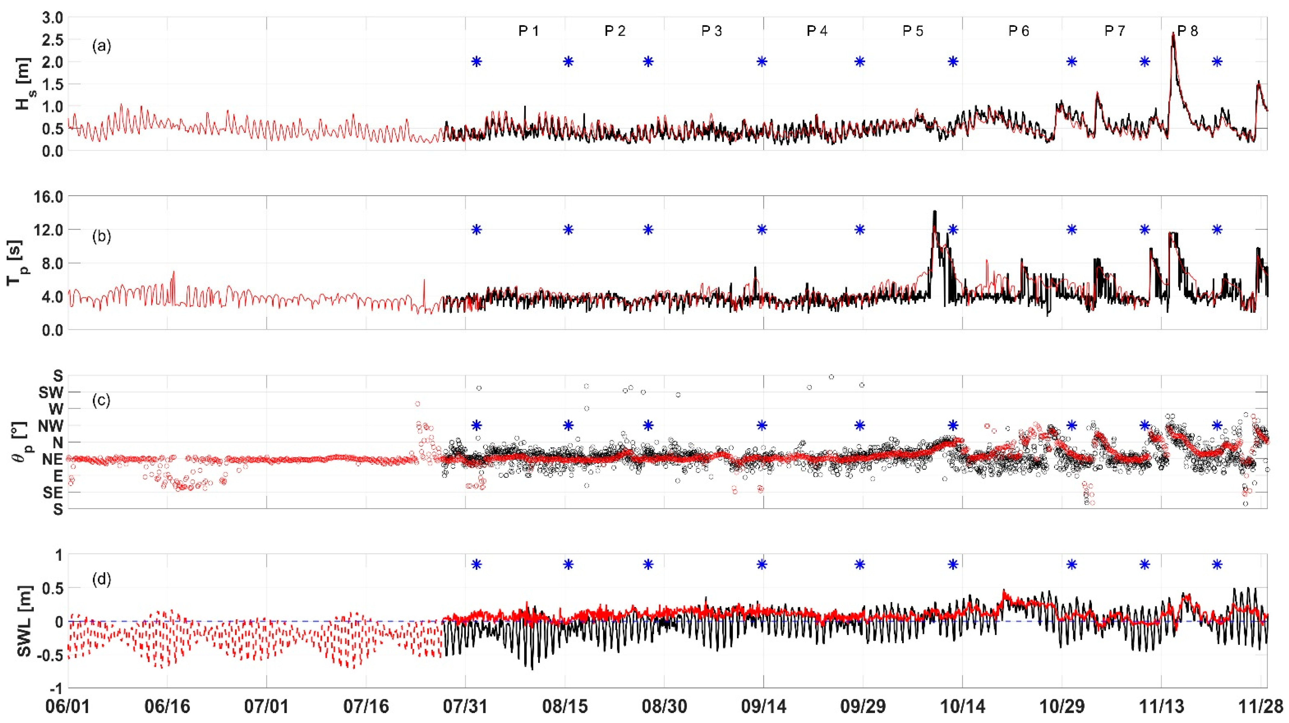
3.1. Description of Wave Conditions

To investigate the relationship between the spit evolution and the wave conditions, mean wave conditions, cumulative wave energy flux, and cumulative LST for the eight periods (between each survey) at the breaking zone are shown in Table 1 for the entire length of each period (“EP” columns) and during overwash, i.e., when SWL was higher than the spit height (“OP”, grey columns). June (Table 1, first row) showed relatively high wave conditions, which decreased in the next three months (periods 1 to 4). From October to November (periods 5 to 8), wave heights are the largest. Wave direction in the breaking zone also varies, generally decreasing throughout the study period, which is associated with the increase in cold fronts coming from the NNW.
In 2018 there were three cold fronts and two stationary fronts in November. The strongest cold front occurred on November 14 with waves coming from the NW–NE reaching heights of 2.8 m with peak periods of 12 s at the ADCP instrument location (10 m depth). The stationary fronts produce waves with longer periods (TP > 8 s) and 0.7 > HS > 1.0 m. October showed an atypical 72 h event with waves coming from the north, TP > 15 s, and Hs < 1 m, which was a possible consequence of hurricane Michael crossing the Yucatan Strait and traveling northwards into the Gulf of Mexico (7–12 October). A stationary front was located in the Gulf of Mexico from 16 to 25 October, and then it became the first cold front of the season, reaching the Yucatan shore on 29 October.

3.2. Qualitative Description of the Sand Spit in Its Early Stages

The spit formation was also captured with a video monitoring system. Due to the camera orientation and elements obstructing the view, these images are only used to qualitatively describe the initial morphological behavior (20 June to 31 July).
The spit was initially observed above MSL on 20 June 2018, approximately 15 m onshore from the east breakwater tip, as shown in Figure 4a. The previous month showed dominant westward sediment transport with waves coming predominantly from the NE (Table 1) producing saturation of the east breakwater. The consolidation period (1–13 July) was characterized by a notorious growth of the sand structure (Figure 4b). This was the least energetic period of the whole study and had the highest wave angle. On 14 July, Tropical Storm 15 produced energetic waves (HS ~0.82 m) that moved the spit onshore, especially the part attached to the breakwater (Figure 4c). Subsequently, on 19 July, another spit appeared (Figure 4d), although a submerged structure was already observed in the aftermath of the storm. The distance between the crests of these two spits was small, but it took almost two more weeks for them to merge (Figure 4e).

3.3. Seabreeze-Dominated Period

The UAV high-resolution surveys started on the first of August 2018 (Figure 3). The morphological characteristics (Table 1) were derived from digital elevation models (Figure 5). In the first survey, the spit had an average width of 5 m and was rounded at the tip; the structure reached 55 m in length and 20 cm above MSL with an area of 596 m2 and a volume of 135 m3.
The digital model of 15 August exhibits two sand bodies separated by ~50 m. The drone mosaic (Figure 3) suggests that the most offshore body was newly formed and the original structure migrated onshore. The digital model could not capture this because a large part of the original structure was submerged. By extracting a profile that follows a path of the highest elevations of the surveys (Figure 6), it can be seen that the elevation of the original spit lowered, and the tip migrated onshore 15 m. In addition, the base of the new spit was located further onshore than the base of the original one. By August 27, the new spit gained length and height and had a shape strikingly similar to the original spit. Moreover, the whole original spit was underwater at this point and remained undetected by the digital elevation model. This remnant roughly maintained its position and was gradually absorbed by the new spit by 28 September.
In Figure 7, we present a summary of the geometric characteristics of the spit and the daily rates of change per period. The gradual absorption (merging) of the two spits was manifested by a fast growth in length of the new spit (from 27 August to 28 September in Figure 7). In addition, the maximum spit height increased from 0.37 m to 0.51 m. This process occurred during the least energetic periods of the study (periods 2 and 3; see Table 1). During period 5 (between 28 September and 12 October), the area, width, and height grew, while the length remained constant. We consider this as a period of consolidation of the spit. Interestingly, this was the period with more wave energy before the nortes started.

3.4. Extreme Event Period or Norte Season

Generally, Central American cold surges (CACSs) arrive on the Northwestern side of the Yucatan Peninsula (locally known as nortes) from November to February. However, these events can also occur outside this period.
A stationary front was observed in the Gulf of Mexico by the end of October (period 6). As a result, the spit gained considerable amounts of sand, with a 70% growth in volume, 28% growth in area, 25% growth in length, and maximum height of 0.75 m. During this period, the cumulative longitudinal wave-energy flux reached its maximum (to the east, see Table 1).
The first cold front arrived on the peninsula on the second of November (period 7). This period was characterized by a similar wave height and period as the previous two, indicating that the cold front was mild. As a result, the spit grew in length and volume but maintained its maximum height given that no significant wave runup or storm surge occurred. Moreover, part of the sediment was redistributed towards the tip.
The most energetic cold front arrived on 14 November and lasted over 48 h, after which the spit was breached. This event exhibited the largest wave heights of the whole study period, reaching 2.5 m. In addition, this was the only period that had the dominant longitudinal wave flux with an opposite direction. In consequence, the area and volume were reduced by 45% and 75%, respectively. The spit elevation was reduced by 30%, reaching a maximum height of 0.51 m.

4. Discussion

4.1. Main Drivers of Spit Morphology

In recent years, there has been a surge in the use of UAVs to measure dynamic structures. Their main advantage is the high spatial and temporal resolution that can be achieved efficiently. Obtaining a topography over an area of 0.25 km2 with a UAV can be completed in less than an hour (considering GCP mandatory acquisition). The orthomosaic is another important output from UAVs (Figure 3). The shallow and clear waters of Yucatan allow observation of submerged sand structures, as well as vegetation and debris, that are not captured by the DEM. The combination of DEMs and the orthomosaic allows the analysis of complex morphological changes (e.g., sand spit merging). In this study, the observed spit behavior can be classified into (a) formation, (b) growth, (c) migration, (d) multiple spit interactions (merging), and (e) breaching.
(a)
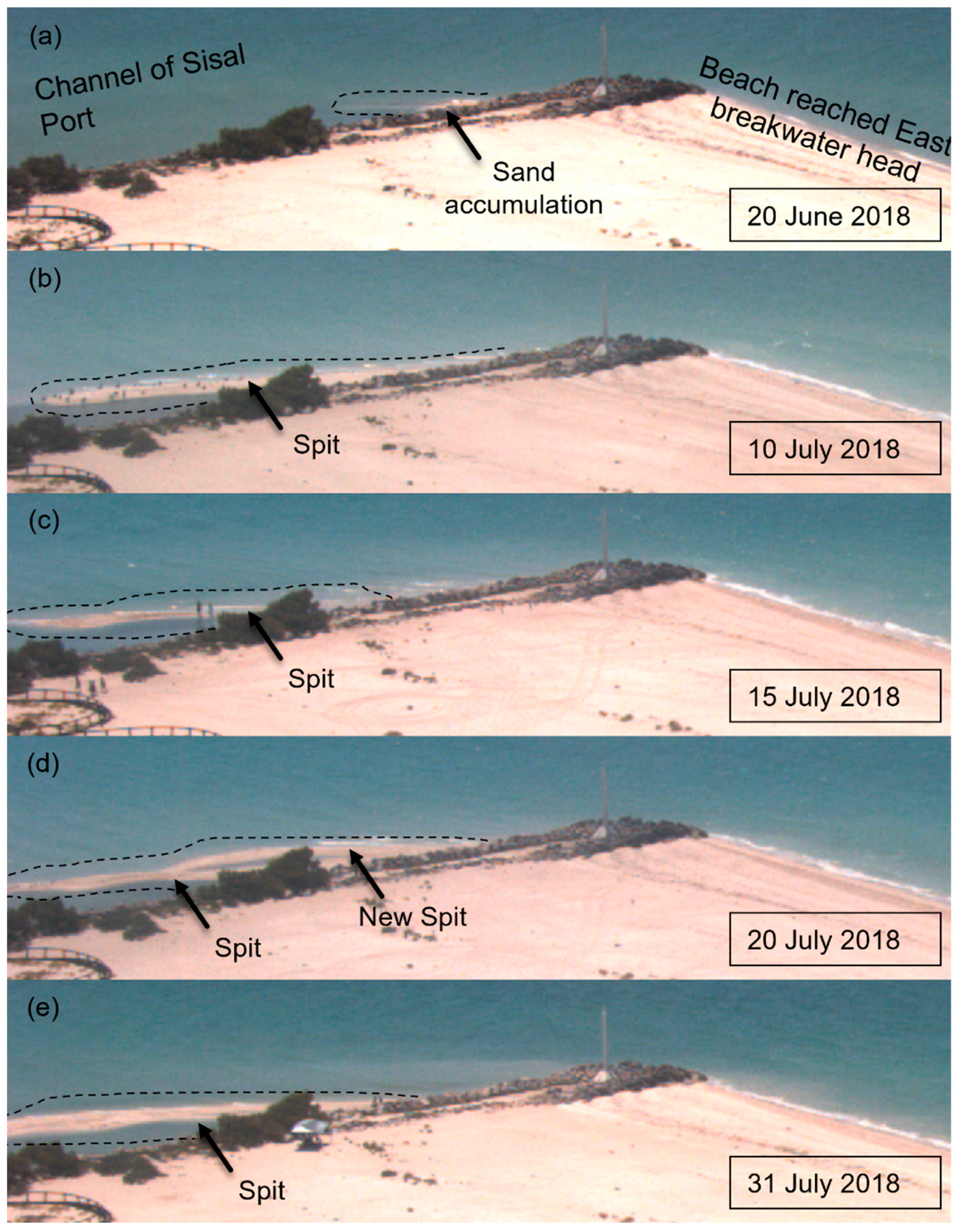
Formation: The formation conditions are shown in Table 1. The east breakwater of the port of Sisal imposes a discontinuity in the coastline which retains sediments, particularly from March to November (outside the norte season) when NE sea breeze waves dominate. Once the eastern breakwater was saturated (i.e., the eastern beach reached its tip) on 17 June, the magnitude of the littoral transport deposited in the port’s navigation channel increased and rapidly formed a coherent sand structure.
(b)
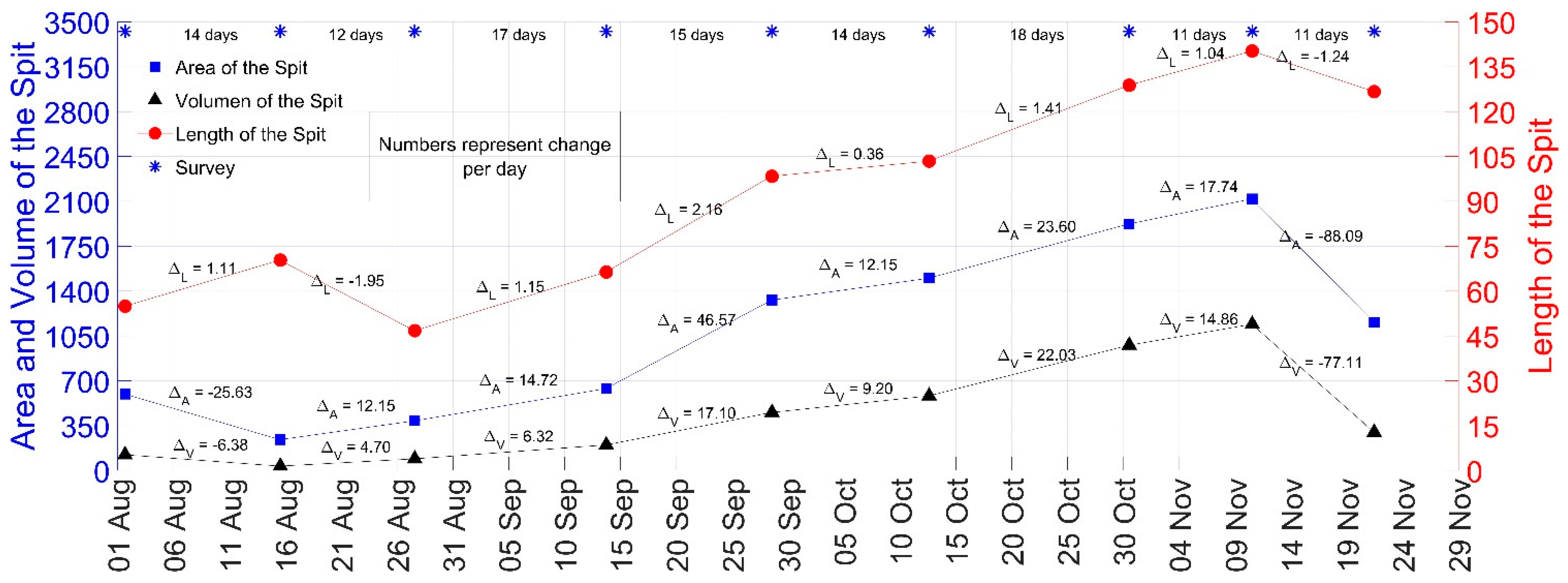
Growth: The spit grew in length and width under different conditions. The spit elongated faster with larger LST rates, responding to waves coming from ENE/NE. This occurred because the littoral transport fed the spit, and the breakwater reduced the energy of waves that could produce diffusion. The width increased with longer wave periods under moderate wave energy because a moderate increment in runup had the capacity to transport sand to the spit top. Furthermore, the morphological response of the spit not only depended on waves but also on the previous morphological state (e.g., if the spit is starting to form, or if it is consolidated). Some aspects that help us to determine the spit resistance are spit elevation and width. For example, the first cold front (5 November 2018) did not damage the structure. On the contrary, the spit grew in length and width, mainly because the previous morphological state of the spit was consolidated (spit height over 0.65 m), meaning that the energy threshold to breach the spit needed to be higher (HS > 1.2 m).
(c)
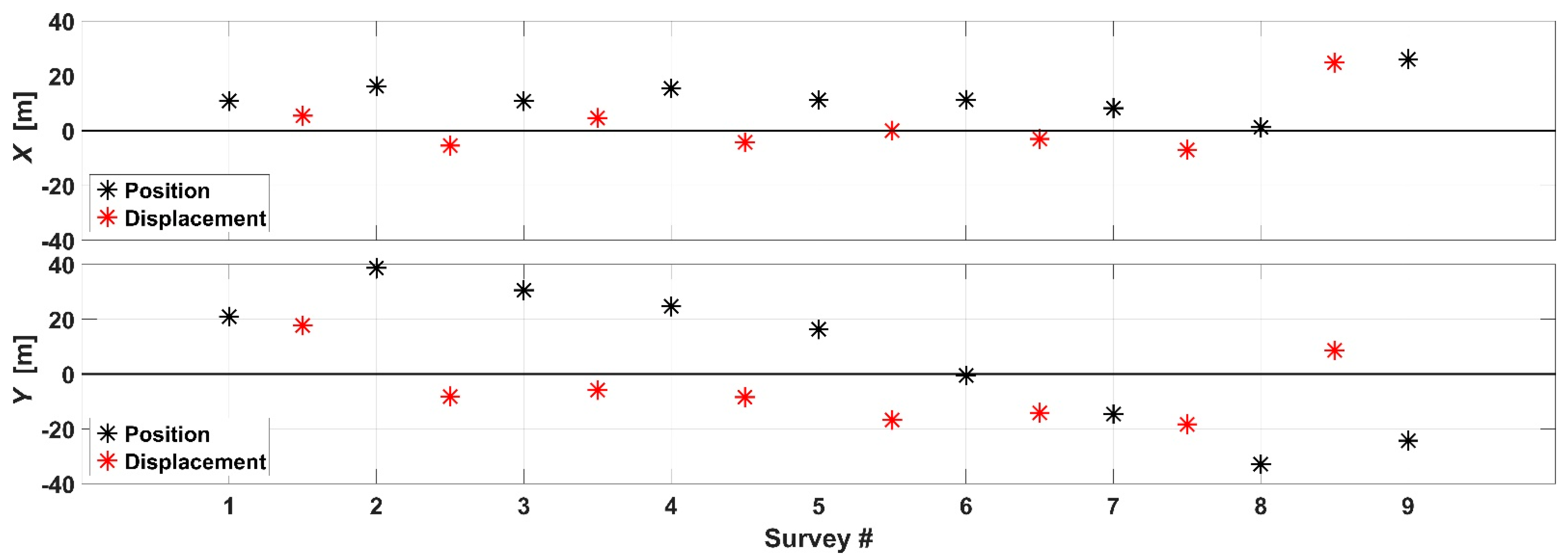
Migration: Figure 8 shows the position and displacement of the spit throughout the study. Displacements in X are small (less than 10 m) except after a breaching/destruction event. The relatively stable X position throughout the study period suggests that the input sediment is well distributed along the spit. The Y displacement is mostly onshore and is related to overwash events during high tide. The largest onshore migrations (periods 5 to 7) are related to an inversion in the direction of the longshore wave energy and a slight increase in the wave height magnitude (see Table 1, grey columns, where wave conditions were calculated for when the spit was below the MSL, i.e., during overwash). During destruction events, the apparent migration is offshore; is due to spit breaching, with the tip of the spit being detached and eroded by the waves (moving the sediment below sea level) and the attached zone of the spit retaining more sediment due to the protection provided by the breakwater, which causes the center of mass to move northeast.
(d)
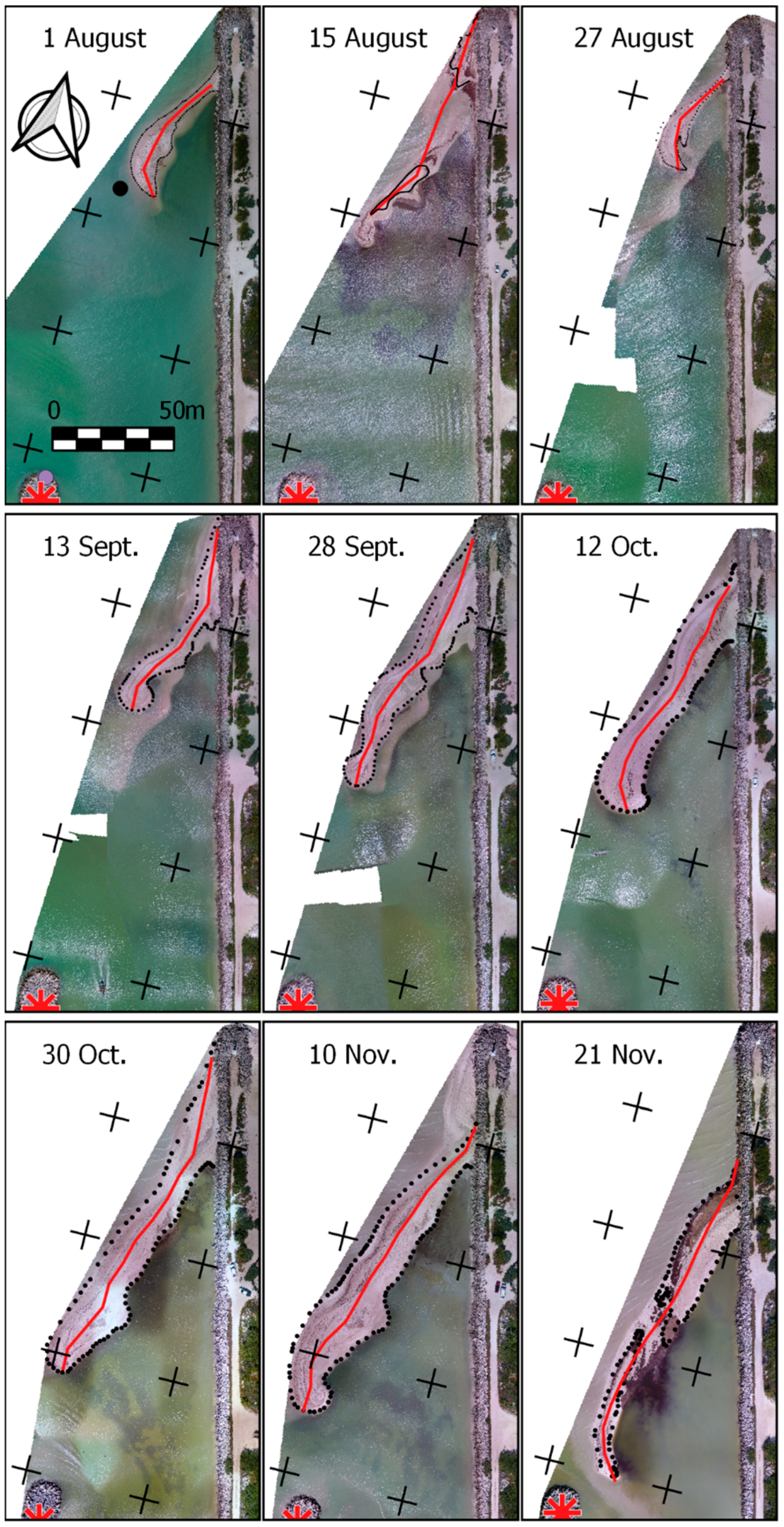
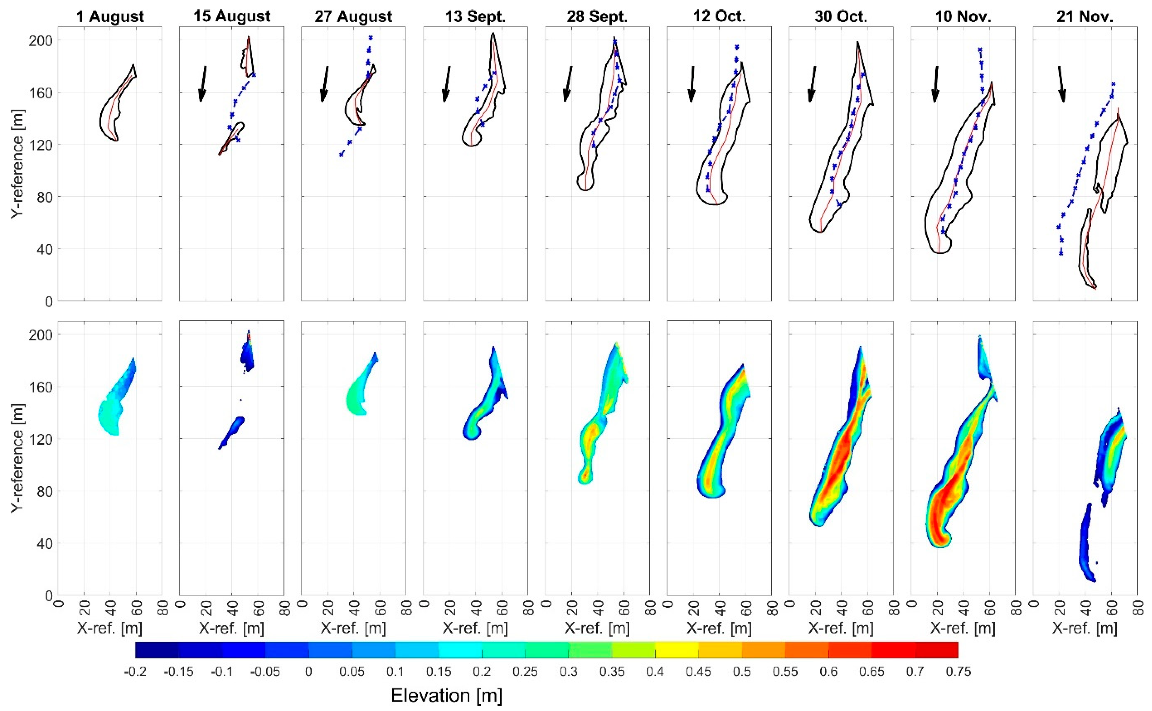
Multiple spit interactions (merging): The formation of a second spit can first be observed in the orthomosaic of 15 August, and two spits can be seen until 28 September (Figure 3). The next survey (27 August) shows that the older spit migrated onshore and the new spit grew. The first spit cannot be detected by the DEM because it is underwater. After 27 August, its position remains stable, while the second spit migrates gradually onshore. This occurs because the new spit absorbs the wave energy, protecting the spit vestige. The growth rate of the spit is accelerated by a merging process until the merging is completed on 12 October.
(e)
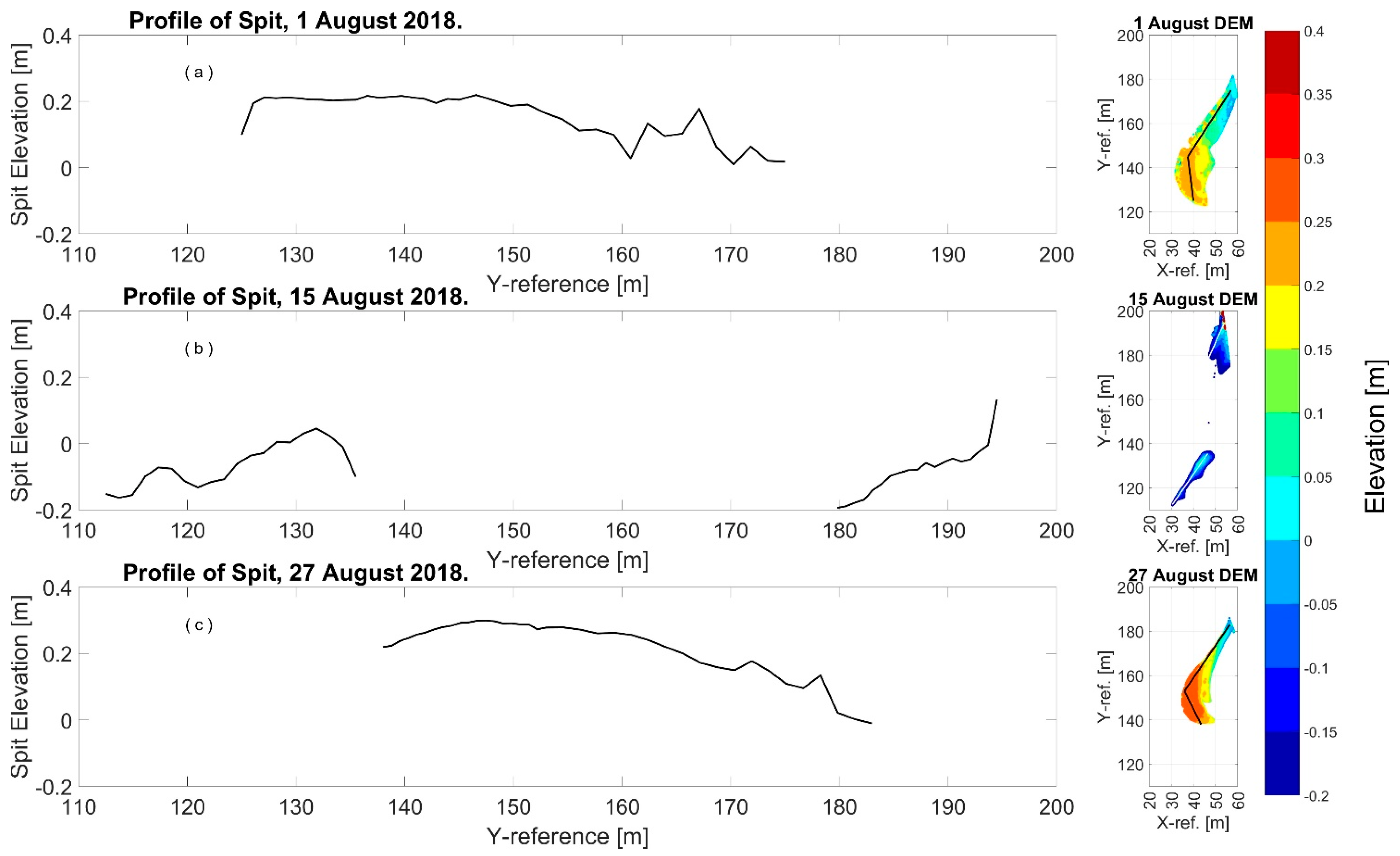
Breaching: Breaching is the result of the increase in wave energy and the sea level surge during nortes (see period 8 in Table 1). The mean wave height in the break zone was 0.88 m, with a corresponding direction of Db ~−7.35°. From Table 1 (grey columns) we observe that the time during which the spit is submerged in this period is 66% (i.e., 7.21 out of 10.92 days). Main changes are observed in the center of the spit, where a breach occurs (Figure 5). Maximum height is observed near the sheltered region (east jetty), while the center of the spit was below our measurement range, and at the same moment over 50% of the total area measured was near our lowest elevation (Z ~−0.20 m).
In addition to the above, recent studies [44,45,46,47] have suggested that infragravity waves (IGs) can have an impact on cross-shore sediment transport and therefore on the morphodynamics of inlets, mainly during storm conditions. In our study, storm conditions were present between surveys 6 and 9, generating significant cross-shore wave flux energy (Table 1, grey columns), especially when the spit was covered by water (MSL > highest spit elevation), producing 20 and 40 m displacements of the spit (Figure 8, surveys 7 and 8). Unfortunately, our instrument sampling setup did not resolve for IGs. However, to the best of our knowledge, the only recent study performed in a microtidal environment [47] reports that the IG wave energy represented only 4% of the maximum offshore storm energy, which might suggest that the impact of IGs may be small when the tidal amplitude and currents are small (microtidal coast), as is the case in our study site. In any case, a more in-depth study is necessary to evaluate the relevance of infragravity waves on the morphodynamics in the mixed-energy microtidal environments of the northern YP coast.

4.2. Importance of Morphological Monitoring in the Yucatan Harbors/Inlets

Although spits can occur in high-current macrotidal environments [7,13], sand spits are common on the north coast of Yucatan because of the combination of (a) interruptions in the coastline (by port channels or natural inlets opened mainly by hurricanes), (b) the alongshore sediment transport being predominantly westward most of the year, and (c) weak tidal currents (in a microtidal environment). In this area, sand spits can have a detrimental effect on the coastal socio-ecological systems. In particular, they affect the economy of the 12 fisher towns when the channels close, the water quality of the lagoons due to an increase in residence times and eutrophication, and eco-tourism activities that often rely on the quasi-pristine conditions of these environments (e.g., La Carbonera lagoon 15 km west of Sisal).
Monitoring in other sites has shed light on the cyclic nature [13] and on the correlation between run-up and morphological changes of a spit (being negative when the run-up exceeds the crest of the tongue and positive with longer periods and lower wave heights) [23]. Escudero et al. (2019) [8] conducted a study for a period of 31 years on a sand spit located at a beach 330 km west of the port of Sisal, where the orientation breaks at almost a 90° angle. They also found that the spit retreats after a synoptic-scale event (e.g., nortes and hurricanes), and the spit grows in fair weather conditions.
In Sisal, we observe that the saturation of the jetty is a prerequisite for spit formation, which occurs during summer, together with mild wave conditions. In addition, once the spit is consolidated, even though typical winter storms can reverse the alongshore sediment transport direction, they do not have the strength to diffuse the sand structure and, on the contrary, can accelerate the blockage of the port entrance.
Beach/sand structure monitoring is arduous with traditional techniques due to the difficulty that fieldwork represents, from remote sites to massive land areas to cover by a small group of people, as well as dynamic changes in short periods of time that make it difficult for researchers to calculate migration speed and observe phenomena such as spit destruction [48,49]. In that sense, the monitoring of spit morphology through drone surveys allows for an easy and cost-effective operation and a better understanding of the morphodynamics, consequently allowing for effective and timely management [13,21,22,23].
Observing the spit evolution characteristics and the spit volume before the storm season, we can recommend three main actions: (a) performing timely preventive dredging operations targeting the sand accumulation in the dry beach east of the jetty, rather than corrective dredging when the closure of the channels are imminent [17]; (b) implementing sand bypass systems across the port channels [50,51]; and (c) redesigning the jetties to promote a more efficient bypass of the sand without mechanical systems. This would hinder the spit growth potential and allow the typical winter storms to overcome the spit and diffuse the accumulated sand.
Furthermore, given that the Sisal port geometry (the length and orientation of jetties and the depth of the entrance) is different from that of other Yucatan ports (e.g., Chelem), expanding the monitoring to these ports would allow us to understand the influence of port geometry on spit development and, therefore, improve port design and management.

5. Conclusions

The evolution of a sand spit in the entrance of Sisal’s port was characterized using UAV surveys. Simultaneous measurements of waves and sea level were used to identify the mechanisms that drive the growth, migration, merging, and breaching of the sand spit. In particular, wave direction and overwash events played an important role in the spit evolution. Initial spit formation takes place during calm conditions (e.g., periods dominated by sea breezes), and according to the energy threshold of high energetic events, this new spit will consolidate or breach. Migration of the spit is related to overwash events and changes in wave direction.
The Sisal port channel is restricted by two jetties (like many other small ports of Yucatan); due to constant westward high energy wave flux, sand accumulates on the east jetty (updrift), and when the accreting coastline reaches the jetty head, the sand accumulation extends to the port channel. Since there is no preventive coastal management plan, this process can lead to channel blockage. When a sand spit forms in the access channel and when high energetic events occur (e.g., storms or norte cold fronts), extreme wave conditions and higher water levels move the sand spit further into the channel and diffuse it, obstructing navigation and water flow circulation, thus generating socio-ecological problems; it is at this moment when dredging occurs.
Constant monitoring of the coast, including hydrodynamic measurements and UAV flights over the zone, is recommended to observe the development of morphological features in the fishing ports. For a community that relies on fisheries, a lot can be lost if a port channel is closed by a sand structure. Thus, highlighting the importance of frequent measurements and a dredging plan is essential for these communities and local governments.

Author Contributions

Conceptualization, P.S., J.L.-G. and A.P.-H. methodology, A.P.-H., P.S., J.L.-G. and J.A.; software, A.P.-H.; formal analysis, A.P.-H.; investigation, A.P.-H.; resources, P.S.; data curation, A.P.-H.; writing—original draft preparation, A.P.-H. and J.A.; writing—review and editing, P.S., A.P.-H., J.A. and J.L.-G.; visualization, A.P.-H.; supervision, P.S.; project administration, P.S., J.L.-G. and J.A.; funding acquisition, P.S. All authors have read and agreed to the published version of the manuscript.

Funding

This research was funded by CONACyT-SENER with a PhD scholarship to Alejandro Paladio Hernandez with CVU 511266, as well as project PAPIIT-UNAM 111916.

Institutional Review Board Statement

Not applicable.

Informed Consent Statement

Not applicable.

Data Availability Statement

The wind data presented are openly available in https://www.ruoa.unam.mx/ (accessed on 8 January 2019). Wave data from Wavewatch III are openly available in https://polar.ncep.noaa.gov/ accessed on 23 September 2019. The data presented in this study are available on request from the corresponding author.

Acknowledgments

We acknowledge the Engineering Institute (Sisal Unit) of UNAM and the National Coastal Resilience Laboratory for providing the necessary equipment for measurements. In addition, we would like to thank Gonzalo Uriel Martin (IT Support) and Juan Alberto Gomez Liera (fieldwork support).

Conflicts of Interest

The authors declare no conflict of interest.

References

  1. Cowell, P.J.; Thom, B.G.; van de Plassche, O. Morphodynamics of coastal evolution. In Coastal Evolution: Late Quaternary Shoreline Morphodynamics; Carter, R.W.G., Woodroffe, C.D.E., Eds.; Cambridge University Press: Cambridge, UK, 1995; pp. 33–86. [Google Scholar]
  2. Coco, G.; Murray, A.B. Patterns in the sand: From forcing templates to self-organization. Geomorphology 2007, 91, 271–290. [Google Scholar] [CrossRef]
  3. Kraus, N.C.; ASCE, M. Analytical Model of Spit Evolution at Inlets. Proc. Coast. Sediments 1999, 3, 1739–1754. [Google Scholar]
  4. Serizawa, M.; Uda, T.; Miyahara, S. Prediction of Formation of Recurved Sand Spit Using Bg Model. Coast. Eng. Proc. 2019, 1, 24. [Google Scholar] [CrossRef] [Green Version]
  5. Riggs, S.R.; Cleary, W.J.; Snyder, S.W. Influence of inherited geologic framework on barrier shoreface morphology and dynamics. Mar. Geol. 1995, 126, 213–234. [Google Scholar] [CrossRef]
  6. Evans, O.F. The Origin of Spits, Bars, and Related Structures. J. Geol. 1942, 50, 846–865. [Google Scholar] [CrossRef]
  7. Allard, J.; Bertin, X.; Chaumillon, E.; Pouget, F. Sand spit rhythmic development: A potential record of wave climate variations? Arçay Spit, western coast of France. Mar. Geol. 2008, 253, 107–131. [Google Scholar] [CrossRef]
  8. Escudero, M.; Silva, R.; Hesp, P.A.; Mendoza, E. Morphological evolution of the sandspit at Tortugueros Beach, Mexico. Mar. Geol. 2019, 407, 16–31. [Google Scholar] [CrossRef]
  9. Murray, A.B.; Ashton, A.; Arnoult, O. Large-scale morphodynamic consequences of an instability in alongshore transport. In Proceedings of the 2nd IAHR Symposium on River, Coastal and Estuarine Morphodynamics, Obihiro, Japan, 10–14 September 2001; pp. 355–364. [Google Scholar]
  10. Ashton, A.D.; Murray, A.B. High-angle wave instability and emergent shoreline shapes: 2. Wave climate analysis and comparisons to nature. J. Geophys. Res. Earth Surf. 2006, 111, F04012. [Google Scholar] [CrossRef] [Green Version]
  11. Ashton, A.D.; Murray, A.B. High-angle wave instability and emergent shoreline shapes: 1. Modeling of sand waves, flying spits, and capes. J. Geophys. Res. Earth Surf. 2006, 111, F04011. [Google Scholar] [CrossRef] [Green Version]
  12. Fitzgerald, D.M.; Penland, S.; Nummedal, D. Control of Barrier Island Shape by Inlet Sediment Bypassing: East Frisian Islands, West Germany. Mar. Geol. 1984, 60, 355–376. [Google Scholar] [CrossRef]
  13. Robin, N.; Levoy, F.; Anthony, E.J.; Monfort, O.; France, C. Sand spit dynamics in a large tidal-range environment: Insight from multiple LiDAR, UAV and hydrodynamic measurements on multiple spit hook development, breaching, reconstruction, and shoreline changes. Earth Surf. Process. Landf. 2020, 45, 2706–2726. [Google Scholar] [CrossRef]
  14. Inman, D.L.; Dolan, R. The Outer Banks of North Carolina: Budget of Sediment and Inlet Dynamics along a Migrating Barrier System. J. Coast. Res. 1989, 5, 193–237. [Google Scholar]
  15. Talavera, L.; Río, L.D.; Benavente, J.; Barbero, L.; López-Ramírez, J.A. UAS & SfM-based approach to Monitor Overwash Dynamics and Beach Evolution in a Sandy Spit. J. Coast. Res. 2018, 85, 221–225. [Google Scholar]
  16. Talavera, L.; Del Río, L.; Benavente, J. UAS-based High-resolution Record of the Response of a Seminatural Sandy Spit to a Severe Storm. J. Coast. Res. 2020, 95, 679–683. [Google Scholar] [CrossRef]
  17. Wiegel, R.L. Sand Bypassing at Santa Barbara, California. J. Waterw. Harb. Div. 1959, 85, 1–30. [Google Scholar] [CrossRef]
  18. Komar, P.D.; Moore, J.R. CRC Handbook of Coastal Processes and Erosion; CRC Press: Boca Raton, FL, USA, 1983. [Google Scholar]
  19. Ogawa, Y.; Fujita, Y.; Shuto, N. Change in the Cross-Sectional Area and Topography At River Mouth. Coast. Eng. Japan 1984, 27, 233–247. [Google Scholar] [CrossRef]
  20. Tanaka, H.; Takahashi, F.; Takahashi, A. Complete Closure of The Nanakita River Mouth in 1994. Coast. Eng. 1996, 4545–4556. [Google Scholar]
  21. Casella, E.; Rovere, A.; Pedroncini, A.; Stark, C.P.; Casella, M.; Ferrari, M.; Firpo, M. Drones as tools for monitoring beach topography changes in the Ligurian Sea (NW Mediterranean). Geo-Mar. Lett. 2016, 36, 151–163. [Google Scholar] [CrossRef]
  22. Duy, D.V.; Tanaka, H.; Mitobe, Y.; Anh, N.Q.D.; Viet, N.T. Sand Spit Elongation and Sediment Balance at Cua Lo Inlet in Central Vietnam. J. Coast. Res. 2018, 81, 32. [Google Scholar]
  23. Sasaki, Y.; Sato, S. Morphology Changes of Sand Spit Around the Tenryu River Mouth Due To Floods Accompanied with Overtopping Waves. In Coastal Sediments 2015; World Scientific Publishing Co.: Toh Tuck Link, Singapore, 2015; pp. 1–14. [Google Scholar]
  24. Long, N.; Millescamps, B.; Guillot, B.; Pouget, F.; Bertin, X. Monitoring the topography of a dynamic tidal inlet using UAV imagery. Remote Sens. 2016, 8, 387. [Google Scholar] [CrossRef] [Green Version]
  25. Franklin, G.L.; Medellín, G.; Appendini, C.M.; Gómez, J.A.; Torres-Freyermuth, A.; López González, J.; Ruiz-Salcines, P. Impact of port development on the northern Yucatan Peninsula coastline. Reg. Stud. Mar. Sci. 2021, 45, 101835. [Google Scholar] [CrossRef]
  26. Enriquez, C.; Mariño-Tapia, I.J.; Herrera-Silveira, J.A. Dispersion in the Yucatan coastal zone: Implications for red tide events. Cont. Shelf Res. 2010, 30, 127–137. [Google Scholar] [CrossRef]
  27. Appendini, C.M.; Salles, P.; Tonatiuh Mendoza, E.; López, J.; Torres-Freyermuth, A. Longshore Sediment Transport on the Northern Coast of the Yucatan Peninsula. J. Coast. Res. 2012, 28, 1404–1417. [Google Scholar] [CrossRef]
  28. Torres-Freyermuth, A.; Puleo, J.A.; DiCosmo, N.; Allende-Arandía, M.E.; Chardón-Maldonado, P.; López, J.; Figueroa-Espinoza, B.; de Alegria-Arzaburu, A.R.; Figlus, J.; Roberts Briggs, T.M.; et al. Nearshore circulation on a sea breeze dominated beach during intense wind events. Cont. Shelf Res. 2017, 151, 40–52. [Google Scholar] [CrossRef]
  29. Tenorio-Fernandez, L.; Gomez-Valdes, J.; Marino-Tapia, I.; Enriquez, C.; Valle-Levinson, A.; Parra, S.M. Tidal dynamics in a frictionally dominated tropical lagoon. Cont. Shelf Res. 2016, 114, 16–28. [Google Scholar] [CrossRef]
  30. Pacheco-Castro, R.; Salles, P.; Canul-Macario, C.; Paladio-Hernandez, A. On the understanding of the hydrodynamics and the causes of saltwater intrusion on lagoon tidal springs. Water 2021, 13, 3431. [Google Scholar] [CrossRef]
  31. Santoyo Palacios, B.A. Technical Report: Esbozo Monográfico de Sisal, Yucatán; LANRESC: Yucatán, México, 2017. [Google Scholar]
  32. Wellmann, N. Analysis of Near-Shore Sediment Samples from Sisal Beach (Mexico) Comparing Effects of Sea Breeze and el Norte Events. Ph.D. Thesis, Wirtschaft und Kultur Leipzig, Stuttgart, Germany, 2014. [Google Scholar]
  33. Medellín, G.; Torres-Freyermuth, A. Morphodynamics along a micro-tidal sea breeze dominated beach in the vicinity of coastal structures. Mar. Geol. 2019, 417, 106013. [Google Scholar] [CrossRef]
  34. Medellín, G.; Torres-Freyermuth, A.; Tomasicchio, G.R.; Francone, A.; Tereszkiewicz, P.A.; Lusito, L.; Palemón-Arcos, L.; López, J. Field and numerical study of resistance and resilience on a sea breeze dominated beach in Yucatan (Mexico). Water 2018, 10, 1806. [Google Scholar] [CrossRef] [Green Version]
  35. Zavala-Hidalgo, J.; de Buen Kalman, R.; Romero-Centeno, R.; Hernández Maguey, F. Tendencias del nivel del mar en las costas mexicanas. Vulnerabilidad las Zonas Costeras Mexicanas Ante el Cambio Climático; Semarnat-INE, UNAM-ICMyL, Universidad Autónoma de Campeche: Campeche, México, 2010; pp. 249–267. [Google Scholar]
  36. Zavala-Hidalgo, J.; Morey, S.L.; O’Brien, J.J. Seasonal circulation on the western shelf of the Gulf of Mexico using a high-resolution numerical model. J. Geophys. Res. 2003, 108, 3389. [Google Scholar] [CrossRef]
  37. Modesto, O.F.; Ernesto, A.V. Software MARV 1.0. 2015. Tidal Prediction in Mexico. Available online: http://predmar.cicese.mx/ (accessed on 15 August 2020).
  38. Figueroa-Espinoza, B.; Salles, P.; Zavala-Hidalgo, J. On the wind power potential in the northwest of the Yucatan Peninsula in Mexico. Atmosfera 2014, 27, 77–89. [Google Scholar] [CrossRef] [Green Version]
  39. Kurczyn, J.A.; Appendini, C.M.; Beier, E.; Sosa-López, A.; López-González, J.; Posada-Vanegas, G. Oceanic and atmospheric impact of central American cold surges (Nortes) in the Gulf of Mexico. Int. J. Climatol. 2020, 41, E1450–E1468. [Google Scholar] [CrossRef]
  40. Lopez-Gonzalez, J.; Dominguez Sandoval, M.F. Caracterizacion de oleaje frente a la costa de Sisal Yucatán. In Caracterización Multidisciplinaria de la Zona Costera de Sisal, Yucatán; Laboratorio Nacional de Resiliencia Costera: Hunucmá, Mexico, 2017; pp. 30–39. [Google Scholar]
  41. Torres-Freyermuth, A.; Medellín, G.; Mendoza, E.T.; Ojeda, E.; Salles, P. Morphodynamic response to low-crested detached breakwaters on a sea breeze-dominated coast. Water 2019, 11, 635. [Google Scholar] [CrossRef] [Green Version]
  42. United States. Army Corps of Engineers, Coastal Engineering Manual—Part III. Coast. Eng. Man. 2008, EM 1100-2-1100, 1–62. [Google Scholar]
  43. Pix4D. Software: Pix4Dmapper. 2017. Available online: https://www.pix4d.com/download-software (accessed on 4 December 2018).
  44. Bertin, X.; de Bakker, A.; van Dongeren, A.; Coco, G.; André, G.; Ardhuin, F.; Bonneton, P.; Bouchette, F.; Castelle, B.; Crawford, W.C.; et al. Infragravity waves: From driving mechanisms to impacts. Earth-Sci. Rev. 2018, 177, 774–799. [Google Scholar] [CrossRef] [Green Version]
  45. Bertin, X.; Mendes, D.; Martins, K.; Fortunato, A.B.; Lavaud, L. The Closure of a Shallow Tidal Inlet Promoted by Infragravity Waves. Geophys. Res. Lett. 2019, 46, 6804–6810. [Google Scholar] [CrossRef]
  46. Mendes, D.; Fortunato, A.B.; Bertin, X.; Martins, K.; Lavaud, L.; Nobre Silva, A.; Pires-Silva, A.A.; Coulombier, T.; Pinto, J.P. Importance of infragravity waves in a wave-dominated inlet under storm conditions. Cont. Shelf Res. 2020, 192, 104026. [Google Scholar] [CrossRef]
  47. Melito, L.; Postacchini, M.; Sheremet, A.; Calantoni, J.; Zitti, G.; Darvini, G.; Penna, P.; Brocchini, M. Hydrodynamics at a microtidal inlet: Analysis of propagation of the main wave components. Estuar. Coast. Shelf Sci. 2020, 235, 106603. [Google Scholar] [CrossRef]
  48. Donnelly, C.; Kraus, N.; Larson, M. State of knowledge on measurement and modeling of coastal overwash. J. Coast. Res. 2006, 22, 965–991. [Google Scholar] [CrossRef]
  49. Parnell, K.E.; Hosking, P.L.; McLean, R.F.; Nichol, S.L. Multidecadal Shoreline Monitoring at Parengarenga, Northern New Zealand: From Dumpy Level to LiDAR. J. Coast. Res. 2020, 101, 165. [Google Scholar] [CrossRef]
  50. Callaghan, D.; Nielsen, P.; Zyserman, J.A.; Braker, I. Morphological Model for a Fixed Sand Bypass System. In Coastal Engineering 2002: Solving Coastal Conundrums, Proceedings of the 28th International Conference, Cardiff, UK, 7–12 July 2002; World Scientific Pub. Co.: Singapore, 2003; pp. 3845–3857. [Google Scholar]
  51. Murray, R.J.; Brodie, R.P.J.; Porter, M.; Robinson, D.A. Tweed River Sand Bypass: Concepts and Progress. In Coastal Engineering 1996; ASCE: Reston, VA, USA, 1996; pp. 4390–4396. [Google Scholar]
Figure 1. Study site location maps. (a) Global location; (b) Gulf of Mexico and the Yucatan Peninsula; red star marks the study site area in (a,b); (c) Sisal port (nearly 95,000 m2), Sisal community (orange polygon); the red circle is the camera system tower location and the black triangle is the position of the anemometer; the red lines are (from west to east) West Jetty, East Jetty, and Sisal Pier; the black line represents the coastline (sea to the north, wetlands to the south of the barrier island); (d) wind speed rose; (e) wave height rose (ADCP location is 10 km offshore of Sisal at 21°16.475′ N, −90°3.045′ W).
Jmse 10 00600 g001
Figure 2. ADCP wave and tidal conditions. Offshore significant wave height (a), peak wave period (b), peak wave angle (c), and surface water level (d) during the study. For panels (ac), red continuous lines are WaveWatch III data, and black lines are measured data. The blue stars correspond to the survey dates, and the numbers correspond to each “period” analyzed. In panel (d), the astronomical tide is shown from June to the end of July; the black continuous line (August to November) is the measured SWL, and the red continuous line is the residual tide (=SWL − astronomical tide).
Jmse 10 00600 g002
Figure 3. UAV images showing the evolution of the sand spit. The numbers are month/day of 2018. The red asterisk is the reference point. Crosses in each panel are 50 m apart in XY direction. The red lines show the center (midline) of the spit, and the black dotted lines correspond to the elevation Z = −0.2 m. The black dot in the first panel is a reference point used to compute the spit position and displacement.
Jmse 10 00600 g003
Figure 4. Array of snapshot images from the video monitoring system (location in Figure 1c) from June and July, when the spit was first recorded (a), maximum length reached before overwash event (b), during overwash event (c), after overwash (d), and merging after overwash (e). Spit is shown inside the black dashed line.
Jmse 10 00600 g004
Figure 5. Spit evolution throughout the study. Upper panels: contours (black line) and center of the spit (red line); starting on 15 August, each upper panel presents the centerline of the previous spit (blue dashed line). Wave direction between surveys is shown with a black arrow next to the spit. Lower panels: spit elevation, used for the volume calculation. XY values are in meters, measured from the west jetty head (red star in Figure 3).
Jmse 10 00600 g005
Figure 6. Spit profiles from (a) 1 August, (b) 15 August, and (c) 27 August, showing the spit before breaching, the breached spit, and the new spit profile, respectively. Right column panels show the digital elevation model, and the black lines (or white in the middle panel) are where the profiles (left panels) were computed.
Jmse 10 00600 g006
Figure 7. Computed length (m), area (m2), and volume (m3) during the eight periods of the study. ΔL (m/day), ΔA (m2/day), and ΔV (m3/day) represent the daily rate of change during each period.
Jmse 10 00600 g007
Figure 8. Position (black stars) of spit center of mass with respect to first survey minimum XY values, and displacement (red stars), which is the difference between each survey position. The position calculations were performed using accumulated weighted elevation (see Section 2.2) with X (upper panel) and Y (lower panel) coordinates. Black stars (position) show where the highest center of mass moves with respect to the first spit. Positive values represent east (in X) and north (in Y). For example, in the second survey, the spit center of mass moves to the east (positive X value in the upper panel) and to the north (positive Y value in the lower panel).
Jmse 10 00600 g008
Table 1. Duration (time elapsed between measurements), wave conditions (TPB and θWB are weighted averages, as a function of Hb), longshore and cross-shore components of wave flux, and cumulative sediment transport (using CERC formula).
PeriodEP a (Days)OP b (Days)Hb (m)TPB (s)θWB (°)CLWF c (103 W/m)CCWF d (103 W/m)CLST e (103 m3)Area (m2)Len. (m)Vol. (m3)
EPOP EPOP EPOP EPOP EPOP EPOP
f30.00 0.55 4.52 11.05 241.40 632.60 178.60
g31.58 0.410.413.693.6910.9510.95132.30132.30348.80348.8097.9097.9059655135
113.886.830.490.513.853.737.982.33178.9011.00662.40136.10132.408.202417034
212.087.500.370.373.533.538.312.4681.305.20286.0061.0060.103.903884791
317.0812.920.430.483.763.728.402.32171.109.70593.00119.00126.607.2063966199
414.829.750.420.503.623.4810.604.23187.308.00515.4054.30138.605.90132998453
514.058.790.620.636.244.613.46−1.11133.40−15.001138.60390.9098.70−11.101500103582
617.9512.040.660.644.374.218.41−2.14492.80−22.201741.00314.20364.70−16.401923129977
711.001.580.630.615.303.964.00−1.62139.90−0.301058.906.30103.60−0.3021181401141
810.927.210.880.939.536.70−7.35−11.3−954.70−500.463747.301294.60−706.60−370.401156127298
a Entire period. Values are calculated for the whole period. b Overwash period. Values are only calculated when SWL is higher than the maximum spit height. c Cumulative longitudinal wave flux. d Cumulative cross-shore wave flux. e Cumulative longshore sediment transport. f Spit was not surveyed, wave conditions correspond to June. g Spit was not surveyed, wave conditions correspond to July.
Publisher’s Note: MDPI stays neutral with regard to jurisdictional claims in published maps and institutional affiliations.

