Preventive Maintenance of a k-out-of-n System with Applications in Subsea Pipeline Monitoring

Abstract

Environmental safety issues are of particular importance when we design and operate underwater transport systems. To ensure the transport systems function safely, special systems to monitor their condition are being created. Underwater pipeline monitoring systems should continuously operate to detect and prevent emergency and pre-emergency situations in a timely manner. The purpose of this article is to demonstrate the possibility of using a mathematical model of a k-out-of-n system to support decision-making in the preventive maintenance of an unmanned underwater vehicle to monitor the condition of a subsea pipeline. The novelty and feature of this study are that we investigate a strategy of preventive maintenance for a model of a k-out-of-n system, where failures depend not only on the number but also on the location of the failed components in the system. The method to solve this problem, based on the distribution of the members of the variational series of the failing components, is also new. Since the distributions of the system component lifetimes are usually known with an accuracy of only one or two moments, we paid special attention to how sensitive the decision making about preventive maintenance is to the shape of the distributions. Numerical examples are conducted in order to support the theoretical investigations of the paper. The results of the study are applied to specific equipment to monitor the state of the outer surface of the pipeline.

1. Introduction, Motivation and an Example

1.1. Introduction

Environmental safety issues are one of the main problems of humanity in recent times. Currently, with industrial development and the new challenges that appear in connection with this, the issues of preventive environmental protection are gaining great importance. Work in the field of underwater transportation of hazardous products (such as oil, gas, etc.) draws special attention to these problems. In this regard, projects in the field of construction and operation of underwater oil or gas transportation systems should be accompanied by continuous monitoring of their condition. For such monitoring, special systems and equipment have been developed. However, this equipment is also susceptible to failures, and special preventive maintenance (PM) procedures must be provided to keep it in proper operational condition.

This work is devoted to the development of a mathematical model to organize such maintenance of pipeline transport underwater monitoring equipment based on the k-out-of-n model. The novelty and features of this study are that the point of failure of the system depends on where the system’s failing components are located, as well as in the study of the sensitivity of decision making on the type of distribution of their lifetime. This paper is to some extent related to the paper [1], also published in this issue, both of them focus on mathematical models that can contribute to safe, secure and sustainable pipeline transport offshore. However, this paper deals with another problem that can be solved with a k-out-of-n model—a reliability management problem—that is how to choose the best PM mode. So, we develop and investigate new methodology and provide an example of its real life application to subsea pipeline monitoring systems. Nevertheless, some parts of the introduction about k-out-of-n systems and the notations coincide with those in [1].

A k-out-of-n system is a system that contains n components in parallel and may be described in two ways, depending on the definition of the parameter k. The parameter k may represent the number of components in the system that must function for the entire system to work, referred to as a k-out-of-$n:G$ system. On the other hand, parameter k may represent the number of components in the system such that when the components fail, the entire system fails, referred to as a k-out-of-$n:F$ system [2]. Of course, these descriptions are closely connected and each of them is dual to another. Since for our aims it is more convenient to consider the subset of failed components of the system, in this paper we use the second type of system description.

Study of k-out-of-n systems reliability is interesting both from theoretical and practical points of view. From a theoretical point of view, it gives the wide possibility for new mathematical methods and applications. From a practical point of view, there are many investigations devoted to the reliability-centric analysis of k-out-of-n systems. The application of such models can be seen in many real-world phenomena, including telecommunication, transmission, transportation, manufacturing, and service applications. A probabilistic study of a real-world k-out-of-n system often helps to develop an optimal strategy to maintain high-level of system reliability. Thus, the theory of the k-out-of-n repairable systems is quite developed, but it does not cease to attract attention of researchers. Models are being developed taking into account various features of the systems. An important issue is to investigate the practical aspects of the application of these models. One of the applications of such kind of systems is described in the next subsection, where an automated system for remote monitoring of underwater sections of the “Dzhubga-Lazarevskoye-Sochi” gas pipeline is considered.

The paper is organized as follows. In the next subsection, an example of a real monitoring system, where we have to justify our choice of PM strategy, is presented. Further, this example will be used to demonstrate our theoretical research and proposed algorithms with the results of numerical calculations. A short literature review is given in Section 1.3. Section 2 contains the state of the problem and some notations. Section 3 presents general procedure of the PM quality calculation and gives an algorithm to solve the problem. Further, in Section 4, we consider the conditions to make PM efficient for the homogeneous system, where system failure does not depend on the failed components location. A model of PM organization for a system, where system failure depends on the location of its failed components is presented in Section 5. In the conclusion, further directions for research are proposed.

1.2. An Automated System for Remote Monitoring of Underwater Pipeline as an Example of k-out-of-n:F System

As an example of such kind of systems, we consider an automated system for remote monitoring of underwater sections of the “Dzhubga-Lazarevskoye -Sochi” gas pipeline [3]. The annual capacity of the pipeline is up to 3.78 billion cubic meters of gas. Estimated service life is 50 years. Total length is 171.6 km, where the offshore part of the gas pipeline accounts for some 90 per cent of the whole route length. The route runs some 4.5 km off the coast where the sea depth reaches 80 m. Linepipe diameter is 530 mm, wall thickness—15 mm for the offshore and 11.3 mm for the onshore part of the gas pipeline, material—high strength steel.

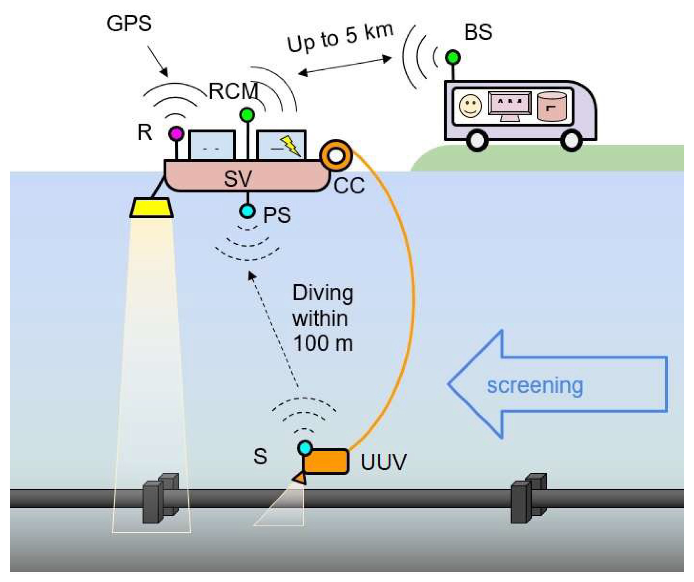
Figure 1 shows the general concept of an automated system to remotely inspect of the offshore section of the gas pipeline using an unmanned underwater vehicle (UUV).

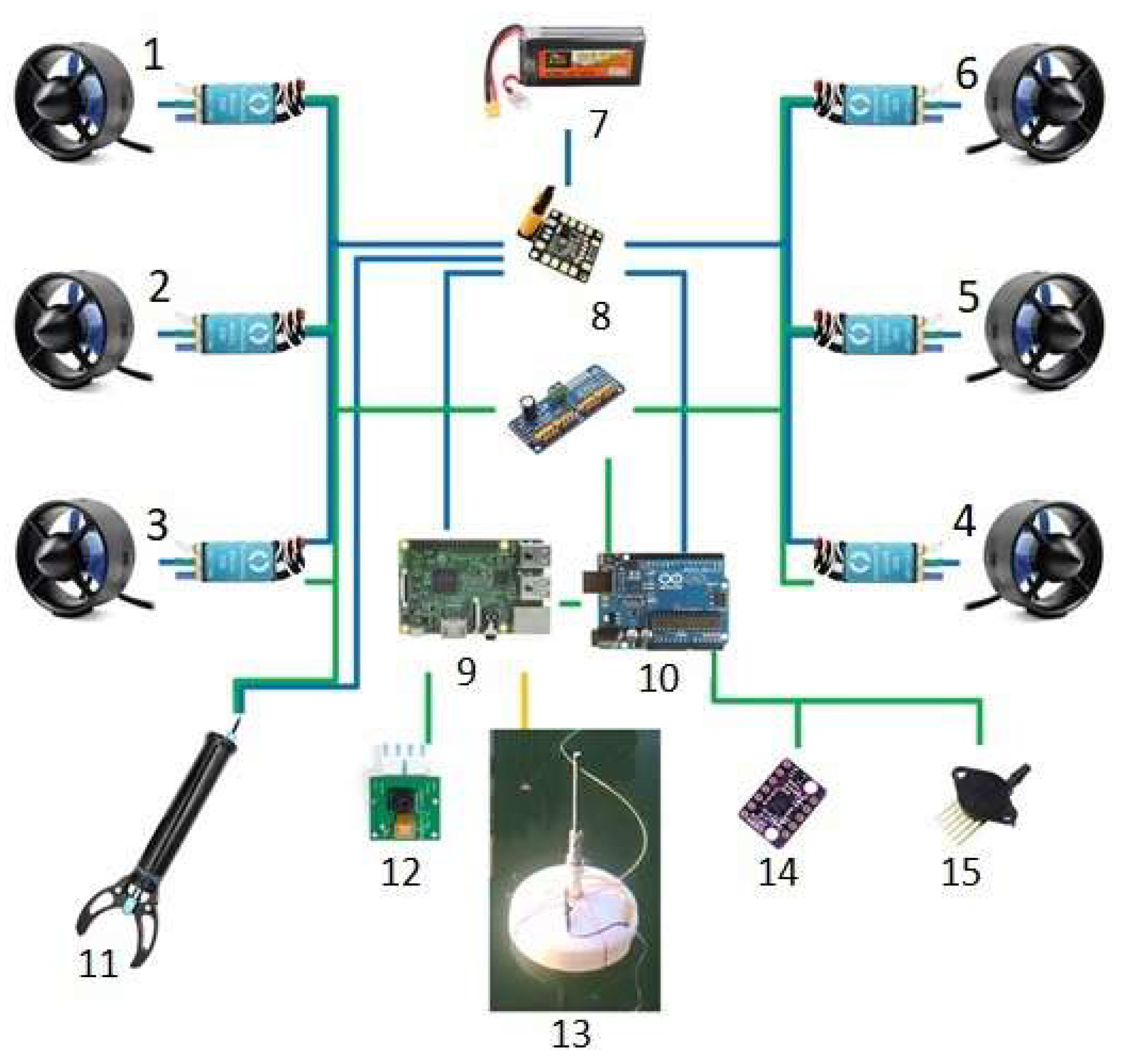
The purpose of the survey is to remotely conduct an automated set of measures to collect diagnostic data on the external state and the surroundings of an offshore gas pipeline. The monitoring systems can detect defects (such as damage) to the external coating, indentations and cracks on the pipe joints, erosion of the seabed, the presence of suspicious objects near the pipeline, and more. The functional diagram of the proposed automated remote survey system assumes there is an accompanying surface vessel (SV) [4], floating on the surface along the gas pipeline; the vessel also carries the UUV. The remotely controlled unmanned underwater vehicle “Vodyanoy-1” (our custom development) with the following functional modules (see Figure 2) is used as the UUV.

In Figure 2 the numbers indicate parts of the UUV as given below: 1–6 are the Motor drivers and T200 Thruster, 7 is the LiPo Battery, 8 is the Matek PDB-xt60, 9 is the Raspberry Pi, 10 is the Atmega328P, 11 is the Gripper, 12 is the Front NoIR Camera, for example, Basler camera acA1920-40gc (GigE interface, Sony IMX249 CMOS sensor, 42 fps @ 2.3 Mpix), 13 is the Wi-Fi Beacon, 14 is the IMU 9dof, 15 is the MPX5700. In addition, the UUV has the following attachable functional modules: overview sonar BlueView (to reconstruct 3D underwater scenes, avoid collisions, improve navigation accuracy), miniSVP sound velocity profile meter (to correct calculations). Various technical means and equipment for underwater robotic systems are given on site [5].

The paper [6] introduces a remotely operated underwater smart vehicle. The article demonstrates that smart features can be added to a dumb analogue remotely operated underwater drone by a small team of engineers on tight budget. This UUV maintains compass and depth headings, records video to an onshore terminal. In addition, vehicle has a remotely operated arm with 3 degrees of freedom. UUV “Malakhit” won the first prize on AquaRoboTech 2018 and remotely operated UUV “Vodyanoy-1” won the first AquaRoboTech 2020 competition and has a potential to be upgraded with advanced machine vision algorithms [7].

The article [8] examines the main stages of visual odometry in order to identify the factors that affect the quality of motion assessment, and establish the degree of their importance.

The main functionality of the software simulator developed of the visual odometry system are described. The paper presents the results of experiments conducted on the simulator, and infer certain conclusions out of them.

The functions between the SV (unmanned catamaran OceanAlpha M40 [7]) and the UUV are distributed as follows.

The SV provides:

• power supply for all equipment;
• scanning the bottom topography using the hydroecholocation system;
• global positioning receiver GNSS-H;
• local underwater positioning system (PS);
• wire communication via cable (CC) on an electric winch;
• wireless communication of the module via radio channel with the base station (BS) with Directional antenna, Network hardware;
• receiving and processing control commands.

The underwater vehicle can film underwater objects. Based on the data from the transponder (S), the positioning system calculates the vehicle’s coordinates and transmits them via a cable to the surface vehicle to provide autonomous underwater navigation. To improve the navigation accuracy of the underwater vehicle and to perform work on the 3D reconstruction of underwater scenes, in addition to a video camera, it is necessary to install an overview sonar.

The mobile operator station consists of a radio system, an operator’s workstation, and a server for recording and processing database data.

The inspection procedure is as follows.

The system receives control commands from the operator to launch certain scenarios. The scenarios are followed automatically, while the operator controls the process and only intervenes when anomalies are detected in the inspected object, or in the event of emergency situations in the system.

Let us highlight the following two basic scenarios to conduct surveys.

• Continuous. The underwater vehicle dives at the starting point. The SV begins to continuously move along the survey vector, scanning the bottom relief and the gas pipeline, while the UUV is simultaneously sailing behind it and filming the situation. Having reached the endpoint, the UUV ascends.
• Localized. The SV stops at a given fix. The UUV begins to sequentially dive, survey the surroundings, and ascend. Then the SV continues to move to the next checkpoint.

The operator’s mobile station can be additionally equipped with a software analytic system to automatically process the received data in real time to promptly adjust the survey control process.

The UUV carries out a set of measures to externally inspect the offshore section of the gas pipeline to determine its technical condition to detect defects and provide data to subsequently analyze the causes of defects and assess the technical condition of the gas pipeline and its surroundings. This procedure places high demands on the quality, reliability and uninterrupted operation of all components of the integrated automated system.

These requirements are especially stringent to one of the vulnerable components of the complex technology, namely for a remotely operated UUV. Therefore, an important and urgent problem is to assess the reliability characteristics of the underwater vehicle using advanced mathematical models.

The UUV can perform its functions as long as at least two engines located on opposite sides or any three engines are operational. Therefore, based on our agreement, the UUV can be considered as a k-out-of-$n:F$ system. The system consists of $n=6$ components, its failure depends on the position of its failed components, thus, it could be considered as a combination of $3+1$-out-of-$6:F$ and 5-out-of-$6:F$ systems. For such a system we will use special notation such as $(5,3+1)$-out-of-$6:F$ system.

1.3. Literature Review

Due to the wide practical application area, a lot of papers are devoted to the study of k-out-of-n– systems. The literature on such studies is vast and has been reviewed in [1] that is published in this issue. Thus, we will not repeat the review here, and because the paper is devoted to the problems of PM organization for the k-out-of-n models, we focus only on some works devoted to PM problems.

The idea to increase the system reliability by organizing the PM has a long story. A fairly detailed review of PM methods one can find in the monograph of Gertsbakh [9]. Some investigations of the k-out-of-n repairable systems with different strategies of repair and additional services have been considered in a series of work of Dudin, Krishnamurthy, and all [10,11,12,13,14,15]. Some recent developments on optimal maintenance policies can be found in [16,17,18,19,20].

Since detailed initial information about the reliability of system components is usually not available, it is fundamentally important to study the sensitivity of the system reliability indicators to the shape of system components lifetime distributions. Some research in this direction one can find in [21], in chapter 9 of [22], as well as in [23,24].

In this paper, we study and compare the effectiveness of different PM strategies for k-out-of-$n:F$ systems based on observation for their states. A feature of the model under consideration is the dependence of the system failure on the location of its failing components.

2. The Problem Set and Notations

2.1. The Notations and Assumptions

Consider a heterogeneous k-out-of-n:F system that is described in the Introduction. Denote by $A_i:i=1,2,\dots$ the sequence of the system components random lifetimes. Suppose that they are independent identically distribute (i.i.d.) random variables (r.v.’s) with the cumulative distribution function (c.d.f) $A\left(t\right)=\mathbf{P}\{A_i\le t\}$ the same for all of them. After any system failure it is repaired with a single facility and the repair times are i.i.d. r.v.’s $B_i^{\left(0\right)}:i=1,2,\dots$ with common c.d.f. $B_0\left(t\right)=\mathbf{P}\{B_i^{\left(0\right)}\le t\}$ and mean value

$$b_0=\mathbf{E}\left[B_0\right]={\int }_0^{\infty }(1-B_0\left(t\right))dt.$$

To increase the reliability of the system, the possibility of PM, based on the system states observation, is assumed. Let $\mathcal{L}=\{0,1,\dots ,L\}$ be a set of possible PM strategies including running to the system failure for $l=0$. For the l-th strategy denote by $E_l$ the system “pre-failure” subset of states, where l-th type of maintenance begins. The times of PM are i.i.d. r.v.’s $B_i^{\left(l\right)}$ with c.d.f. $B_l\left(t\right)=\mathbf{P}\{B_i^{\left(l\right)}\le t\}$ and mean value

$$b_l=\mathbf{E}\left[B_l\right]={\int }_0^{\infty }(1-B_l\left(t\right))dt.$$

The mean PM time $b_l$ is supposed to be less than the mean repair time $b_0, b_l\le b_0$, but may depend or not on the type of maintenance.

For investigation of reliability of the complex system, where failure depends not only on the number of its failed components but also on their position in the system, let us denote the system state by $\mathbf{j}=(j_1,j_2,\dots j_n)$, where $j_i=1$, if the i-th component is in “DOWN” state, and $j_i=0$, if the i-th component is in “UP” state. Thus, $j=j_1+\dots +j_n$ means number of failed components of the system. Let’s denote also

$$E=\{\mathbf{j}=(j_1,j_2,\dots j_n):(j_i\in (0,1))\}$$

to be the system set of states and by $E_0$ and ${\overline{E}}_0$ subsets of its “DOWN”‘and ‘UP” states accordingly. Note that the description of these sets is a special problem of concrete applications and should be considered for any special case.

It is supposed that

• in the very beginning the system is absolutely reliable, i.e. it is in zero state $\mathbf{j}=(0,\dots ,0)$;
• all sequences of r.v.’s (components lifetimes, repair, and PM times) are i.i.d. for each type of r.v.’s;
• after any repair and PM completion the system becomes “as a new one”, i.e., goes to the zero state1.

2.2. The Problem Set

The paper’s aim is to compare different PM strategies $l\in \mathcal{L}$ ( including running to the system failure for $l=0$) with respect to some criterion. As a criterion of the PM quality the system availability $K_{\mathrm{av}.,l}$ for different PM strategies $l\in \mathcal{L}$ is considered2,

$$K_{\mathrm{av}.,l}=\underset{t\to \infty }{lim}\frac{1}{t}\{\mathrm{the} \mathrm{system} \mathrm{working} \mathrm{time} \mathrm{during} \mathrm{time} t \mathrm{under} \mathrm{strategy} l\}.$$

For the stated problem solution, let us define a random process $J=\left\{\mathbf{J}\right(t):t\ge 0\}$ with the set of space E by the relation

$$\mathbf{J}\left(t\right)=\mathbf{j}, \mathrm{if} \mathrm{at} \mathrm{time} t \mathrm{system} \mathrm{is} \mathrm{in} \mathrm{the} \mathrm{state} \mathbf{j}\in E$$

and denote by $S_l (l\in \mathcal{L})$ time to the subset $E_l$ destination,

$$S_l=inf\{t:\mathbf{J}\left(t\right)\in E_l\}.$$

Thus, the value $S_0$ represents lifetime of the system and $S_l (l=\overline{1,L})$—the time till the l-th type maintenance beginning.

In the paper, we are interested to calculate different characteristics of the system, such as

• the system reliability function

  $$R\left(t\right)=\mathbf{P}\{S_0>t\} \mathrm{and} \mathrm{its} \mathrm{mean} \mathrm{value} M_0=\underset{0}{\overset{\infty }{\int }}R\left(t\right)dt.$$

  (1)
• distributions of time before starting different maintenance and their mean values

  $$F_l\left(t\right)=\mathbf{P}\{S_l\le t\},M_l=\underset{0}{\overset{\infty }{\int }}(1-F_l\left(t\right))dt.$$

  (2)
• the system availability $K_{\mathrm{av}.,l}$ for different PM strategies $l\in \mathcal{L}$.

Because the initial information about system components lifetime is usually very limited and available only up to one or two moments, we focus on the study of how sensitive is a decision on the PM quality to the shape of their distributions.

3. Process J and the General Procedure of the PM Quality Calculation

3.1. Process $\mathbf{J}$

Note first of all that due to our assumptions under any PM strategy, including running to the system failure, the process $\mathbf{J}$ is a regenerative one, where regenerative epochs are the times of maintenance or repair ends. Denote by ${\Pi }_0$ and ${\Pi }_l$ the process regeneration periods for the cases of the system working up to failure (for $l=0$) or under the l-th type $l=\overline{1,L}$ of maintenance. Thus, the system availability is

$$K_{\mathrm{av}.,0}=\frac{\mathbf{E}\left[S_0\right]}{\mathbf{E}\left[{\Pi }_0\right]},K_{\mathrm{av}.,l}=\frac{\mathbf{E}\left[S_l\right]}{\mathbf{E}\left[{\Pi }_l\right]}.$$

(3)

Therefore due to the properties of regenerative processes for availability $K_{\mathrm{av}.,l}$ calculation, we need only the mean value $\mathbf{E}\left[{\Pi }_l\right]$ of the regeneration period ${\Pi }_l$ and the mean value $M_l=\mathbf{E}\left[S_l\right]$ of the working time $S_l$ in it. Since for any PM strategy $l\in \mathcal{L}$, the regeneration period equals to

$${\Pi }_l=S_l+B_l,$$

and the mean repair and PM times $b_l=\mathbf{E}\left[B_l\right]$ are supposed to be known and measured in the same scale, for the problem solution we need only to calculate the distributions (or only the mean values) of the system working times $S_l$ for the case when it works to failure (for $l=0$) and for a system that operates under the l-th maintenance strategy.

3.2. The General Procedure of the PM Quality Calculation

For the solution of the declared problem, we need to calculate system availability $K_{\mathrm{av}.,l}$ for different preventive maintenance strategies $l\in \mathcal{L}$, including running to the system failure (for $l=0$). To do that we have to calculate c.d.f.’s (1, 2) of the subsets $E_l (l\in \mathcal{L})$ destination times. Note that the time $S_l (l\in \mathcal{L})$ of the subsets $E_l$ destinations coincides with the corresponding member of the variation series of the failure epochs of the system components. Therefore, for the solution of the stated problem, the following general algorithm should be used.

Remark 1.

The Algorithm 1 can also be used to solve other different problems, for example, to analyze if the preference of one strategy over another is sensitive to the shape of the system components lifetime distributions.

Further, the Algorithm 1 will be applied to several examples.

4. Homogeneous System Preventive Maintenance

4.1. Preliminary

Consider firstly a homogeneous k-out-of-n:F system, where failure does not depend on the configuration of its failed components. The subsets of UP and DOWN states of the system in this case are:

$${\overline{E}}_0=\{0,1,2,\dots ,k-1\}{E}_0=\{k,k+1,\dots ,n\}.$$

Let us define the subset $E_l$ for the PM $l\in \mathcal{L}$ beginning as a single state $E_l=\left\{l\right\}$ with $l\le k-1$. Thus, in this case we can investigate k strategies $l=\{0,1,\dots ,k-1\}$, where 0-strategy means allow the system to operate up to its failure.

In this case, the general Algorithm 1 gets essentially simpler because the time to the subset $E_l$ destination coincides with respective member $A_{\left(l\right)}$ of the variation series of the times to the system components failures $A_i:(i=\overline{1,n})$.

The analytical expressions for mean values $M_l$ are not always accessible. However, their numerical calculation in accordance with the Algorithm 1 is not too difficult and it will be proposed in the next subsection for the case of a k-out-of-$n:F$ system for $k=4, n=6$.

4.2. Numerical Results

To obtain the concrete results apply our Algorithm 1 to the 4-out-of-$6:F$-system that can be considered as a model for the example of the Section 1.2. In this case, only four strategies of system control are possible.

• Strategy 0 is that the system operates up to its failure.
• Strategy l ($l=$ 1, 2, 3) is to begin the PM when the system occurs in the state l.

In order to compare Strategy l with the Strategy 0 (to work without any PM up to the system failure), we need to know the ratio $\frac{b_l}{b_0}$. It is supposed that the values of mean repair and PM times $b_0, b_l$ as well as their ratios are known to a DM. Therefore, to make a decision about the preference of one strategy over the other, one only needs to know the ratios of the mean working time of the system $\frac{M_l}{M_0}$ for them. Let’s consider the respective ratios for an exponential distribution and compare different strategies of PM $l=\overline{1,L}$ with the strategy to work up to full system failure $l=0$ for different distributions and variations.

To conduct a numerical experiment, the program code on the MATLAB platform is generated. This computing environment is chosen due to a wide range of built-in functions, covering cdf functions and numerically evaluation of the integrals, including improper integrals. MATLAB additional advantage are simple plotting functions and friendly interface. The figures and the tables shown below in the article are the output of the developed program.

In order to investigate the sensitivity of the PM quality to the shape of the distribution of system components lifetime in numerical experiments, four types of distributions: exponential with parameter $\alpha$, $Exp(\alpha$), Gamma distribution, $\Gamma (\Theta ,k)$, Gnedenko-Weibull distribution, $GW(\lambda ,k)$ and log-normal distribution $LN(\mu ,{\sigma }^2)$ are considered.

The parameters of all distributions in experiments are chosen such that their expectations coincide for different distributions and equal to 1 (it means that we scaled it with respect to mean components lifetime), while the coefficient of variation $c=\frac{\sigma }{\mu }$ is varied in the interval $c\in [0.3,5.0]$.

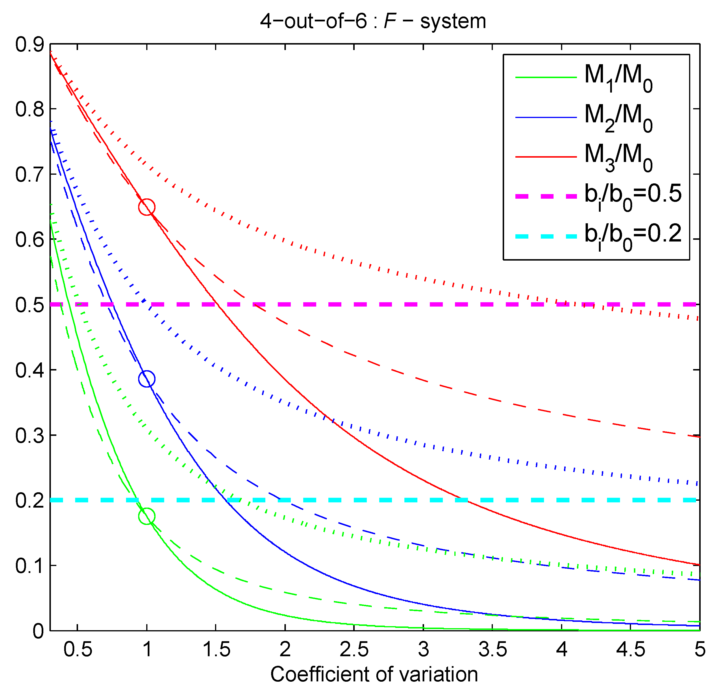
The results of the experiments are presented in Figure 3 and

Table 1. Boundary values for the coefficient of variation $c^{*}$ for 4-out-of-$6:F$ system.

Distribution	${\mathit{b}}_{\mathit{l}}/{\mathit{b}}_0=0.5$			${\mathit{b}}_{\mathit{l}}/{\mathit{b}}_0=0.2$
	$\mathbf{l}=\mathbf{1}$	$\mathbf{l}=\mathbf{2}$	$\mathbf{l}=\mathbf{3}$	$\mathbf{l}=\mathbf{1}$	$\mathbf{l}=\mathbf{2}$	$\mathbf{l}=\mathbf{3}$
$\Gamma$- distribution	0.44	0.76	1.51	0.93	1.57	3.30
$GW$-distribution	0.38	0.71	1.76	0.91	1.96	$>5$
Log-normal distribution	0.51	0.99	4.08	1.66	$>5$	$>5$

and

Table 2. Boundary values for the coefficient of variation $c^{**}$ to compare strategies $l=2$ and $l=3$ for 4-out-of-$6:F$ system.

Distribution	${\mathit{b}}_{\mathit{l}}/{\mathit{b}}_0=0.5$	${\mathit{b}}_{\mathit{l}}/{\mathit{b}}_0=0.2$
$\Gamma$-distribution	1.275	2.749
$GW$-distribution	1.427	>5
Log-normal distribution	3.771	>5

. In Figure 3 the ratios of mean working times $M_l$ under different PM strategies $l=1,2,3$ to mean working time $M_0$ for the system operating up to its failure ($l=0$) for different distributions of components lifetime versus the coefficient of variation are shown. Bold dashed horizontal lines correspond to the ratios of the mean PM time $b_l$ for any strategy l to mean repair time $b_0$. Intersections of these lines with the curves $M_l/M_0$ for different distributions determine the boundary values $c^{*}$ of the coefficient of variation, where the preference of appropriate strategy l is changed to the preference for “the system working up to the failure”. If the coefficient of variation exceeds the boundary value $c>c^{*}$ “the system working up to the failure” strategy ($l=0$) is preferable for given distribution, otherwise the appropriate PM strategy should be used.

Algorithm 1: General algorithm to choose a PM strategy

Start. Determine: Integers $n,k$, distribution $A\left(t\right)$ of components lifetime, subsets $E_l (l\in \mathcal{L})$ for the PM beginnings or of the system failure for $l=0$, mean PM and system repair times $b_l (l\in \mathcal{L})$. Step 1. Describe the duration of the subsets $E_l (l\in \mathcal{L})$ destinations in terms of members of the variation series, $$A_{\left(1\right)},\dots ,A_{\left(j\right)},\dots ,A_{\left(n\right)}$$ of the system components failure times (i.i.d r.v.) $A_1,\dots ,A_j,\dots ,A_n$ that bring the system to the subset $E_l$. Step 2. Calculate distributions of the respective members of the variation series $$A_{\left(j\right)}\left(t\right)=\mathbf{P}\{A_{\left(j\right)}\le t\}=\sum _{j\le i\le n}\left(\genfrac{}{}{0pt}{}{n}{i}\right)A^i\left(t\right){(1-A\left(t\right))}^{n-i}.$$ (4) Step 3. Calculate the distributions $F_l\left(t\right)$ of the subsets $E_l$ destination times in terms of distributions of respective series members and their expectations, $$M_l=\mathbf{E}\left[S_l\right]=\underset{0}{\overset{\infty }{\int }}(1-F_{\left(l\right)}\left(t\right))dt.$$ Step 4. Compare different PM strategies with respect to maximizing the system availability given by (3). We know that in terms of mean times to the destination of the respective subsets, the system availability can be represented as $$K_{\mathrm{av}.,l}=\frac{M_l}{M_l+b_l}$$ and because the l-th PM strategy is preferred over the j-th one if $K_{\mathrm{av}.,l}>K_{\mathrm{av}.,j}$ from the inequality $$\frac{M_l}{M_l+b_l}>\frac{M_j}{M_j+b_j}$$ it follows that the l-th strategy is preferred over the j-th one ($l\ge j$) if and only if $$M_l{b}_j>M_j{b}_l,\hspace{1em}\mathrm{or} \mathrm{in} \mathrm{terms} \mathrm{of} \mathrm{dimensionless} \mathrm{indexes}\frac{b_l}{b_j}<\frac{M_l}{M_j}.$$ (5) Step 5. Print results in terms of mean operational times $M_l(l\in \mathcal{L})$ and their ratio $\frac{M_j}{M_l}$ as advice to a Decision Maker (DM) in order to choose the best strategy accordingly to inequality (5). Stop.

The boundary values $c^{*}$ of the coefficient of variation when the PM strategy $l=1,2,3$ is preferable to strategy $l=0$ (running to the system failure) for two values of the ratios mean PM duration $b_l$ to mean repair time $b_l/b_0=0.5$ (upper horizontal line in Figure 3) and $b_l/b_0=0.2$ (lower horizontal line in Figure 3) for different distributions of system components lifetime are represented in the Table 1.

The Figure 3 demonstrates an almost evident fact that the highest value of the ratios $\frac{M_l}{M_0}$ is achieved for $l=3$, which means that the strategy $l=3$ is preferable over other strategies in the case when all mean PM times are equal, $b_l=b$ for $l=1,2,3$. Moreover this strategy will be better than the strategy $l=0$ “the system runs to failure” until the coefficient of variation is less than the boundary value $c^{*}$ for any specified ratio $\frac{b}{b_0}$. If the coefficient of variation $c>c^{*}$ strategy $l=0$ will be preferable to all others.

However, depending on the coefficient of variation, the decision about the choice of the PM is sensitive to the distribution of system components lifetime. With an increase in the coefficient of variation, the ratio $M_l/M_0$ decreases, but the difference between distributions grows.

Suppose the repair time is twice longer than PM time (the violet line in Figure 3). Assuming an exponential distribution of components lifetime, $l=3$ is preferable for 4-out-of-$6:F$ system. The decision for other distributions of components lifetime depends on the coefficient of variation. If $c>1.51$ for $\Gamma$-distribution or $c>1.76$ for $GW$-distribution, the strategy $l=0$ should be chosen. In case components lifetime follows a log-normal distribution, the strategy $l=0$ should be chosen if $c>4.08$.

If the repair time is five times longer than PM time (the cyan line in Figure 3) and the coefficient of variation is no greater than 3.3, the strategy $l=3$ will be the best regardless of the type of components lifetime distribution. However, as it is possible to see from Figure 3, for $c>3.3$ the choice of the strategy significantly depends on the components lifetime distribution.

In case of different mean PM times $b_l$, strategies $l=1,2,3$ can be compared one with another. We compare the strategies $l=2$ and $l=3$ for the studied distributions, and present the results in Table 2. The table provides the boundary values for the coefficient of variation $c^{**}$, where the preference for the strategy $l=2$ is changed to the preference for the strategy $l=3$ for $b_2/b_3=0.5$ or $b_2/b_3=0.2$. If the coefficient of variation exceeds the boundary value $c>c^{**}$ the strategy $l=3$ “to start PM after 3 components failure” for given distribution is preferable. Otherwise the strategy $l=2$ “to start PM after 2 components failure” should be used. So according to the Table 2 if the PM time for $l=3$ is twice as much as the PM time for $l=2$ and $\Gamma$-distribution with the coefficient of variation $c>1.275$ is taken, the strategy $l=3$ is better than the strategy $l=2$. The same conclusion can be made if components lifetime follows $GW$-distribution and $c>1.427$, and for log-normal distribution if $c>3.771$. If the PM time for $l=3$ is five times longer than the PM time for $l=2$ assuming $GW$- or log-normal distribution, the strategy $l=2$ is preferable for the whole interval $c\in [0.3,5.0]$, and for a $\Gamma$- distribution it will be the best choice if $c<2.749$.

Thus, the conducted study allows us to draw the following conclusions regarding the sensitivity of the decision on the choice of a PM strategy to the type of distributions of the system components lifetime and the coefficient of variation.

At low values of the coefficient of variation, strategies with PM gain an advantage over the strategy of working until complete system failure and repair (in terms of a higher value of the availability factor). It is possible to distinguish intervals of values of the coefficient of variation where the conclusion about the use of the certain strategy will be the same for any of the considered distributions.

$\Gamma$-distribution and $GW$-distribution have insignificant differences in $M_l/M_0$ when the coefficient of variation is in the interval $c\in [0.3,1.1]$, the log-normal distribution tends to widen the range of the coefficient of variation values when the strategy $l=3$ can be adopted as the preferred strategy in comparison to $l=0$.

Calculated with Matlab, the system mean working times under different PM strategies and the mean system operational time until its failure (for $l=0$) for the special case of the exponential distribution of components lifetime with parameter $\alpha =1$ are: $M_1=0.1667, M_2=0.3667, M_3=0.6167, M_0=M_4=0.95.$ Corresponding ratios are

$$\frac{M_1}{M_0}=0.1754,\frac{M_2}{M_0}=0.386,\frac{M_3}{M_0}=0.649.$$

These values, calculated for the exponential distribution, are marked with circles in Figure 3. Consequently, the strategy $l=2$ is better than $l=0$ if the system repair time $b_0$ is $\frac{1}{0.386}\approx 2.6$ or more times longer than the mean PM time $b_2$. The ratios to compare strategies $l=1$ and $l=2$ or $l=2$ and $l=3$ are also shown below

$$\frac{M_1}{M_2}=0.454,\frac{M_2}{M_3}=0.595.$$

The strategy $l=2$ is better than $l=1$ if the mean PM time $b_1$ is not less than $45.4\%$ of the mean PM time $b_2$.

However, due to the properties of an exponential distribution, this case can be studied analytically, as it is shown in the next subsection.

4.3. Special Case: Exponential Distribution of Components Lifetime

Under the assumption about an exponential distribution of the lifetimes of the system components $A_i$,

$$A\left(t\right)=\mathbf{P}\{A_i\le x\}=1-e^{-\alpha t},$$

due to the independence of the residual lifetimes of all other components on the failure time of any one of them, another approach is possible. In this case, the intervals $T_i$ between the $i-1$-th and the i-th failures are

$$T_i=min\{A_1,A_2,\dots A_{6-(i-1)}\},$$

and therefore

$$F_i\left(t\right)=\mathbf{P}\{T_i\le t\}=1-\mathbf{P}\{T_i>t\}=1-{(1-A\left(x\right))}^{6-i}=1-e^{(6-(i-1\left)\right)\alpha t}.$$

Thus, it holds $m_i=\mathbf{E}\left[T_i\right]={\left[(6-(i-1))\alpha \right]}^{-1}$ and therefore

$$\frac{M_1}{M_2}=\frac{m_1}{m_1+m_2}=\frac{\frac{1}{6\alpha }}{\frac{1}{6\alpha }+\frac{1}{5\alpha }}=\frac{5}{11}\approx 0.4545.$$

From here it follows that the necessary and sufficient condition (5) for the first PM to be preferable over the second one is

$$\frac{b_1}{b_2}>\frac{M_1}{M_2}\approx 0.4545,$$

or the mean time of the second strategy PM should be more than twice longer than the relevant value for the first one. Analogously the inequality

$$\frac{b_2}{b_0}>\frac{M_2}{M_4}=\frac{m_1+m_2}{m_1+m_2+m_3+m_4}=\frac{\frac{1}{6\alpha }+\frac{1}{5\alpha }}{\frac{1}{6\alpha }+\frac{1}{5\alpha }+\frac{1}{4\alpha }+\frac{1}{3\alpha }}=\frac{22}{57}\approx 0.386$$

shows that the second PM strategy is preferable to the system running to its failure with the following repair only if its mean PM time is less than 38% of the mean repair time. The results of this section are in complete agreement with the numerical calculations given for exponential distribution in Section 4.2.

5. Preventive Maintenance of a System, Where Failures Depend on the Location of the Failed Components

5.1. Preliminary

If the system failure depends on the location of the failed components, the comparison of strategies, including “running to the system failure”, and the decision about the choice of PM are system-specific and depend on the exploitation conditions. Thus, it is impossible to solve these problems in general settings. Therefore, in this section we consider this problem for the concrete $(3+1,5)$-out-of-$6:F$ system with specific conditions of its exploitation.

5.2. Example: Model $(3+1,5)$-out-of-$6$

Turn back to the investigation of the model that has been proposed in Section 1.2 under the condition that the system fails, when four (moreover three from one side and one from the other side) or five motors fail. In other words, it means that the system operates if any three or at least one from one side and one from the other side of its motors operate. Thus, this system could be considered as a combination of $3+1$-out-of-$6:F$ and 5-out-of-$6:F$ systems. For simplicity in Section 1.2 for such kind of systems a special notation $(3+1,5)$-out-of-$6:F$ system is proposed.

For the convenience, a binary code is used to indicate system states, namely the number of the state $\mathbf{j}=(j_1,j_2,\dots j_6)$ is given in accordance with the formula

$$j=\left|\mathbf{j}\right|=\sum _{0\le i\le 6}{j}_i{2}^{6-i}.$$

Then the subset of failure states $E_0$ includes the states with the numbers

$$E_0=\{\mathbf{15},\mathbf{23},31,\mathbf{39},47,55,\mathbf{57},\mathbf{58},59,\mathbf{60},61,62,63\},$$

where the states with 3 failures on the same side and 1 on the other are highlighted in bold. By analogy with how it is defined in Section 4.2 consider four strategies:

• Strategy 0 is to run to the system failure (do not use any PM). It means that the repair begins when 4 failures occur at that 3 of them on one side and one on the other or 5 failures occur. The subset of the states for the repair beginning is $E_0$.
• Strategy $l (l=1,2,3)$ is to begin the PM after the failure of any l components.

In this case the ordinal statistics do not determine uniquely the distribution time to the corresponding subset of states destination. Thus, the Algorithm 1 takes the following form.

5.3. Numerical Analysis

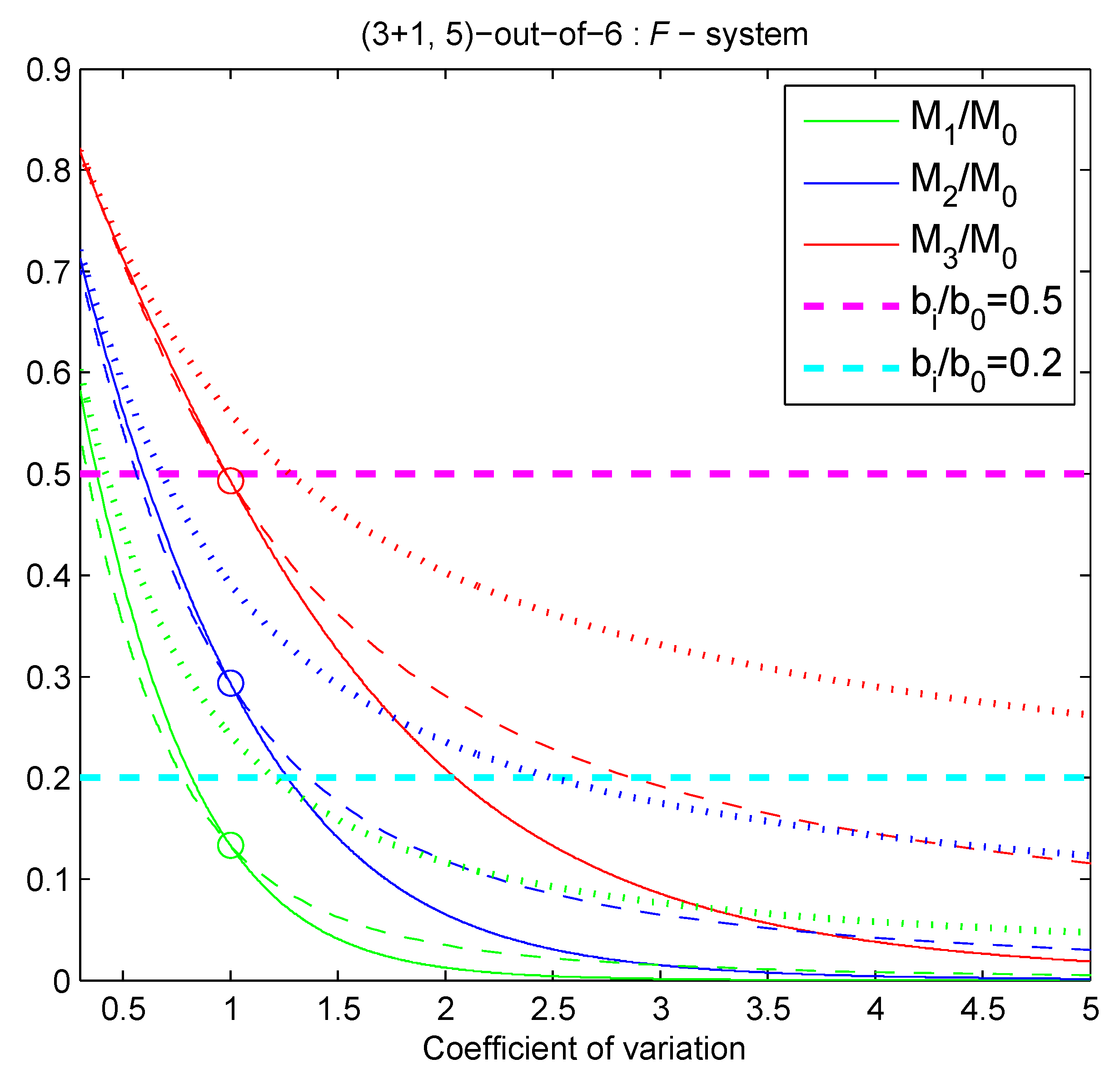
The results of the numerical experiments performed in accordance with Algorithm 2 are presented in Figure 4 and

Table 3. Boundary values for the coefficient of variation $c^{*}$ for $(3+1,5)$-out-of-$6:F$ system.

Distribution	${\mathit{b}}_{\mathit{l}}/{\mathit{b}}_0=0.5$			${\mathit{b}}_{\mathit{l}}/{\mathit{b}}_0=0.2$
	$\mathbf{l}=\mathbf{1}$	$\mathbf{l}=\mathbf{2}$	$\mathbf{l}=\mathbf{3}$	$\mathbf{l}=\mathbf{1}$	$\mathbf{l}=\mathbf{2}$	$\mathbf{l}=\mathbf{3}$
$\Gamma$-distribution	0.37	0.6	0.98	0.82	1.26	2.05
$GW$-distribution	0.34	0.56	0.98	0.78	1.36	2.85
Log-normal distribution	0.42	0.68	1.27	1.2	2.49	$>5$

. As in the previous case (Section 4.2) in Figure 4 the ratios $\frac{M_l}{M_0}$ of mean system working times $M_l$ under different strategies $l=1,2,3$ to mean system working time $M_0$ up to its failure ($l=0$) for different distributions of system components lifetime versus the coefficient of variation for $(3+1,5)$-out-of-$6:F$ system are given. Four failure distributions: $\Gamma$-distribution, $GW$-distribution, log-normal distribution, and exponential distribution are examined. Bold dashed horizontal lines correspond to the ratios of the mean PM time $b_l$ for any PM strategy l to the mean repair time $b_0$. The intersections of these lines with curves $M_l/M_0$ for different distributions determine the boundary values $c^{*}$ of the coefficient of variation, where the preference of appropriate strategy l is changed to the preference for the strategy “the system running to the failure” ($l=0$). If the coefficient of variation exceeds the boundary value $c>c^{*}$, the strategy $l=0$ for given distribution is the preferable one. Otherwise appropriate PM strategy l should be chosen. The boundary values $c^{*}$ of the coefficient of variation when PM strategy $l=1,2,3$ is preferable to strategy $l=0$ for $b_l/b_0=0.5$ (upper horizontal line in Figure 4) and $b_l/b_0=0.2$ (lower horizontal line in Figure 4) for the two values $b_l/b_0=0.5$ and $b_l/b_0=0.2$ numerically calculated for different distributions of system components lifetime are represented in Table 3.

Figure 4 shows that the difference between distributions grows as the coefficient of variation increases. So, depending on the coefficient of variation, the decision about the choice of the PM is sensitive to the distribution of system components lifetime.

Since collection of data on real equipment failures takes considerable time and the confidence intervals for the mathematical expectation and standard deviation of the investigated random variables can be wide enough, it makes sense when choosing the best strategy to focus not on a specific value of the coefficient of variation, but on the range $c\in [c_{min},c_{max}]$, and make a decision on the choice of a strategy on the assumption that the coefficient of variation can be in the specified range. For example, with the ratio of PM time to repair time $b_l/b_0=0.2$ if the variation coefficient is supposed to be in the interval $c\in [0.3,2.05]$, the strategy $l=3$ will be the best for any of the considered distributions. For $c\in [2.05,2.85]$ for a $\Gamma$-distribution of the system components lifetime, one should prefer the strategy of operation until complete failure $l=0$, for a $GW$- and a log-normal distributions strategy $l=3$ will remain the best. For $c\in [2.85,5]$ the strategy $l=0$ should be chosen for a $\Gamma$- and a $GW$- distributions. For a log-normal distribution the choice is the strategy $l=3$ regardless the coefficient of variation. So the choice of the strategy significantly depends on the distribution of components lifetime.

Algorithm 2:The choice of a PM strategy for a heterogeneous system

Start is repeated from the Algorithm 1. Step 1. Determine the times to set of states $E_l$ destination in terms of ordinal statistics $A_{\left(j\right)}$. Because the system failure occurs when 4 (3+1) or 5 motors fail, so the time $S_0$ to the subset $E_0$ destination has the following form $$S_0=\left\{\begin{array}{c}{A}_{\left(4\right)}, \mathrm{if} \mathrm{four} \mathrm{motors} \mathrm{fail}, \mathrm{at} \mathrm{that} \mathrm{three} \mathrm{from} \mathrm{one} \mathrm{side} \mathrm{and} \mathrm{one} \mathrm{from}\hfill \\ \mathrm{the} \mathrm{other} \mathrm{side} (3+1),\hfill \\ A_{\left(5\right)}, \mathrm{if} \mathrm{four} \mathrm{motors} \mathrm{fail}, \mathrm{at} \mathrm{that} \mathrm{two} \mathrm{from} \mathrm{one} \mathrm{side} \mathrm{and} \mathrm{two} \mathrm{from} \mathrm{the}\hfill \\ \mathrm{other} \mathrm{side} (2+2), \mathrm{and} \mathrm{the} \mathrm{system} \mathrm{failure} \mathrm{occurs} \mathrm{after} \mathrm{the} \mathrm{fifth} \mathrm{failure}.\hfill \end{array}\right.$$ The times $S_l$ to the subsets $E_l(l=1,2,3)$ destination coincide with the relevant variation series members, namely: $$S_l=A_{\left(l\right)},\mathrm{the}\mathrm{PM}\mathrm{under}\mathrm{strategy}l\mathrm{begins}\mathrm{after}\mathrm{the}\mathrm{failure}\mathrm{of}l\mathrm{motors}.$$ Step 2. Calculate the distributions of times to the corresponding subsets destination in terms of the ordinal statistics distributions. Since the system failure occurs when (3+1) or 5 motors fail, and (3+1) failures state contains 6 of the 15 states from the complete subset $E_4$ of states with 4 failures, taking into account that the probabilities of any component failures are equal, so the probability of time to the destination of subset $E_0$ has a form $$F_0\left(t\right)=\frac{2}{5}{A}_{\left(4\right)}\left(t\right)+\frac{3}{5}{A}_{\left(5\right)}\left(t\right).$$ The distributions of the subset of states $E_l (l=1,2,3)$ destination are $$F_1\left(t\right)=A_{\left(1\right)}\left(t\right),F_2\left(t\right)=A_{\left(2\right)}\left(t\right),F_3\left(t\right)=A_{\left(3\right)}\left(t\right),$$ where accordingly to (4) distributions $A_{\left(j\right)}\left(t\right)$ are $$A_{\left(j\right)}\left(x\right)=\mathbf{P}\{X_{\left(j\right)}\le x\}=\sum _{j\le i\le n}\left(\genfrac{}{}{0pt}{}{n}{i}\right)A^i\left(x\right){(1-A\left(x\right))}^{n-i}.$$ Step 3. Calculate the expectations times to destinations of the subsets $E_l$. $$M_0=\frac{2}{5}\mathbf{E}\left[A_{\left(4\right)}\right]+\frac{3}{5}\mathbf{E}\left[A_{5)}\right],M_1=\mathbf{E}\left[A_{\left(1\right)}\right],M_2=\mathbf{E}\left[A_{\left(2\right)}\right],M_3=\mathbf{E}\left[A_{\left(3\right)}\right].$$ Step 4. With the help of obtained values compare different PM strategies using the necessary and sufficient condition to prefer the j-th strategy over the l-th one in the form of inequality (5). Step 5. Print results in terms of mean operational times $M_l (l\in \mathcal{L})$ and their ratio $\frac{M_j}{M_l}$ as advice to a DM in order to choose the best strategy. Stop.

5.4. Special Case

In the special case of exponential system components lifetime distribution, it is possible to use the same approach as before and the problem can be solved analytically.

In this case the time $S_2$ of the subset $E_2$ destination coincides with the distribution of the second ordinal statistics $A_{\left(2\right)}$, but it also equals the sum $S_2=T_1+T_2$ of the time to the first component failure $T_1$ and the time interval between the first and the second component failure $T_2$, where the distributions are exponential with parameters $6\alpha$ and $5\alpha$. Thus, the mean time to the second component failure is

$$M_2=m_1+m_2=\frac{1}{6\alpha }+\frac{1}{5\alpha }=\frac{11}{30\alpha }$$

Analogously the mean time to the subset $E_3$ destination is

$$M_3=m_1+m_2+m_3=\frac{1}{6\alpha }+\frac{1}{5\alpha }+\frac{1}{4\alpha }=\frac{37}{60\alpha }$$

Thus, the condition (5) of preference of the strategy $l=2$ to the strategy $l=3$$K_{\mathrm{av}.,2}>K_{\mathrm{av}.,3}$ takes the form

$$\frac{b_2}{b_3}>\frac{m_1+m_2}{m_1+m_2+m_3}=\frac{22}{37}\approx 0.59.$$

This means that the strategy $l=2$ will be preferable to the strategy $l=3$ if the mean PM time $b_2$ is less than 59% of $b_3$. This result coincides with the one we obtained for the corresponding strategies for the 4-out-of-$6:F$ system examined in Section 4.3 as the states with 2 or 3 failures are the same for both systems, the difference will be only in calculating the mean time before system failure with the following repair.

Compare now each of PM strategy with the regime of the system operating up to its failure with the following repair. To do that we should compare the mean times $M_l(l=2,3)$ of the subsets $E_l(l=2,3)$ destination with the mean time $M_0$ of the system operation up to its failure without any PM.

$$M_0=\frac{2}{5}\mathbf{E}\left[A_{\left(4\right)}\right]+\frac{3}{5}\mathbf{E}\left[A_{5)}\right]=\frac{2}{5}{M}_4+\frac{3}{5}{M}_5=\frac{2}{5}\frac{57}{60\alpha }+\frac{3}{5}\frac{87}{60\alpha }=\frac{5}{4\alpha }$$

The comparison shows that the strategy $l=2$ is preferable over working without PM $2\ge 0$ iff

$$\frac{b_2}{b_0}\ge \frac{M_2}{M_0}=\frac{22}{75}\approx 0.29$$

and the strategy $l=3$ is preferable over the working without PM iff

$$\frac{b_3}{b_0}\ge \frac{M_3}{M_0}=\frac{37}{75}\approx 0.49.$$

In Figure 4 the blue circle corresponds to the ratio $\frac{b_2}{b_0}=0.29$ and the red circle corresponds to the ratio $\frac{b_3}{b_0}=0.49$ which demonstrates the coincidence of analytical and numerical calculations for exponential distribution.

6. Conclusions

In this paper we investigate different PM strategies for a k-out-of-n system based on its states. The novelty and the feature of the paper are that the system failure depends on the position of its failed components. We propose a new method to solve this problem, based on the distribution of the members of the variational series of the failing components. Also, we investigated how sensitive the decision about PM beginning is to the shape of the system components’ lifetime distributions. This investigation is very actual because the initial information about system components lifetime is usually very limited and available only up to one or two moments.

We propose an algorithm to compare different PM strategies and to choose the best among them with respect to the system availability maximization. The algorithm can be used for any k-out-of-$n:F$ system with any system failure set. The algorithm is applied to analyze PM strategies of the UUV to monitor the condition of a subsea pipeline. A series of numerical experiments made it possible to draw conclusions about how sensitive the choice of PM strategy to the shape of system components lifetime distribution. It is also possible to determine the intervals for the coefficient of variation, where the decision to choose a preferable strategy does not depend on the type of distribution.

The proposed approach can be expanded with other quality criteria, such as productivity of the system or system service cost under different PM strategies. Multi-criteria assessment of the PM effectiveness is also possible.

References

- Rykov, V.V.; Sukharev, M.G.; Itkin, V.Y. Investigations of k-out-of-n systems application possibilities to objects of oil and gas industry. Mar. Sci. Eng. 2020, 8, 928. [Google Scholar] [CrossRef]
- Shepherd, D.K. k-out-of-n Systems. In Encyclopedia of Statistics in Quality and Reliability; American Cancer Society: Atlanta, GA, USA, 2008; Available online: https://0-onlinelibrary-wiley-com.brum.beds.ac.uk/doi/pdf/10.1002/9780470061572.eqr342 (accessed on 26 February 2019).
- Gazprom. Dzhubga—Lazarevskoye—Sochi. The First Russia-Based Offshore Gas Pipeline. Available online: https://www.gazprom.com/projects/dls/ (accessed on 19 November 2020).
- OceanAlpha Group Ltd. Autonomous Hydrographic Survey Boat. Available online: https://www.oceanalpha.com/product-item/m40/ (accessed on 19 November 2020).
- Blue Robotics. BlueROV2. Available online: https://bluerobotics.com/product-category/rov/bluerov2/ (accessed on 19 November 2020).
- Farkhadov, M.; Abramenkov, A.; Abdulov, A.; Eliseev, A. Portable Remotely Operated Underwater Smart Vehicle with a Camera and an Arm. In Proceedings of the 2019 10th International Power Electronics Drive Systems and Technologies Conference (PEDSTC), Shiraz, Iran, 12–14 February 2019; pp. 178–183. [Google Scholar] [CrossRef]
- Advanced Research Foundation. AquaRoboTech 2020 Competition. Available online: http://aquarobotech.ru/about (accessed on 19 November 2020).
- Abdulov, A.; Abramenkov, A. Visual odometry system simulator. In Proceedings of the 2017 International Siberian Conference on Control and Communications (SIBCON), Astana, Kazakhstan, 29–30 June 2017; pp. 1–5. [Google Scholar]
- Gertsbakh, I. Preventive Maintenance Models Based on the Lifetime Distribution. In Reliability Theory with Applications to Preventive Maintenance; Springer: Berlin/Heidelberg, Germany, 2000; pp. 67–106. [Google Scholar]
- Dudin, A.N.; Krishnamoorthy, A.; Narayanan, V.C. Idle time utilization through service to customers in a retrial queue maintaining high system reliability. J. Math. Sci. 2013, 191, 506–517. [Google Scholar] [CrossRef]
- Krishnamoorthy, A.; Viswanath, C.N.; Deepak, T.G. Reliability of a k-out-of-n-system with Repair by a Service Station Attending a Queue with Postponed Work. Int. J. Reliab. Qual. Saf. Eng. 2007, 14, 379–398. [Google Scholar] [CrossRef]
- Krishnamoorthy, A.; Viswanath, C.N.; Deepak, T.G. Maximizing of Reliability of a k-out-of-n-system with Repair by a facility attending external customers in a Retrial Queue. Reliab. Theory Appl. 2007, 2, 21–33. [Google Scholar]
- Krishnamoorthy, A.; Sathian, M.K.; Viswanath, C.N. Reliability of a k-out-of-n system with repair by a single server extending service external customers with pre-emption. Reliab. Theory Appl. 2016, 11, 61–93. [Google Scholar]
- Krishnamoorthy, A.; Sathian, M.K.; Viswanath, C.N. Reliability of a k-out-of-n system with a single server extending non-preemptive service to external customers- Part I. Reliab. Theory Appl. 2016, 11, 62–75. [Google Scholar]
- Krishnamoorthy, A.; Sathian, M.K.; Viswanath, C.N. Reliability of a k-out-of-n system with a single server extending non-preemptive service to external customers-Part II. Reliab. Theory Appl. 2016, 11, 76–88. [Google Scholar]
- Finkelstein, M.; Levitin, G. Preventive maintenance for homogeneous and heterogeneous systems. Appl. Stoch. Model. Bus. Ind. 2019, 35, 908–920. [Google Scholar] [CrossRef]
- Finkelstein, M.; Cha, J.H.; Levitin, G. On a new age-replacement policy for items with observed stochastic degradation. Qual. Reliab. Eng. Int. 2020, 36, 1132–1146. [Google Scholar] [CrossRef]
- Park, M.; Lee, J.; Kim, S. An optimal maintenance policy for k-out-of-n system without monitoring component. Qual. Technol. Qual. Manag. 2019, 16, 140–153. [Google Scholar] [CrossRef]
- Endharth, A.J.; Yun, W.Y.; Yamomoto, H. Preventive maintenance policy for linear-consequtive -k-out-of-n:F system. J. Oper. Res. Soc. Jpn. 2016, 59, 334–346. [Google Scholar]
- Hamdan, K.; Tavangar, M.; Asadi, M. Optimal preventive maintenance for repairable weighted k-out-of-n systems. Reliab. Eng. Syst. Safe 2021, 205, 107267. [Google Scholar] [CrossRef]
- Kozyrev, D.; Kolev, N.; Rykov, V. Reliability function of renewable system under marshall-lkin Failure Model. Reliab. Theory Appl. 2018, 13, 39–46. [Google Scholar]
- Rykov, V. On Reliability of Renewable Systems. In Reliability Engineering. Theory and Applications; Vonta, I., Ram, M., Eds.; CRC Press: Boca Raton, FL, USA, 2018; pp. 173–196. [Google Scholar]
- Rykov, V.; Kozyrev, D. On the reliability function of a double redundant system with general repair time distribution. Appl. Stoch. Model. Bus. Ind. 2019, 35, 191–197. [Google Scholar] [CrossRef]
- Rykov, V.; Kozyrev, D.; Filimonov, A.; Ivanova, N. On reliability function of a k-out-of-n system with general repair time distribution. Probab. Eng. Inf. Sci. 2020, 5, 1–18. [Google Scholar] [CrossRef]