Comparative Analysis of Environmental Contour Approaches to Estimating Extreme Waves for Offshore Installations for the Baltic Sea and the North Sea

 ,
,  , , , and
Abstract
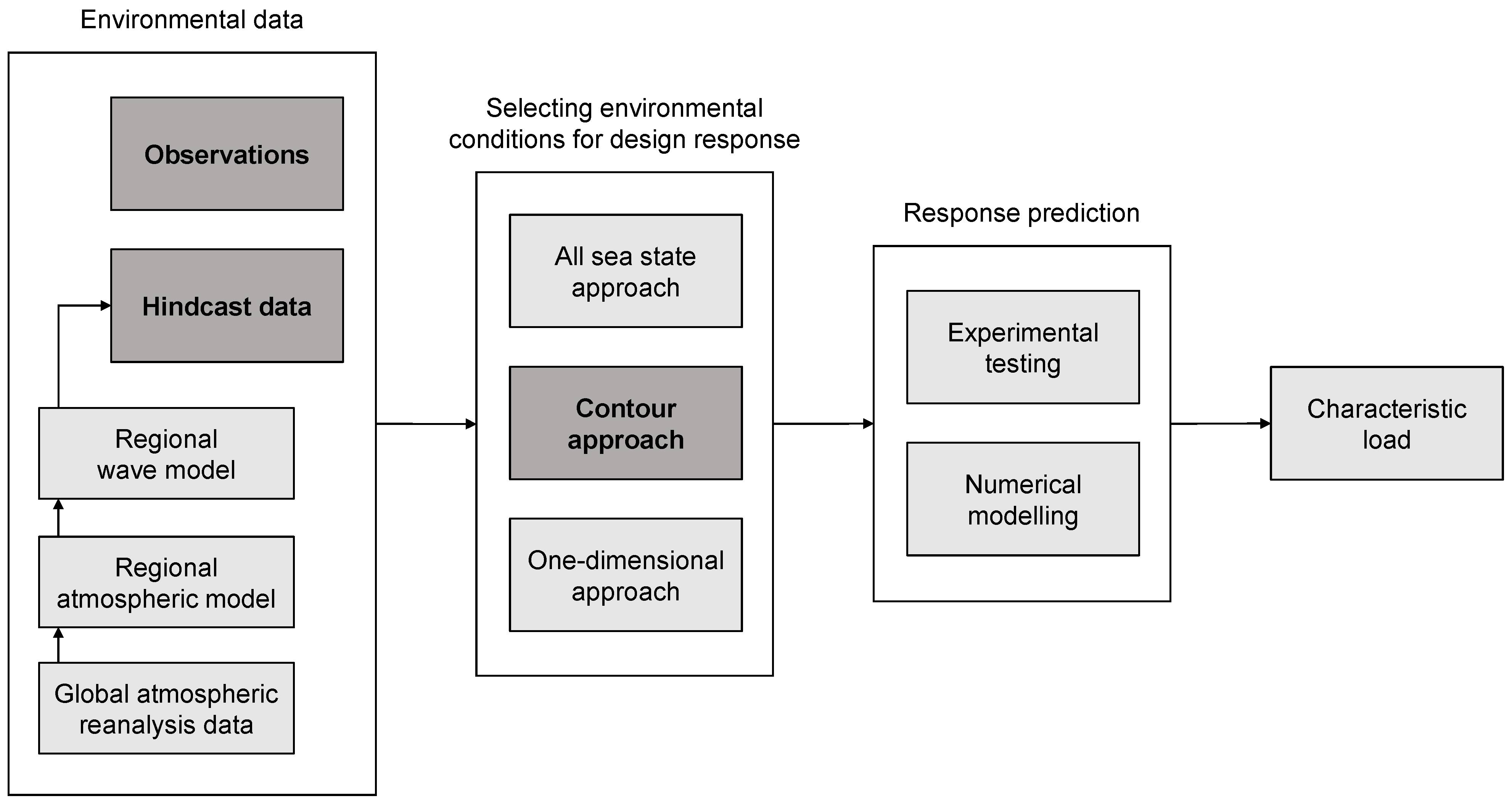
:1. Introduction
2. Data
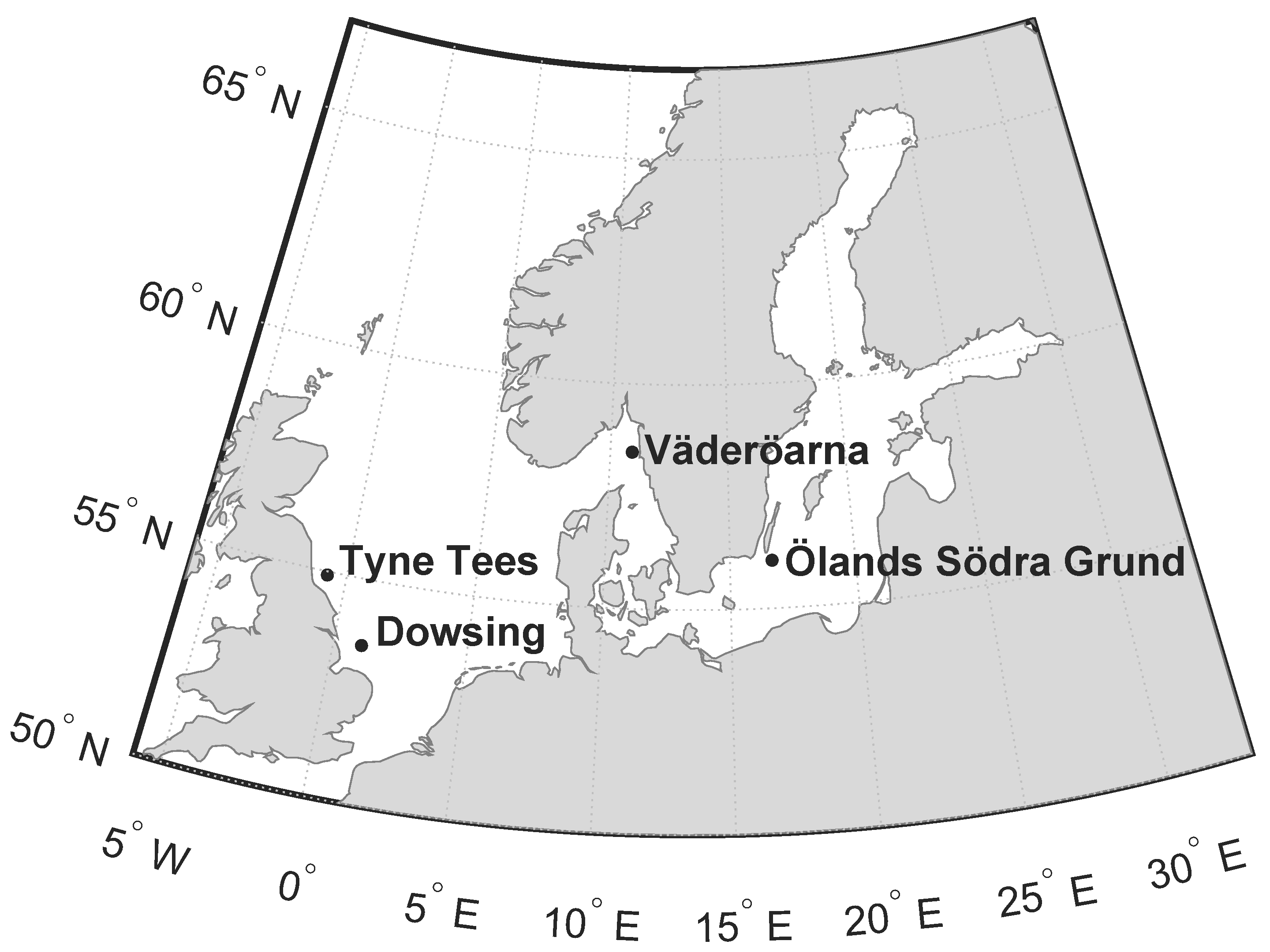
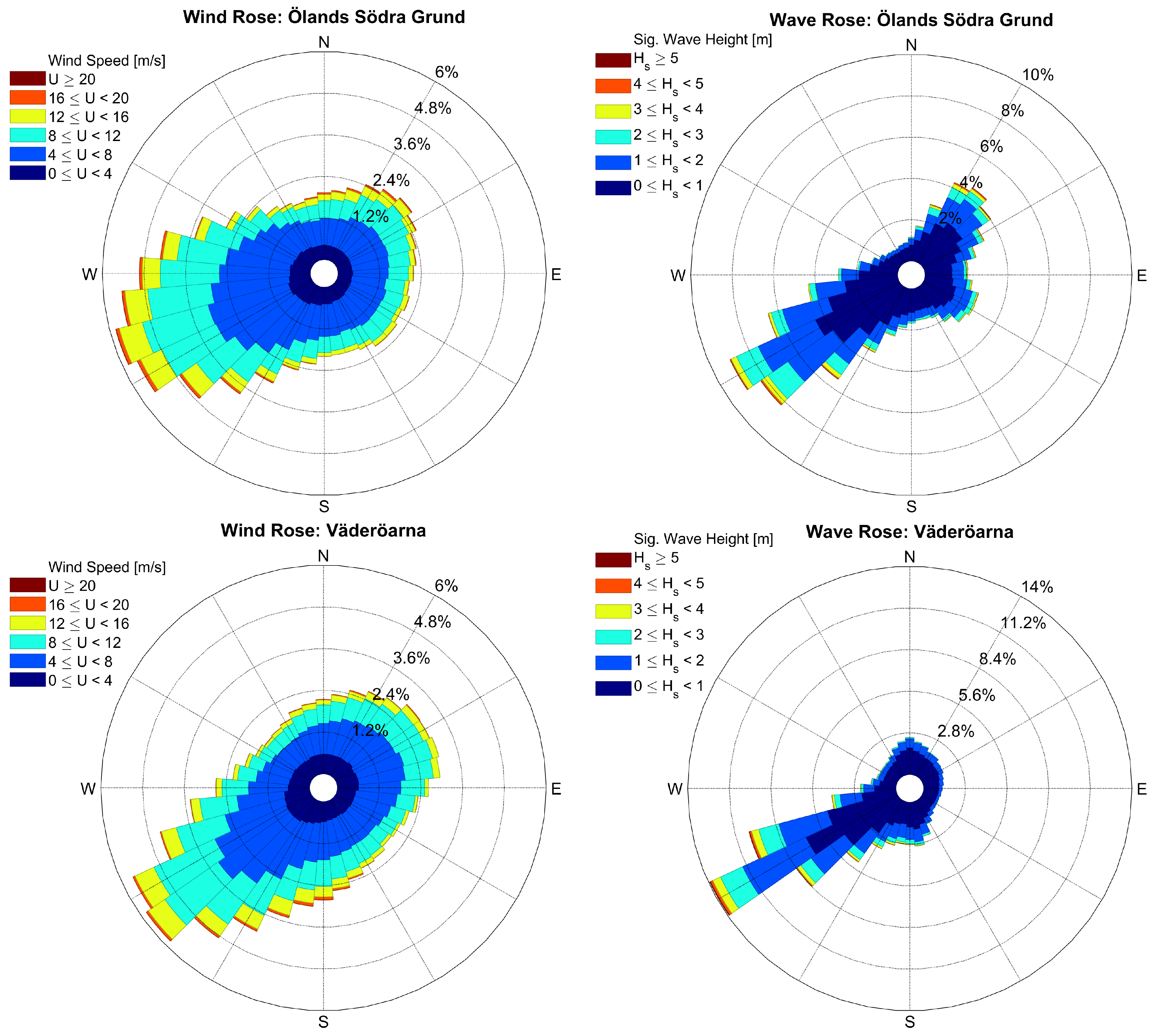
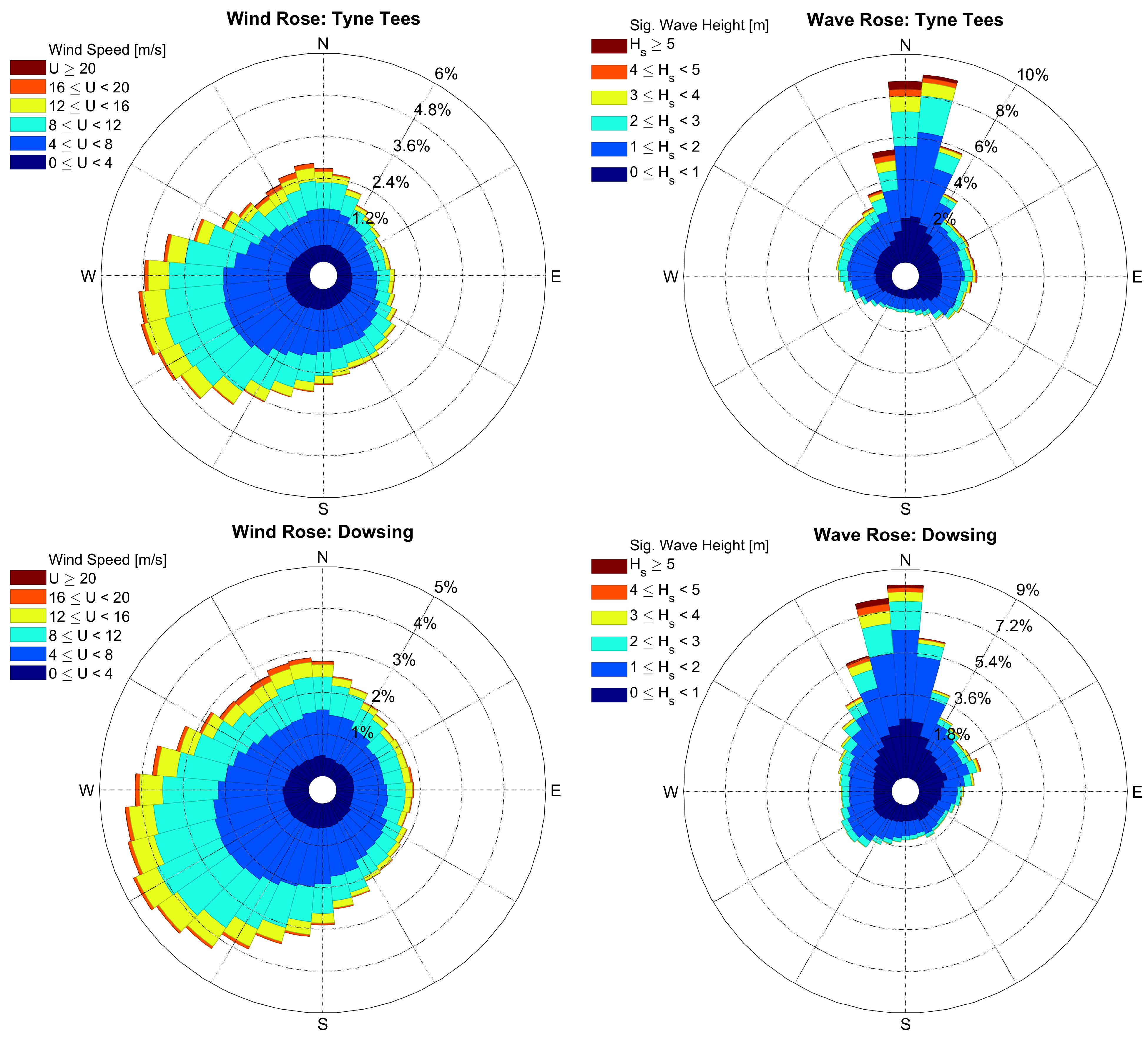
2.1. Observations
2.2. Hindcast Data
3. Methods
3.1. I-FORM
3.2. I-FORM with PCA
3.3. 2D POT
4. Results
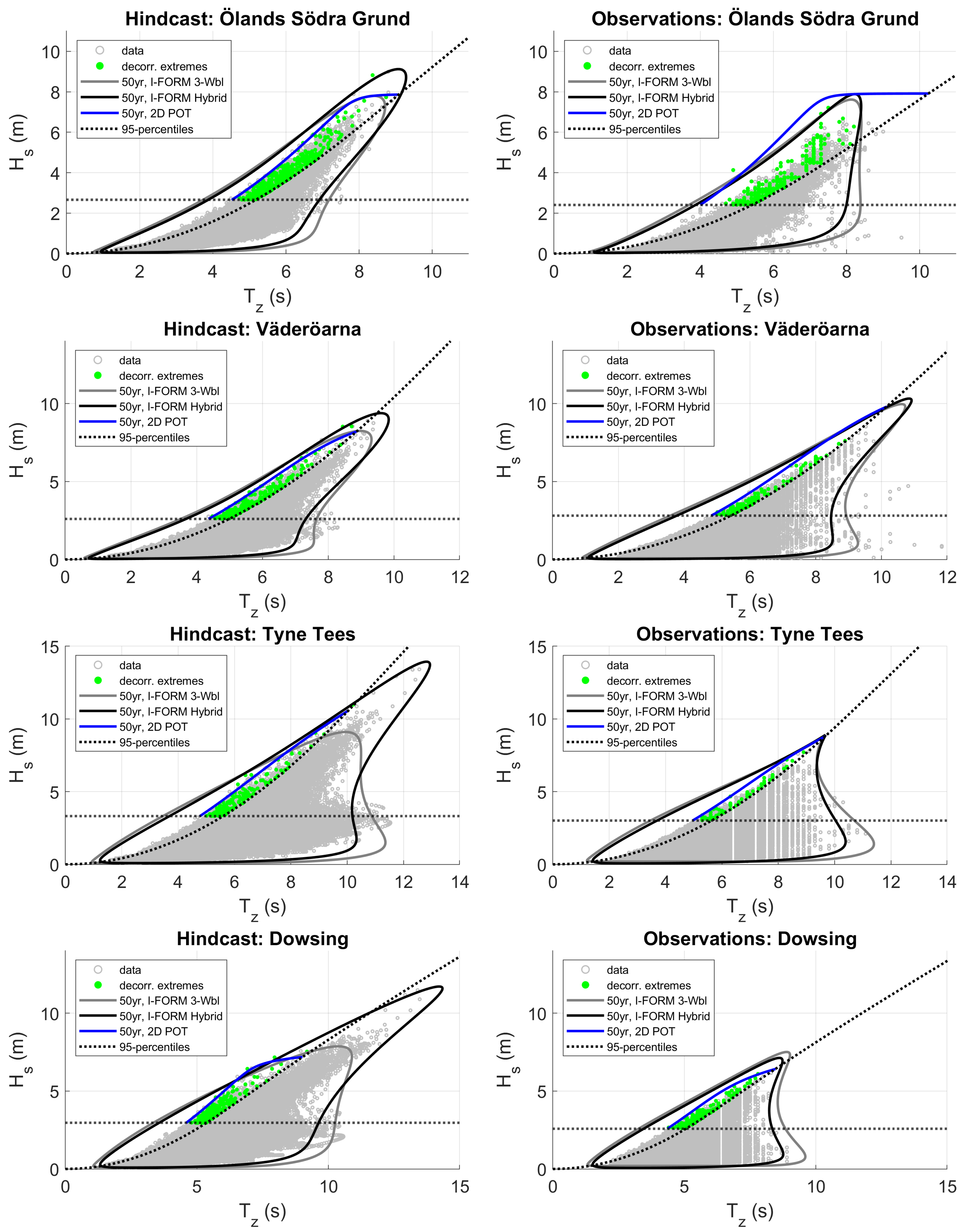
4.1. Implementing Each Method
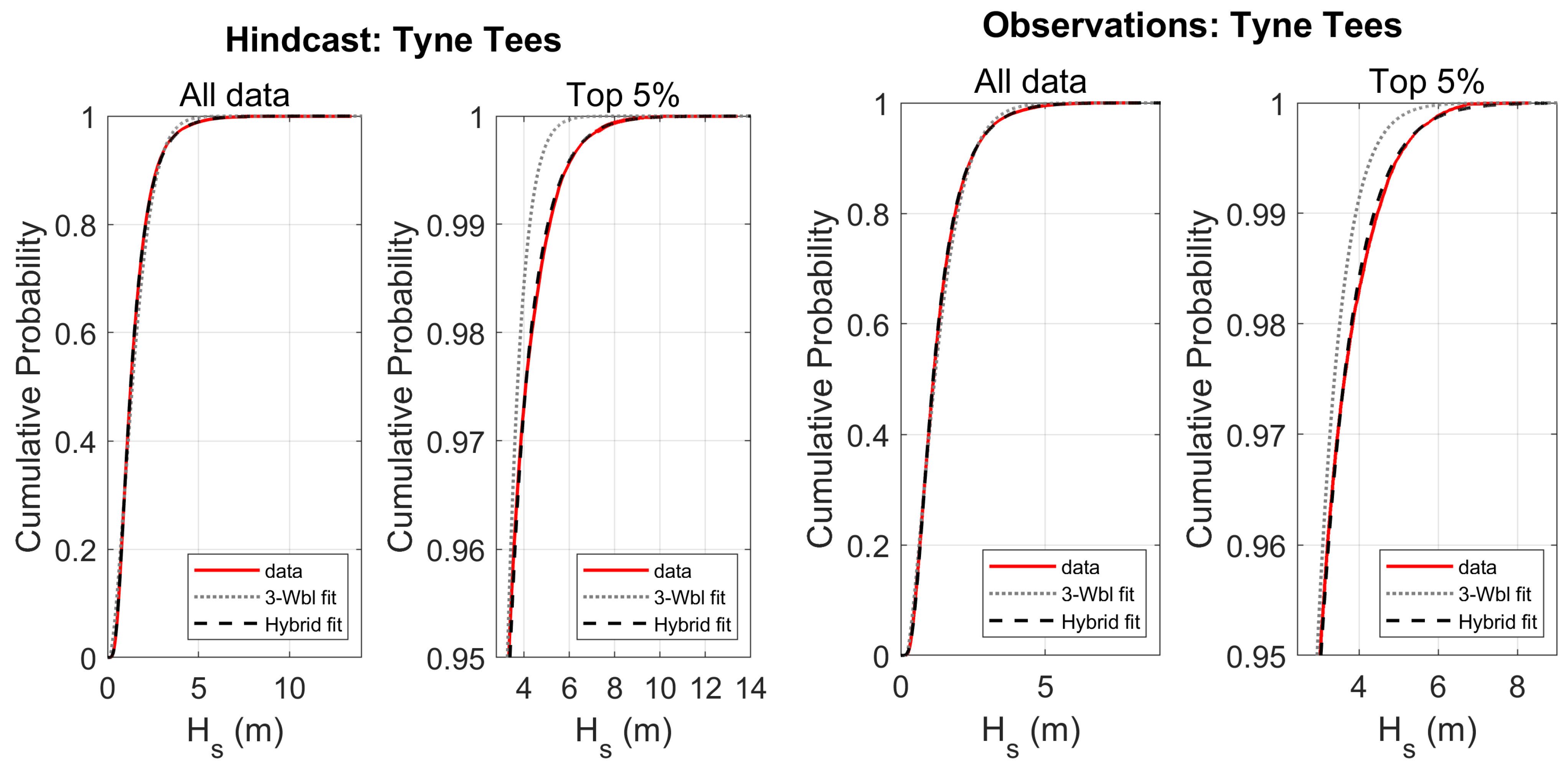
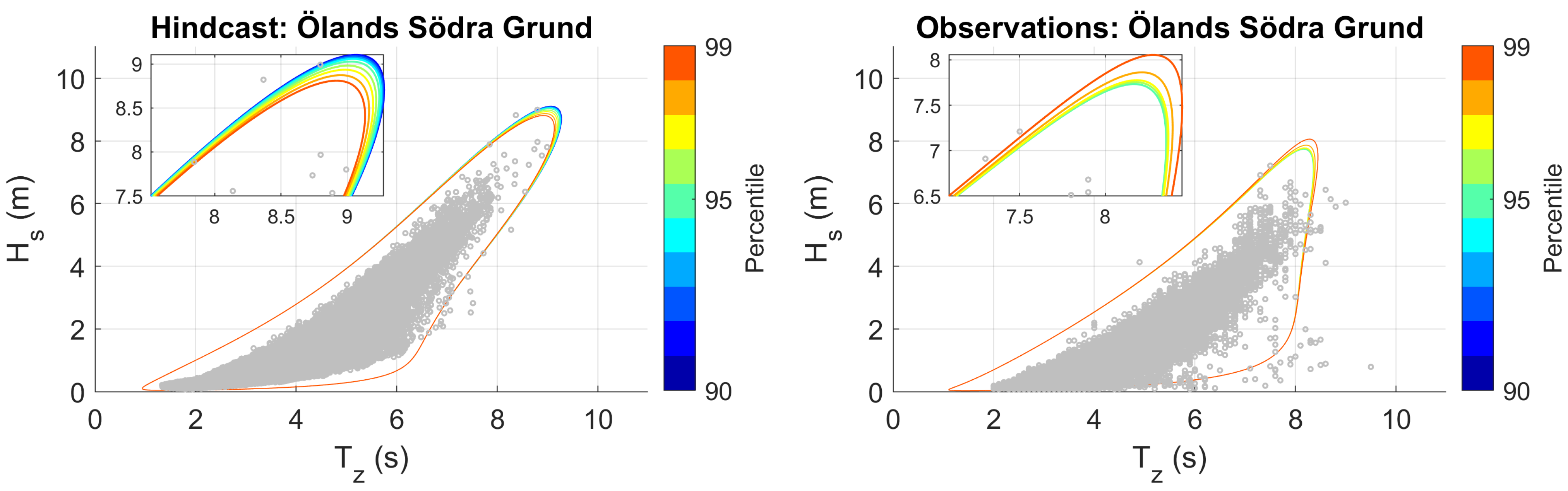
4.1.1. I-FORM
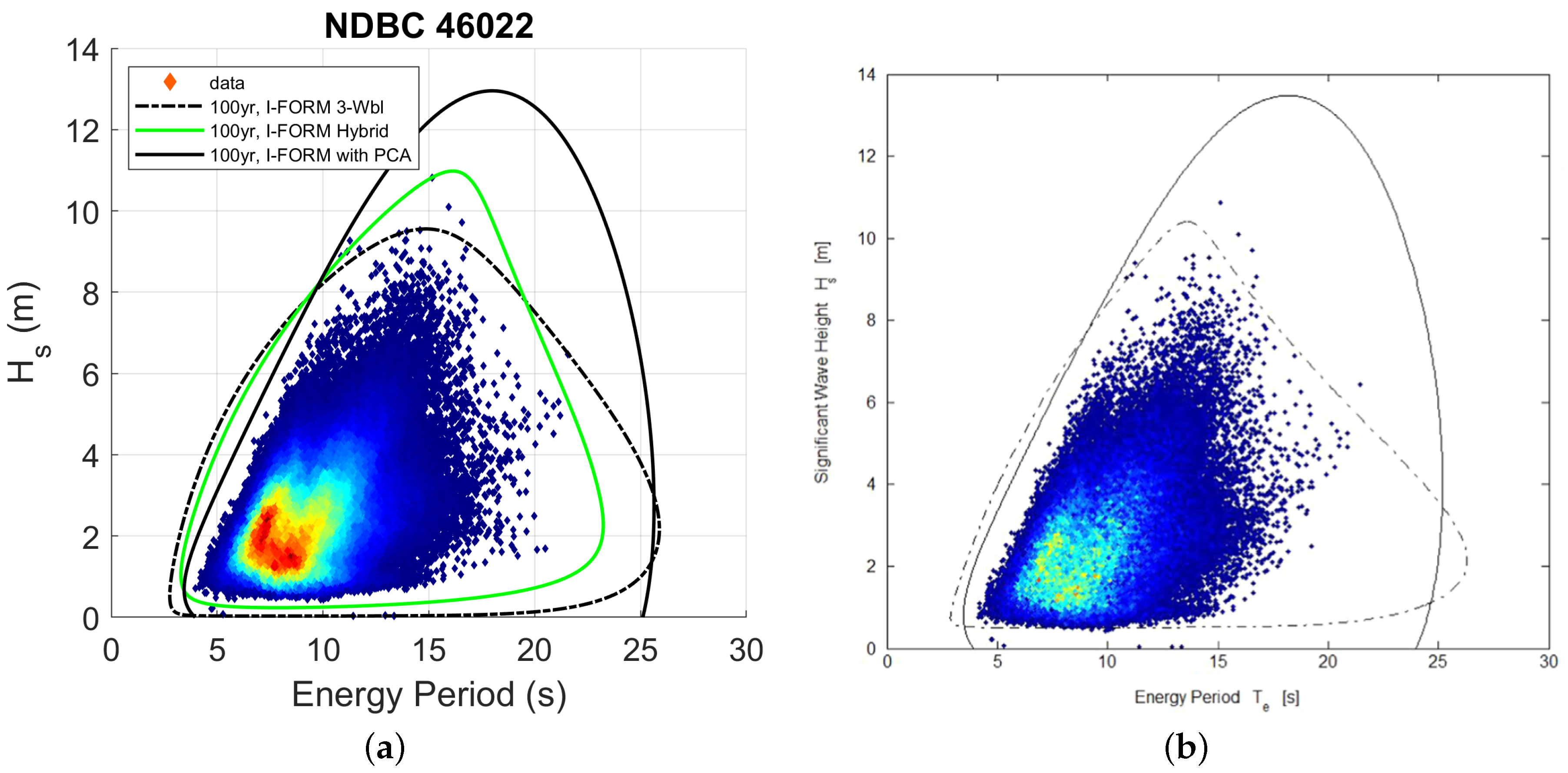
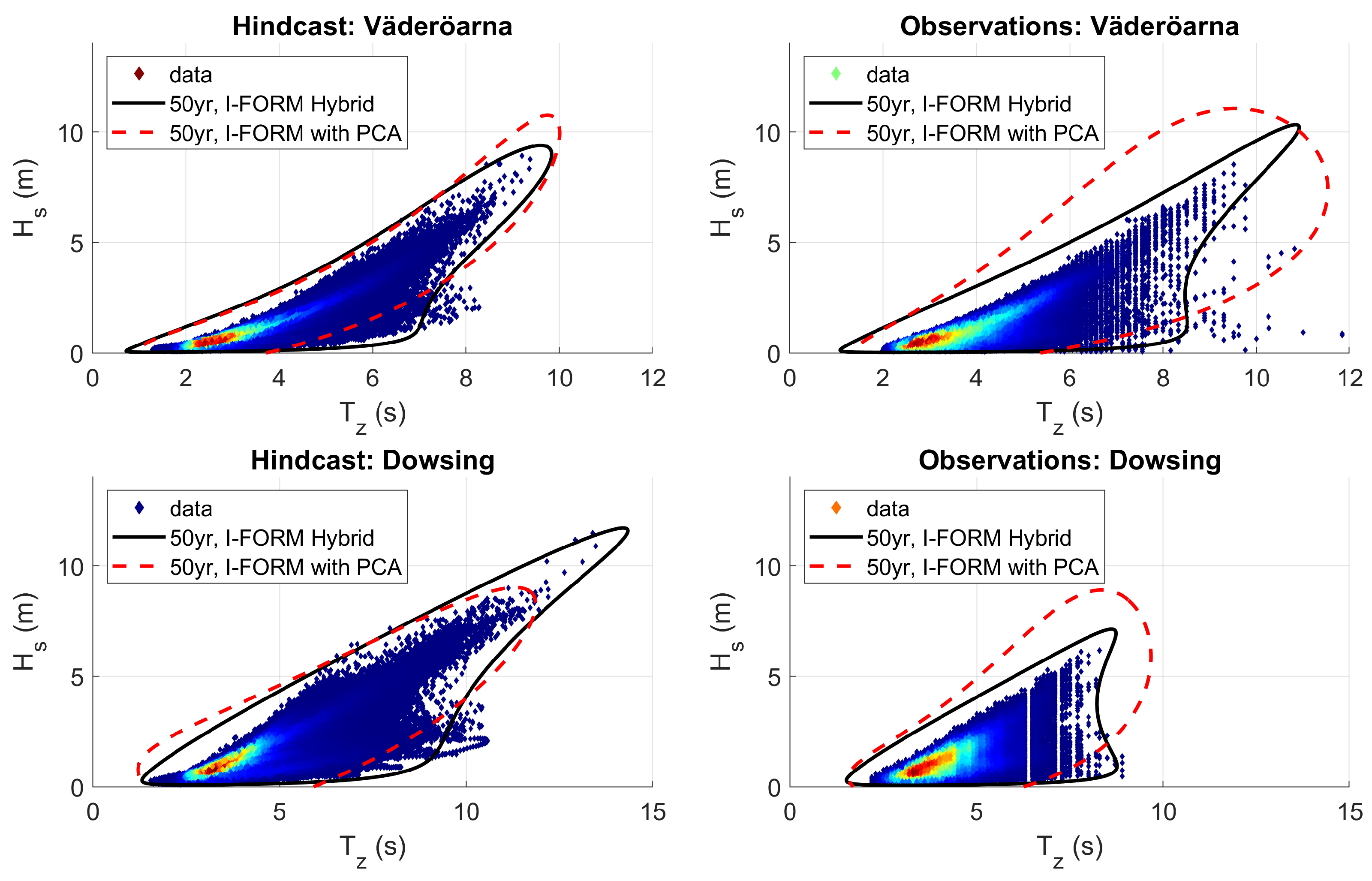
4.1.2. I-FORM with PCA
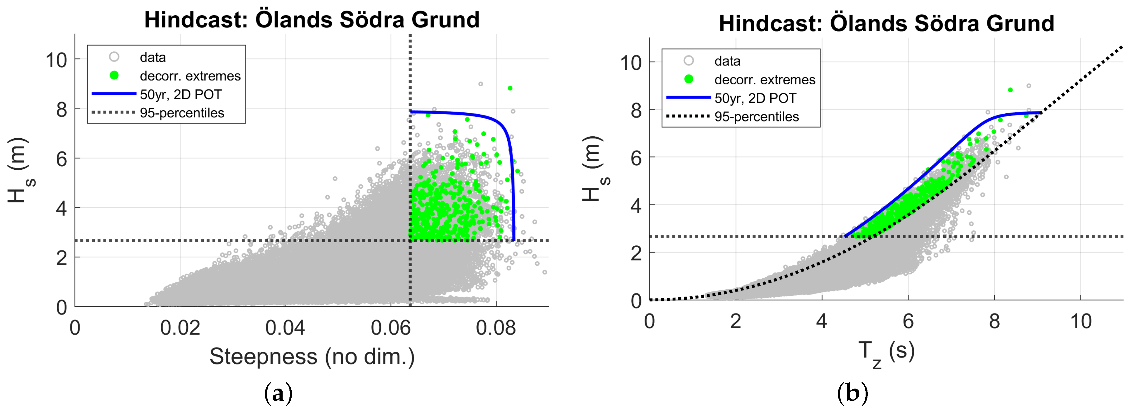
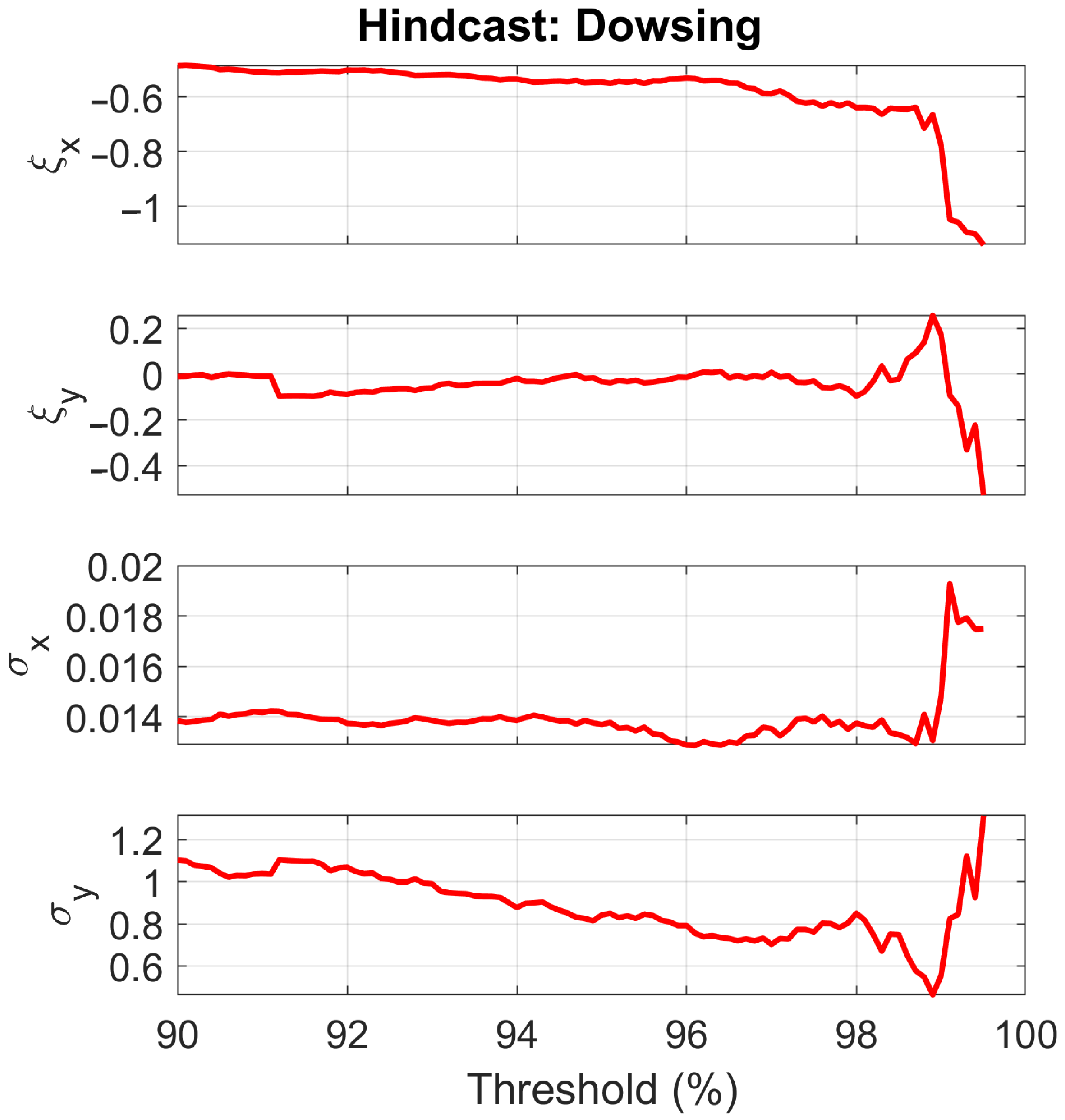
4.1.3. 2D POT
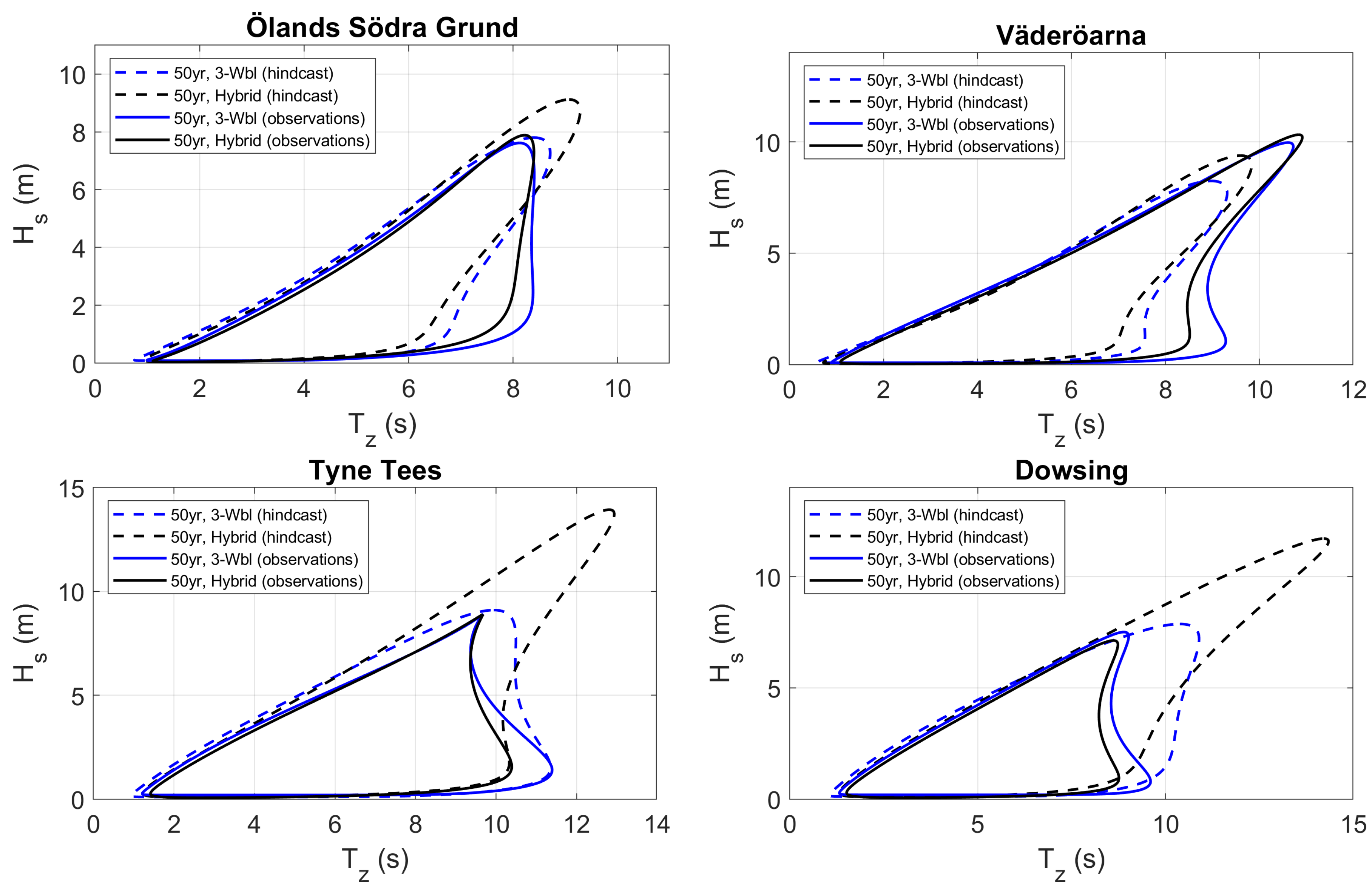
4.2. Comparing the Different Data Sets and Different Methods
5. Discussion
6. Conclusions
Author Contributions
Funding
Institutional Review Board Statement
Informed Consent Statement
Data Availability Statement
Acknowledgments
Conflicts of Interest
References
- Coe, R.G.; Neary, V.S.; Lawson, M.J.; Yu, Y.; Weber, J. Extreme Conditions Modeling Workshop Report; Technical Report; National Renewable Energy Lab.(NREL): Golden, CO, USA, 2014.
- Czech, B.; Bauer, P. Wave Energy Converter Concepts: Design Challenges and Classification. IEEE Ind. Electron. Mag. 2012, 6, 4–16. [Google Scholar] [CrossRef]
- Wolfram, J. On Assessing the Reliability and Availability of Marine Energy Converters: The Problems of a New Technology. Proc. Inst. Mech. Eng. Part O J. Risk Reliab. 2006, 220, 55–68. [Google Scholar] [CrossRef]
- International Electrotechnical Commission. IEC TS 62600-2:2019, Technical Repor. 2019. Available online: https://webstore.iec.ch/publication/62399 (accessed on 12 May 2020).
- NORSOK Standard. Actions and Action Effects, 2nd ed.; Technical Report N-003; Standards Norway: Lysaker, Norway, 2007. [Google Scholar]
- DNV. Environmental conditions and environmental loads. In Recommend Practice DNV-RP-C205; Det Norske Veritas: Hovik, Norway, 2010. [Google Scholar]
- Ransley, E.J. Survivability of Wave Energy Converter and Mooring Coupled System Using CFD. Ph.D. Thesis, Plymouth University, England, UK, 2015. [Google Scholar]
- Yu, Y.H.; van Rij, J.; Coe, R.; Lawson, M. Preliminary Wave Energy Converters Extreme Load Analysis. In Proceedings of the 35th International Conference on Ocean, Offshore and Arctic Engineering (OMAE2015), St. John’s, NL, Canada, 19–24 June 2015. [Google Scholar] [CrossRef]
- Hann, M.; Greaves, D.; Raby, A. Snatch loading of a single taut moored floating wave energy converter due to focussed wave groups. Ocean Eng. 2015, 96, 258–271. [Google Scholar] [CrossRef] [Green Version]
- Göteman, M.; Engström, J.; Eriksson, M.; Leijon, M.; Hann, M.; Ransley, E.; Greaves, D. Wave loads on a point-absorbing wave energy device in extreme waves. J. Ocean Wind Energy 2015, 2, 176–181. [Google Scholar] [CrossRef]
- Coe, R.G.; Neary, V.S. Review of Methods for Modeling Wave Energy Converter Survival in Extreme Sea States. In Proceedings of the 2nd Marine Energy Technology Symposium (METS2014), Seattle, WA, USA, 15–17 April 2014. [Google Scholar]
- Mackay, E. Return Periods of Extreme Loads on Wave Energy Converters. In Proceedings of the 12th European Wave and Tidal Energy Conference, Cork, Ireland, 27 August–1 September 2017. [Google Scholar]
- Hiles, C.E.; Robertson, B.; Buckham, B.J. Extreme wave statistical methods and implications for coastal analyses. Estuar. Coast. Shelf Sci. 2019, 223, 50–60. [Google Scholar] [CrossRef]
- Vanem, E.; Bitner-Gregersen, E.M. Alternative environmental contours for marine structural design-a comparison study. J. Offshore Mech. Arct. Eng. 2015, 137. [Google Scholar] [CrossRef]
- Baarholm, G.S.; Haver, S.; Økland, O.D. Combining contours of significant wave height and peak period with platform response distributions for predicting design response. Mar. Struct. 2010, 23, 147–163. [Google Scholar] [CrossRef]
- Muliawan, M.J.; Gao, Z.; Moan, T. Application of the contour line method for estimating extreme responses in the mooring lines of a two-body floating wave energy converter. J. Offshore Mech. Arct. Eng. 2013, 135, 1–10. [Google Scholar] [CrossRef]
- Rendon, E.A.; Manuel, L. Long-term loads for a monopile-supported offshore wind turbine. Wind Energy 2014, 17, 209–223. [Google Scholar] [CrossRef]
- Coe, R.G.; Yu, Y.H.; Van Rij, J. A Survey of WEC Reliability, Survival and Design Practices. Energies 2018, 11, 4. [Google Scholar] [CrossRef] [Green Version]
- Winterstein, S.R.; Ude, T.C.; Cornell, C.a.; Bjerager, P.; Haver, S. Environmental Parameters for Extreme Response: Inverse Form with Omission Factors. In Proceedings of the Icossar-93, Innsbruck, Austria, 9–13 August 1993; pp. 9–13. [Google Scholar]
- Rosenblatt, M. Remarks on a Multivariate Transformation. Ann. Math. Stat. 1952, 23, 470–472. [Google Scholar] [CrossRef]
- Silva-González, F.; Heredia-Zavoni, E.; Montes-Iturrizaga, R. Development of environmental contours using Nataf distribution model. Ocean Eng. 2013, 58, 27–34. [Google Scholar] [CrossRef]
- Huseby, A.B.; Vanem, E.; Natvig, B. A new approach to environmental contours for ocean engineering applications based on direct Monte Carlo simulations. Ocean Eng. 2013, 60, 124–135. [Google Scholar] [CrossRef]
- Huseby, A.B.; Vanem, E.; Natvig, B. Alternative environmental contours for structural reliability analysis. Struct. Saf. 2015, 54, 32–45. [Google Scholar] [CrossRef]
- Berg, J. Extreme Ocean Wave Conditions for Northern California Wave Energy Conversion Device; SAND Report SAND2011-9034, Technical Report; US Army Corps of Engineers: Washington, DC, USA, 2011.
- Vanem, E. Uncertainties in extreme value modelling of wave data in a climate change perspective. J. Ocean Eng. Mar. Energy 2015, 1, 339–359. [Google Scholar] [CrossRef] [Green Version]
- Haver, S.; Winterstein, S.R. Environmental contour lines: A method for estimating long term extremes by a short term analysis. Trans. Soc. Nav. Archit. Mar. Eng. 2009, 116, 116–127. [Google Scholar]
- Eckert-Gallup, A.C.; Sallaberry, C.J.; Dallman, A.R.; Neary, V.S. Application of principal component analysis (PCA) and improved joint probability distributions to the inverse first-order reliability method (I-FORM) for predicting extreme sea states. Ocean Eng. 2016, 112, 307–319. [Google Scholar] [CrossRef] [Green Version]
- Flocard, F.; Ierodiaconou, D.; Coghlan, I.R. Multi-criteria evaluation of wave energy projects on the south-east Australian coast. Renew. Energy 2016, 99, 80–94. [Google Scholar] [CrossRef]
- Nilsson, E.; Wrang, L.; Rutgersson, A.; Dingwell, A.; Strömstedt, E. Assessment of extreme and metocean conditions in the Swedish exclusive economic zone for wave energy. Atmosphere 2020, 11, 229. [Google Scholar] [CrossRef] [Green Version]
- Neary, V.S.; Ahn, S.; Seng, B.E.; Allahdadi, M.N.; Wang, T.; Yang, Z.; He, R. Characterization of Extreme Wave Conditions for Wave Energy Converter Design and Project Risk Assessment. J. Mar. Sci. Eng. 2020, 8, 289. [Google Scholar] [CrossRef] [Green Version]
- Eckert, A.; Martin, N.; Coe, R.G.; Seng, B.; Stuart, Z.; Morrell, Z. Development of a Comparison Framework for Evaluating Environmental Contours of Extreme Sea States. J. Mar. Sci. Eng. 2021, 9, 16. [Google Scholar] [CrossRef]
- Björkqvist, J.V.; Rikka, S.; Alari, V.; Männik, A.; Tuomi, L.; Pettersson, H. Wave height return periods from combined measurement–model data: A Baltic Sea case study. Nat. Hazards Earth Syst. Sci. 2020, 20, 3593–3609. [Google Scholar] [CrossRef]
- Ross, E.; Astrup, O.C.; Bitner-Gregersen, E.; Bunn, N.; Feld, G.; Gouldby, B.; Huseby, A.; Liu, Y.; Randell, D.; Vanem, E.; et al. On environmental contours for marine and coastal design. Ocean Eng. 2020, 195, 106194. [Google Scholar] [CrossRef]
- Velarde, J.; Vanem, E.; Kramhøft, C.; Sørensen, J.D. Probabilistic analysis of offshore wind turbines under extreme resonant response: Application of environmental contour method. Appl. Ocean Res. 2019, 93, 101947. [Google Scholar] [CrossRef]
- Björkqvist, J.V.; Lukas, I.; Alari, V.; van Vledder, G.P.; Hulst, S.; Pettersson, H.; Behrens, A.; Männik, A. Comparing a 41-year model hindcast with decades of wave measurements from the Baltic Sea. Ocean Eng. 2018, 152, 57–71. [Google Scholar] [CrossRef] [Green Version]
- Weisse, R.; Gaslikova, L.; Geyer, B.; Groll, N.; Meyer, E. coastDat—Model Data for Science and Industry. Die Küste 81 Model. 2014, 81, 5–18. [Google Scholar]
- Weisse, R. coastDat-1 Waves Baltic Sea; World Data Center for Climate (WDCC) at DKRZ: Hamburg, Germany, 2015. [Google Scholar] [CrossRef]
- Weisse, R. coastDat-1 Waves North Sea Wave Spectra Hindcast (1948–2007); Helmholtz-Zentrum Geesthacht, Zentrum für Material- und Küstenforschung GmbH: Geesthacht, Germany; World Data Center for Climate (WDCC) at DKRZ: Hamburg, Germany, 2012. [Google Scholar] [CrossRef]
- Kalnay, E.; Kanamitsu, M.; Kistler, R.; Collins, W.; Deaven, D.; Gandin, L.; Iredell, M.; Saha, S.; White, G.; Woollen, J.; et al. The NCEP/NCAR 40-year reanalysis project. Bull. Am. Meteorol. Soc. 1996, 77, 437–471. [Google Scholar] [CrossRef] [Green Version]
- Jacob, D.; Podzun, R. Sensitivity studies with the regional climate model REMO. Meteorol. Atmos. Phys. 1997, 63, 119–129. [Google Scholar] [CrossRef]
- The Wamdi Group. The WAM model—A third generation ocean wave prediction model. J. Phys. Oceanogr. 1988, 18, 1775–1810. [Google Scholar] [CrossRef] [Green Version]
- Holthuijsen, L.H. Waves in Oceanic and Coastal Waters; Cambridge University Press: New York, NY, USA, 2007; p. 387. [Google Scholar] [CrossRef]
- Sheng, W.; Li, H. A method for energy and resource assessment of waves in finite water depths. Energies 2017, 10, 460. [Google Scholar] [CrossRef] [Green Version]
- Shanas, P.R.; Kumar, V.S. Trends in surface wind speed and significant wave height as revealed by ERA-Interim wind wave hindcast in the Central Bay of Bengal. Int. J. Climatol. 2015, 35, 2654–2663. [Google Scholar] [CrossRef]
- Bengtsson, L.; Hagemann, S.; Hodges, K.I. Can climate trends be calculated from reanalysis data? J. Geophys. Res. D Atmos. 2004, 109. [Google Scholar] [CrossRef] [Green Version]
- Semedo, A. Seasonal variability of wind sea and swell waves climate along the Canary Current: The local wind effect. J. Mar. Sci. Eng. 2018, 6, 28. [Google Scholar] [CrossRef] [Green Version]
- Nadarajah, S.; Cordeiro, G.M.; Ortega, E.M. The exponentiated Weibull distribution: A survey. Stat. Pap. 2013, 54, 839–877. [Google Scholar] [CrossRef]
- Chang, K.H. Reliability Analysis. In e-Design Computer-Aided Engineering Design; Chang, K.H., Ed.; Academic Press: Boston, MA, USA, 2015; Chapter 10; pp. 523–595. [Google Scholar] [CrossRef]
- Haver, S.; Nyhus, K.A. A wave climate description for long term response calculations. In Proceedings of the OMAE’1986, Tokyo, Japan, 13–18 April 1986. [Google Scholar]
- Haver, S. On the Prediction of Extreme Wave Crest Heights; Technical Report; Manuscript, Statoil: Stavanger, Norway, 2004. [Google Scholar]
- Laio, F. Cramer-von Mises and Anderson-Darling goodness of fit tests for extreme value distributions with unknown parameters. Water Resour. Res. 2004, 40. [Google Scholar] [CrossRef]
- Mazas, F.; Hamm, L. An event-based approach for extreme joint probabilities of waves and sea levels. Coast. Eng. 2017, 122, 44–59. [Google Scholar] [CrossRef]
- Simarro, G.; Orfila, A. Improved explicit approximation of linear dispersion relationship for gravity waves: Another discussion. Coast. Eng. 2013, 80, 15. [Google Scholar] [CrossRef]
- Beji, S. Improved explicit approximation of linear dispersion relationship for gravity waves. Coast. Eng. 2013, 73, 11–12. [Google Scholar] [CrossRef]
- Coles, S. An Introduction to Statistical Modeling of Extreme Values; Springer Series in Statistics; Springer: London, UK, 2001. [Google Scholar] [CrossRef]
- De Oliveira, M.M.F.; Ebecken, N.F.F.; de Oliveira, J.L.F.; Gilleland, E. Generalized extreme wind speed distributions in South America over the Atlantic Ocean region. Theor. Appl. Climatol. 2011, 104, 377–385. [Google Scholar] [CrossRef] [Green Version]
- Aarnes, O.J.; Breivik, Ø.; Reistad, M. Wave Extremes in the northeast Atlantic. J. Clim. 2012, 26. [Google Scholar] [CrossRef] [Green Version]
- Bevacqua, E.; Maraun, D.; Vousdoukas, M.I.; Voukouvalas, E.; Vrac, M.; Mentaschi, L.; Widmann, M. Higher probability of compound flooding from precipitation and storm surge in Europe under anthropogenic climate change. Sci. Adv. 2019, 5. [Google Scholar] [CrossRef] [PubMed] [Green Version]
- Serinaldi, F. Dismissing return periods! Stoch. Environ. Res. Risk Assess. 2015, 29, 1179–1189. [Google Scholar] [CrossRef] [Green Version]
- Haselsteiner, A.F.; Ohlendorf, J.H.; Wosniok, W.; Thoben, K.D. Deriving environmental contours from highest density regions. Coast. Eng. 2017, 123, 42–51. [Google Scholar] [CrossRef]
- National Data Buoy Center. Station 46022 (LLNR 500)—Eel River—17NM WSW of Eureka, CA. 2020. Available online: https://www.ndbc.noaa.gov/station_page.php?station=46022 (accessed on 18 May 2020).
- Webber, J.B.W. A bi-symmetric log transformation for wide-range data. Meas. Sci. Technol. 2013, 24. [Google Scholar] [CrossRef] [Green Version]
- Parker, K.; Hill, D.F. Evaluation of bias correction methods for wave modeling output. Ocean Model. 2017, 110, 52–65. [Google Scholar] [CrossRef]
- AghaKouchak, A.; Easterling, D.; Hsu, K.; Schubert, S.; Sorooshian, S. Extremes in a Changing Climate: Detection, Analysis and Uncertainty; Springer: Dordrecht, The Netherlands, 2012; p. 429. [Google Scholar]
- Woo, H.J.; Park, K.A. Long-term trend of satellite-observed significant wave height and impact on ecosystem in the East/Japan Sea. Deep Sea Res. Part II Top. Stud. Oceanogr. 2017, 143, 1–14. [Google Scholar] [CrossRef]
- Caloiero, T.; Aristodemo, F.; Algieri Ferraro, D. Trend analysis of significant wave height and energy period in southern Italy. Theor. Appl. Climatol. 2019, 138, 917–930. [Google Scholar] [CrossRef]
- Eckert-Gallup, A.; Martin, N. Kernel density estimation (KDE) with adaptive bandwidth selection for environmental contours of extreme sea states. In Proceedings of the OCEANS 2016 MTS/IEEE Monterey, OCE 2016, Monterey, CA, USA, 19–23 September 2016. [Google Scholar] [CrossRef]
- Hao, Z.; Singh, V.P.; Hao, F. Compound extremes in hydroclimatology: A review. Water 2018, 10, 718. [Google Scholar] [CrossRef] [Green Version]
- Owusu, P.A.; Asumadu-Sarkodie, S. A review of renewable energy sources, sustainability issues and climate change mitigation. Cogent Eng. 2016, 3. [Google Scholar] [CrossRef]


| Site | Lat | Lon | Depth [m] | Distance [km] | (obs.) [m] | (hind.) [m] | Availability [years] |
|---|---|---|---|---|---|---|---|
| Ölands Södra Grund | 56.0667° N | 16.6833° E | 38 | 22 | 1.03 | 1.09 | 16.7 |
| Väderöarna | 58.4833° N | 10.9333° E | 72 | 18 | 1.12 | 1.05 | 12.6 |
| Tyne Tees | 54.9190° N | 0.7487° W | 66 | 37 | 1.34 | 1.51 | 10.8 |
| Dowsing | 53.5318° N | 1.0538° E | 22 | 56 | 1.23 | 1.36 | 15.4 |
| Max Hs (m) | Cond. max s | ||||
|---|---|---|---|---|---|
| Site | Data | 3-Wbl | Hybrid | 3-Wbl | Hybrid |
| Ölands Södra Grund | obs. hind. | 7.61 7.80 | 7.88 9.12 | 0.099 0.109 | 0.093 0.103 |
| Väderöarna | obs. hind. | 9.97 8.25 | 10.32 9.38 | 0.105 0.104 | 0.098 0.099 |
| Tyne Tees | obs. hind. | 9.07 9.10 | 10.58 13.94 | 0.121 0.147 | 0.112 0.133 |
| Dowsing | obs. hind. | 7.51 7.87 | 7.13 11.71 | 0.138 0.164 | 0.125 0.145 |
Publisher’s Note: MDPI stays neutral with regard to jurisdictional claims in published maps and institutional affiliations. |
© 2021 by the authors. Licensee MDPI, Basel, Switzerland. This article is an open access article distributed under the terms and conditions of the Creative Commons Attribution (CC BY) license (http://creativecommons.org/licenses/by/4.0/).
Share and Cite
Wrang, L.; Katsidoniotaki, E.; Nilsson, E.; Rutgersson, A.; Rydén, J.; Göteman, M. Comparative Analysis of Environmental Contour Approaches to Estimating Extreme Waves for Offshore Installations for the Baltic Sea and the North Sea. J. Mar. Sci. Eng. 2021, 9, 96. https://0-doi-org.brum.beds.ac.uk/10.3390/jmse9010096
Wrang L, Katsidoniotaki E, Nilsson E, Rutgersson A, Rydén J, Göteman M. Comparative Analysis of Environmental Contour Approaches to Estimating Extreme Waves for Offshore Installations for the Baltic Sea and the North Sea. Journal of Marine Science and Engineering. 2021; 9(1):96. https://0-doi-org.brum.beds.ac.uk/10.3390/jmse9010096
Chicago/Turabian StyleWrang, Linus, Eirini Katsidoniotaki, Erik Nilsson, Anna Rutgersson, Jesper Rydén, and Malin Göteman. 2021. "Comparative Analysis of Environmental Contour Approaches to Estimating Extreme Waves for Offshore Installations for the Baltic Sea and the North Sea" Journal of Marine Science and Engineering 9, no. 1: 96. https://0-doi-org.brum.beds.ac.uk/10.3390/jmse9010096