A Novel Profiler Driven by Tidal Energy for Long Term Oceanographic Measurements in Offshore Areas

Abstract

In this paper, an innovative profiler driven by tidal energy for long-term oceanographic measurements in offshore areas with abundant tidal resources is investigated. The profiler is mainly composed of an oceanographic data collection system equipped with various sensors and a cross-plate that can make an upward or downward movement under the impact of tidal currents. Theoretical research is carried out through static analysis and numerical simulation, mainly studying the hydrodynamic characteristics of the cross-plate and its dynamic response to the current velocity. The theoretical model is verified by comparison with experiments. The research results show that tidal energy can be used as a kind of energy to drive the profiler’s ascent and descent motion and to continuously measure ocean parameters without using electric energy. The theoretical model established in this study can roughly predict the position of the profiler observation platform in the vertical direction under various current velocities. Furthermore, by studying the relationship between the current velocities and the lift and drag forces of the cross-plate in the fluid, it is recognized that the current velocity is an important factor affecting the stability of the system’s motion. It is hoped that this research will contribute to the development of profilers.

1. Introduction

Monitoring the oceans is an activity of primary importance, not only for ongoing research related to weather forecasting, seasonal and climate prediction, but also for other activities such as marine environmental protection, fisheries management, and maritime safety [1]. It has been well recognized that the long-term, autonomous, reliable and affordable vertical profile measurements of seawater parameters in specific areas highly contribute to oceanographic research, climate prediction, and disaster prevention. So far there have been many observational instruments and devices for measuring profiles of ocean properties over long periods.

There has been a considerable amount of studies on ocean profile measurement methods over the past decades. Two traditional ways are used to measure marine profile parameters. One of the methods is to use ship-borne devices of most oceanographic vessels. However, these onboard instruments require winches to complete the measurements, which is fairly labor-intensive and requires a staggering amount of financial resources. Another method is to use self-contained instruments mounted on oceanographic moorings. Data collected by this method, for the most part, is discrete. To improve the sampling density, multiple sensors need to be laid in layers along the mooring, which will increase equipment costs and lead to the complexity of the whole mooring system, and further have an impact on field operation.

However, it has been found that the two methods above will be unsustainable in the long run as they are highly restrictive in space and time coverage and prohibitively expensive [2]. Various autonomous profiling platforms have been developed and pervasively used to address the issue without keeping a ship on station for long periods.

The Argo Program is a major component of both the Global Ocean Observing System (GOOS) and the Global Climate Observing System (GCOS) [3,4]. A key objective of Argo is to observe oceanic signals related to climate change. Argo systems use battery packs as the power plant. The drive motor controls the piston to move back and forth to change the volume of a rubber bladder, which causes a change in the relationship between buoyancy and gravity, further moving the platform up and down. The Argo Program has provided global coverage of the upper 2000 m of the oceans since 2006. By November 2018, Argo had obtained 2,000,000 profiles since the program began its implementation in 1999 [5]. MRVP [6], ALACE [7], PROVOR [8], YOYO [9], and Automatic Profiling System made by the Russian Academy of Sciences [10] work the same principle as Argo, all based on Archimedes’ law.

Wilson et al. designed an AMP (Autonomous Moored Profiler) tethered to an anchor by a winch system, which is designed to monitor water quality applications in depths less than 50 m at a fixed geographical location [11]. A 1.5 kWh battery pack is used as the power plant to run the AMP. During July and August 2010, AMP was deployed on the east slope of the Chesapeake Bay “Deep Channel”. Before the AMP is studied, the Miniaturized Autonomous Moored Profiler (Mini AMP) designed by WET Labs includes a robust suite of physical, biological, and optical sensors, an integrated package control system, a power system, and a telemetry unit as a part of a modular, winch-driven profiling platform to meet naval needs [11,12].

MRL (The McLane Research Laboratories, Inc.) and WHOI (the Woods Hole Oceanographic Institution) of Massachusetts, USA collaborated to complete the development of the McLane Moored Profiler (MMP) [13]. The proven features and technology of the WHOI Moored Profiler were incorporated into the new design [14]. The along-cable speed of MMP is about 25 cm/s when the nominal voltage of the lithium battery pack is 10.8 V [15]. The roller rotates counterclockwise or clockwise under the control of the precious metal brush DC motor and then drives the platform to move up and down along the guide cable [16]. The University of Washington Applied Physics Lab (APL) installed a Deep Profiler System that included a modified MMP equipped with the rechargeable battery pack which used the inductive coupling charging technique to charge the MMP [17]. The profiler similar to MMP is the Russian Aqualog, which has been deployed in sea trials in many sea areas around the world, such as the Black Sea, Red Sea, and Red Sea, and has achieved small batch production [18].

However, the power-driven source of all the profilers mentioned above comes from the battery pack which is scarce in marine vehicles. As the battery is sensitive to short circuit, corrosion, pressure, and other maladies, it must be sealed in a cabin made of stainless steel, titanium alloy, or other materials with a density far greater than that of seawater, which adds weight and structural complexity to the entire platform. To handle these issues, types of profilers without using electric energy have been researched.

Ocean University of China designed a potential-energy-driven reciprocating ocean profiler (PedROP) prototype with SBE37 CTD [19]. The system uses a design method that separates the driving unit and the observation unit. The power-driven unit drops only one steel ball into the observation unit at a time. When the steel ball enters the observation unit, the gravity of the observation unit is greater than the buoyancy, thereby realizing the descending motion. When the observation unit moves and hits the bottom stopper, the steel ball is thrown out, and the buoyancy of the observation unit is greater than gravity, thereby realizing the ascending movement. Each steel ball can provide a reciprocating power, so the multiple steel balls stored in the power-driven unit can provide power to the observation unit for multiple reciprocating motions. The prototype has been tested in the South China Sea for 5 days, and 11 CTD data of reciprocating profiles have been obtained. The length of each section is 1000 m, and the reciprocating velocity of the platform reaches 0.3 m/s.

The State Key Lab of Fluid Power Transmission and Control of Zhejiang University uses the phase change material (PCM) to absorb and release the temperature difference energy that is further converted to mechanical energy and drive the vertical action of the profiler [20].

Scripps Institute of Oceanography designed the Wirewalker (WW) which is a vertically profiling instrument package propelled by ocean waves [21]. The elements of the WW system include a surface buoy, a wire suspended from the buoy, a weight at the end of the wire, and the profiler itself. The relative motion between the wire and the water is used to propel the Wirewalker profiler. Prototypes of Wirewalker systems have been deployed in the North Pacific, Indian Oceans, and elsewhere. The Wirewalker profiles 1000–3000 km month⁻¹, vertically, with typical missions lasting from days to months. The Seahorse vertical profiler developed by the Bedford Institute of Oceanography is a high-tech predecessor of the Wirewalker [22].

The Autonomous Ocean Profiler (AOP) is an oceanographic instrument platform based on a current-drive, which can be used to measure profiles of physical, thermodynamic, and biological properties in the Arctic Ocean. The hydrodynamic lift of the platform is produced when the prevailing currents hit the delta wing. When the current speed is as low as 3 cm/s, AOP can still traverse the cable [23,24]. A series of tests of AOP operation were conducted in Puget Sound in water depths between 150 and 200 m [23,24].

For the above four profilers, the profiler using ocean temperature difference energy has no physical prototype, and has not been verified by sea trial; AOP not only uses tidal energy as a driving energy, but also uses electrical energy to control the pitch of its wings; PedROP and Wirewalker move up and down along the rope, so when the tidal current velocity is high, the stability of the entire system will be affected to a certain extent.

Table 1. Typical representatives of profilers and their characteristics.

Typical Representatives of Profiler	Energy Source	Maximum Deployment Depth (Meters)	Sea Trial Deployment	Similar Equipments
ARGO	electricity	6000	global ocean areas	ALACE, MRVP, PROVOR, YOYO, et al.
AMP	electricity	<50	the Chesapeake Bay	Mini AMP, the Profiling Buoy of NGK
MMP	electricity	30~6000	the Labrador and Weddell Seas	WHOI Moored Profiler, Aqualog
Wirewalker	wave energy	300	the North Pacific	Seahorse
AOP	currents and electricity	150~200	the Arctic Ocean	/
PedROP	gravitational potential energy	300~1300	the South China Sea	/
Ocean Profiler Power System of ZJU	temperature difference energy	60	/	/

simply summarizes the characteristics of all the profilers mentioned above. Tides are the vertical movement of the oceans and seas caused by the rotation of the earth and the relative movements of the earth, moon, sun, and to a much lesser extent, other celestial bodies. Tidal currents are totally quantifiable and predictable spatially and temporally strictly speaking [25]. Nowadays, increased attention is being given to tidal current energy development all over the world [26]. Tidal currents are a hopeful candidate for renewable energy in the ocean environment.

The main objective of this study is to propose a new profiler driven by tidal currents, to avoid technical difficulties and inconveniences brought by battery packs. Utilizing tidal current energy for repeated ascent and descent of the oceanographic instrument greatly extends unattended operation, which is beneficial to develop efficient, reliable, and low-cost platforms to provide oceanographic data over long periods. While being deployed in areas with periodic tidal currents, data in different water depths can be obtained by adjusting sampling time. Because the upper mooring buoy is relatively far from the sea surface, this article will not study the influence of waves on the performance of the instrument. We theoretically analyzed the vertical movement range of this equipment in seawater. The flume experiments are used to test the validity of the theoretical model.

The outline of this paper is as follows. The theoretical model is outlined in Section 2, together with the working principle of the system, the static analysis, and numerical simulations. The setup and method of the flume experiments and the deployment of the system are introduced in Section 3. In Section 4, the theoretical results obtained by simulation and mechanical calculations are compared with the results of the flume experiments. Some results are presented, mainly including the vertical motion range of the profiler and the effect of current velocity on system motion stability. Some conclusions are given in Section 5.

2. Theoretical Model

2.1. Working Principle of the System

When the kinetic energy in a moving fluid is converted into the motion of the mechanical system, the energy in the tide flow is used [27].

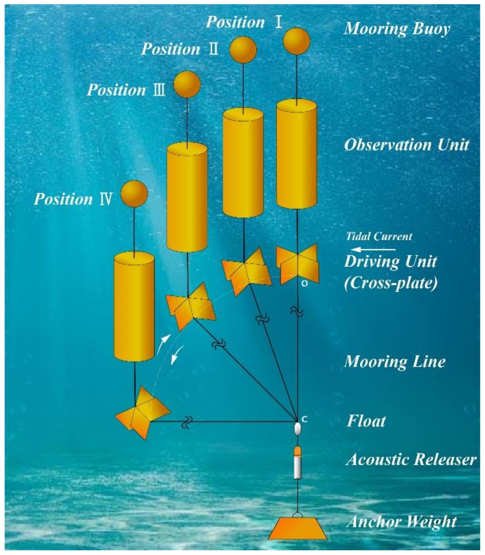
Figure 1 physically describes the mechanism of the profiler. The profiler is mainly composed of three parts: the driving unit, the observation unit, and the mooring system. The cross-plate is composed of two mutually perpendicular cross-plates, as the driving unit of the entire platform, will swing around a certain point affected by the tidal current. At the same time, the swing mechanism of the cross-plate is suitable for alternating stream directions of tidal current. The tilt angle of the cross-plate axis is passively adjustable to the current velocity. The buoyancy of the system will be adjusted to offset its weight in water. Ideally, when the current velocity approaches zero, the cross-plate is almost perpendicular to the sea level, and the driving unit is at the highest point, as in position I in the figure. Since the tidal current will exert a force on the cross-plate, and the distance between points O and C is fixed, the cross-plate will deviate from the vertical position and gradually rotate counterclockwise. If the current velocity is large enough and the cross-plate is appropriately designed, the cross-plate will eventually rotate close to the bottom of the sea, as shown in position IV. The observation unit will follow the driving unit down to the lowest point under the traction of the mooring cable. Conversely, if the tidal current velocity slows down to zero, the driving unit will rotate clockwise to its original position. Then, the driving unit will move to the highest point again. Therefore, the observation unit can move up and down, and the instruments and sensors mounted on it can sample vertically and continuously within a certain depth range. In this process, the kinetic energy of the tidal current is converted into the reciprocating motion of the platform.

To determine the range of motion of the cross-plate in the vertical direction, it is necessary to calculate its position, which means that the dynamic analysis of the system is very important.

2.2. Static Analysis of the Model

A plate at the incidence of less than 90° will have a tangential force acting on it due to skin friction. However, the tangential force is not significant compared with the normal force except at incidences below about 10°. So the tangential force will be neglected in our research.

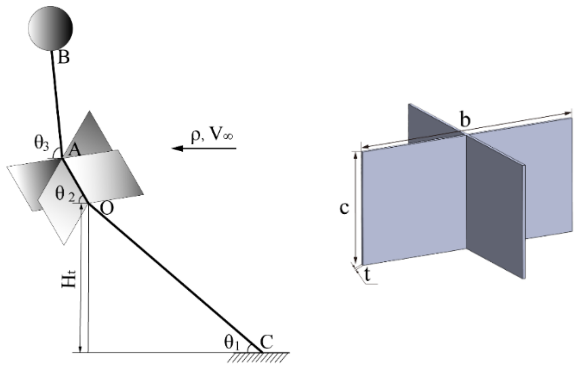
Since the position of the observation platform will change up and down with the position of the cross-plate, the key to the theoretical calculation of this system is to calculate the position of the cross-plate. Therefore, the following theoretical calculation will temporarily remove the observation platform and indirectly calculate the position of the cross-plate by calculating the ${\theta }_{1,}$ ${\theta }_2$ and ${\theta }_3$ in Figure 2 that shows the environment and geometric parameters of the system.

As shown in Figure 2, the length of the rope between point A and B is $L_{AB},$ and the length of the rope between point O and C is $L_{oc}.$ The vertical distance in theory between point O and point C is $H_t$. The angle between the rope AB connecting the buoy to the cross-plate and the horizontal plane is ${\theta }_3$. The angle between the cross-plate and the horizontal plane is ${\theta }_2$. The angle between the rope OC connecting the cross-plate to the anchor and the horizontal plane is ${\theta }_1$. The span of the cross-plate is b, the chord of it is c, and the thickness is t. The buoy is a hollow spherical shell with an outer diameter of ${\mathrm{R}}_o$ and an inner diameter of ${\mathrm{R}}_i$. The buoy mass is ${\mathrm{m}}_q$. $V_{\infty }$ represents the approach velocity of the horizontal current. The fluid density is $\rho$.

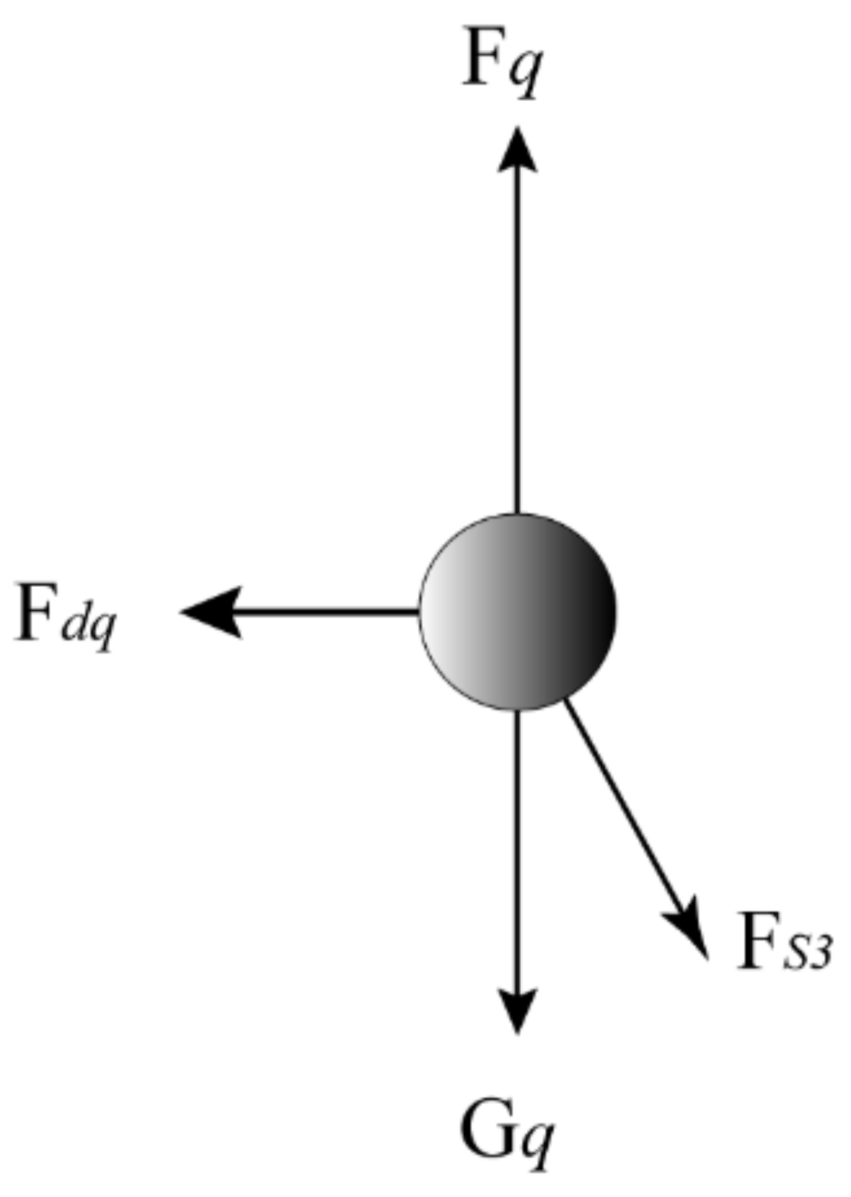
Figure 3 shows the force analysis of the buoy, where $F_q$ and $G_q$ are the buoy’s buoyancy and gravity, $F_{dq}$ is the drag of the buoy in the flow field, and $F_{s3}$ is the rope’s pull on the buoy.$F_q$, $G_q$ and $F_{dq}$ can be calculated by Equations (1)–(3), respectively, where $F_q$ and $G_q$ are the buoy’s buoyancy and gravity, $F_{dq}$ is the drag of the buoy in the flow field, and $F_{s3}$ is the rope’s pull on the buoy.$F_q$, $G_q$ and $F_{dq}$ can be calculated by Equations (1)–(3), respectively.

$$F_q=\frac{4}{3}\rho g\pi R_o{}^3$$

(1)

$$G_q=m_{q}g$$

(2)

$$F_{dq}=\frac{1}{2}{C}_{dq}\rho V_{\infty }{}^2\pi R_o{}^2$$

(3)

where $C_{dq}$ is the drag coefficient of the buoy, and it is relatively steady in the range of Reynolds number between about ${10}^3$ and $2\times {10}^5$. The Reynolds number in this study is less than ${10}^5$ and greater than ${10}^3$, so the value of $C_{dq}$ is taken as a constant 0.47 [28].

In the horizontal direction and vertical direction, the force balance formula of the buoy is shown in Equations (4) and (5).

$$F_{dq}=F_{s3}\cos {\theta }_3$$

(4)

$$F_q=G_q+F_{s3}\sin {\theta }_3$$

(5)

Solving Equations (4) and (5),${\theta }_3$ and $F_{s3}$ can be expressed by Equations (6) and (7), respectively.

$${\theta }_3=\arctan \left(\frac{F_q-G_q}{F_{dq}}\right)$$

(6)

$$F_{s3}=\frac{F_{dq}}{\cos {\theta }_3}$$

(7)

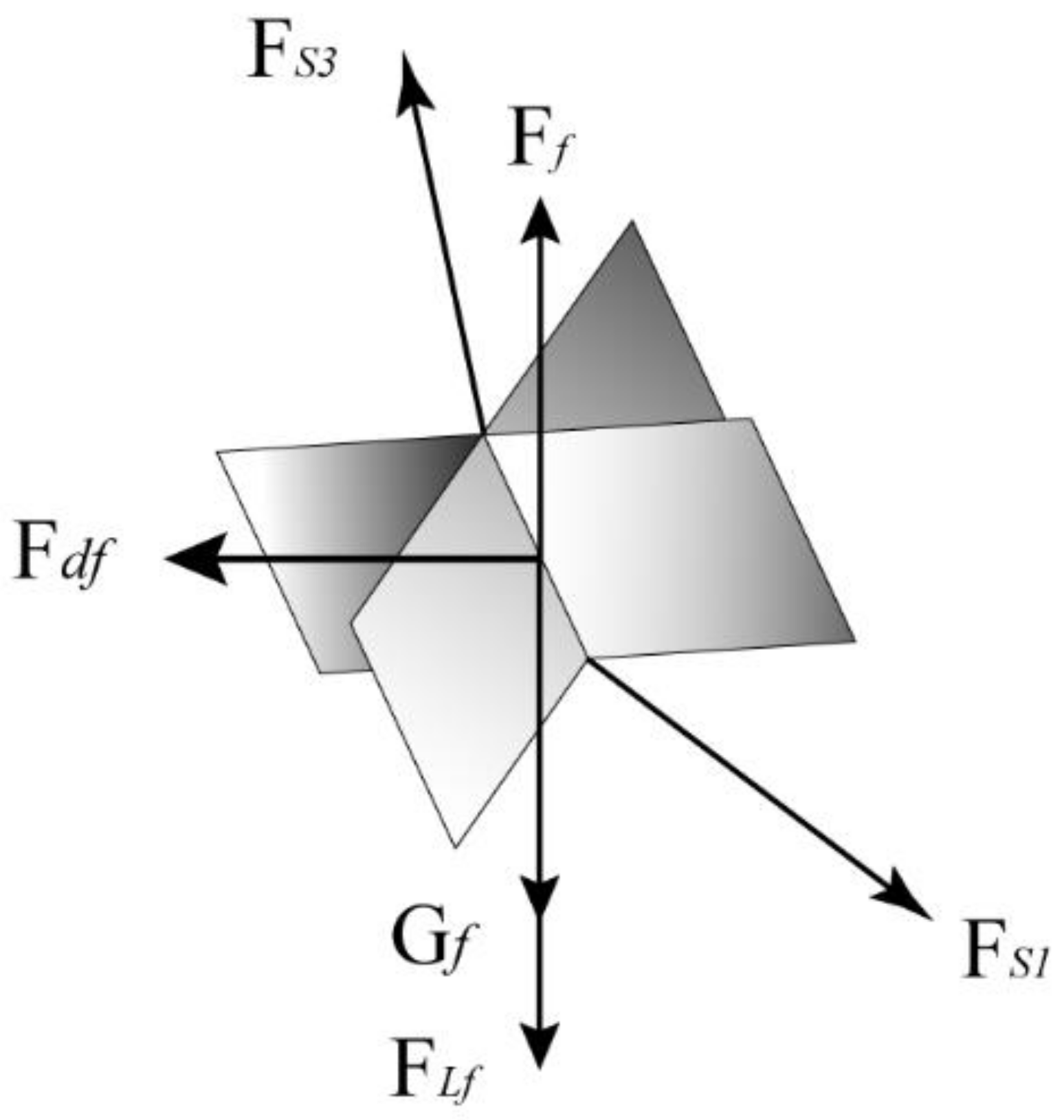
Figure 4 shows the force analysis of the cross-plate, where $F_f$ and $G_f$ are the cross-plate’s buoyancy and gravity, $F_{df}$ and $F_{lf}$ are the drag and lift of the flow around the cross-plate, which can be calculated by numerical simulations in Section 2.3, respectively, and $F_{s1}$ is the rope’s pull on the cross-plate.

In the horizontal direction and vertical direction, the force balance formula of the cross-plate is shown in Equations (8) and (9).

$$F_{s3}\sin {\theta }_3+F_f=G_f+F_{lf}+F_{s1}\sin {\theta }_1$$

(8)

$$F_{s3}\cos {\theta }_3+F_{df}=F_{s1}\cos {\theta }_1$$

(9)

Around point O, the torque balance equation is shown in Equation (10).

$$-c{F}_{s3}\sin \left({\theta }_3-{\theta }_2\right)+\frac{c}{2}\left( F_{lf}+G_f-F_f\right)\cos {\theta }_2+\frac{c}{2}{F}_{df}\sin {\theta }_2=0$$

(10)

Substituting Equations (4) and (5) into Equation (10), it can be found that

$$F_{lf}+F_{df}\tan {\theta }_2+2F_{dq}\tan {\theta }_2=2F_q-2G_q+F_f-G_f$$

(11)

Substituting Equations (4) and (5) into Equations (8) and (9), ${\theta }_1$ can be expressed as Equation (12). The vertical distance $H_t$ in theory can be expressed as Equation (13)

$${\theta }_1=\arctan \left(\frac{F_q-G_q+F_f-G_f-F_{lf}}{F_{dq}+F_{df}}\right)$$

(12)

$$H_t=L_{oc}\sin {\theta }_1$$

(13)

It can be seen from Equation (12) that to calculate ${\theta }_1$ and $H_t$, $F_{df}$ and $F_{lf}$ must be calculated first. This study calculates these two values through numerical simulations.

2.3. Numerical Simulations

In the numerical simulations, the acquisition of the $F_{df}$ and $F_{lf}$ values need to know the posture of the cross-plate in the flow field in advance (such as the incident angle). However, since the theory of Section 2.2 cannot directly calculate the value of ${\theta }_2$, in this section, it is necessary to simulate the flow field state of the cross-plate under the different incident angles when the velocity is the same. 30 cases of the flow around the cross-plate are simulated in three dimensions.

2.3.1. Pre-Processing

The pre-processing includes the definition of geometry and boundary conditions, grid generation, and solver parameters establishment.

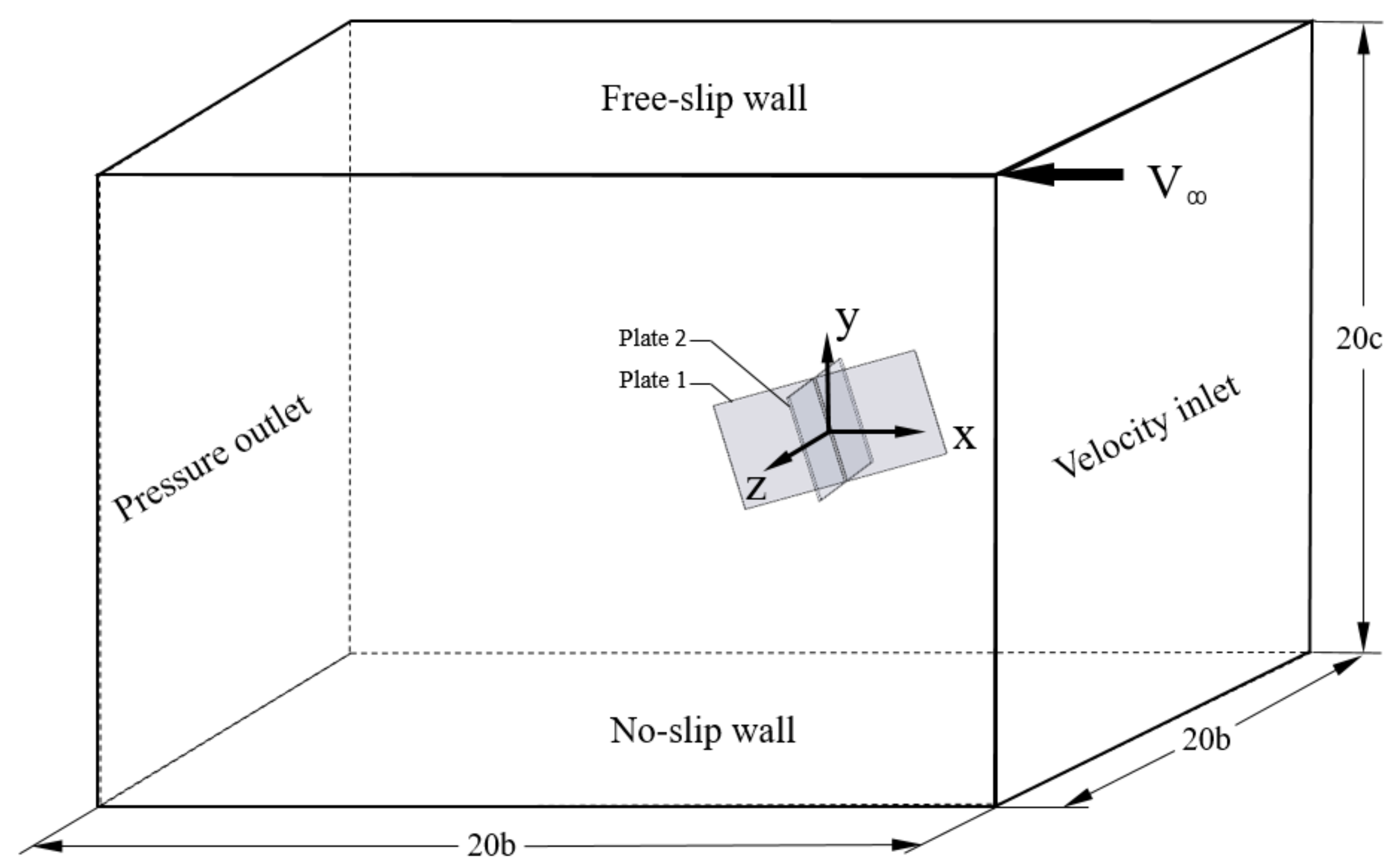
As shown in Figure 5, a Cartesian coordinate system was adopted such that the x-, y-, and z-axes are oriented in the streamwise, transverse, and spanwise directions, respectively. The origin of the coordinates was at the center of the axis of the cross-plate. Under the effect of the current, the central axis of the cross-plate may have a certain angle with the three coordinate axes. In the case of static simulation, it is difficult to simulate all the attitudes of the cross-plate. In most cases, there is a plate parallel to the direction of tidal velocity, which acts as a guide, such as “Plate1” in Figure 5. So the surrounding flow field of the cross-plate in this kind of posture (the center axis of the cross-plate is on the x-y plane) is simulated below.

The domain size is chosen such that the boundary conditions do not affect the flow field in the vicinity of the cross-plate. The computational domain for the present study was kept 20b in the x-direction, 20c in the y-direction and 20b in the z-direction. In the x-direction, the center of the cross-plate is located at 6.25b from the inlet for the full development of the flow without the influence of boundary effects. In the y-direction, the center of the cross-plate is symmetrical about the upper and lower boundaries. Similarly, in the z-direction, the center of the cross-plate is symmetrical about the front and rear boundaries. $V_{\infty }$ represents the current velocity in the x-direction.

A velocity inlet boundary condition with a constant velocity normal to the boundary was set on the right side corresponding to a pressure outlet on the left side. Except for the free-slip wall on the upper side, the other walls including the surface on the cross-plate are no-slip walls. Standard boundary wall condition is used at the base of the computational domain and on cross-plate surfaces and the values of Y+ were kept within the range of 0.5~7.

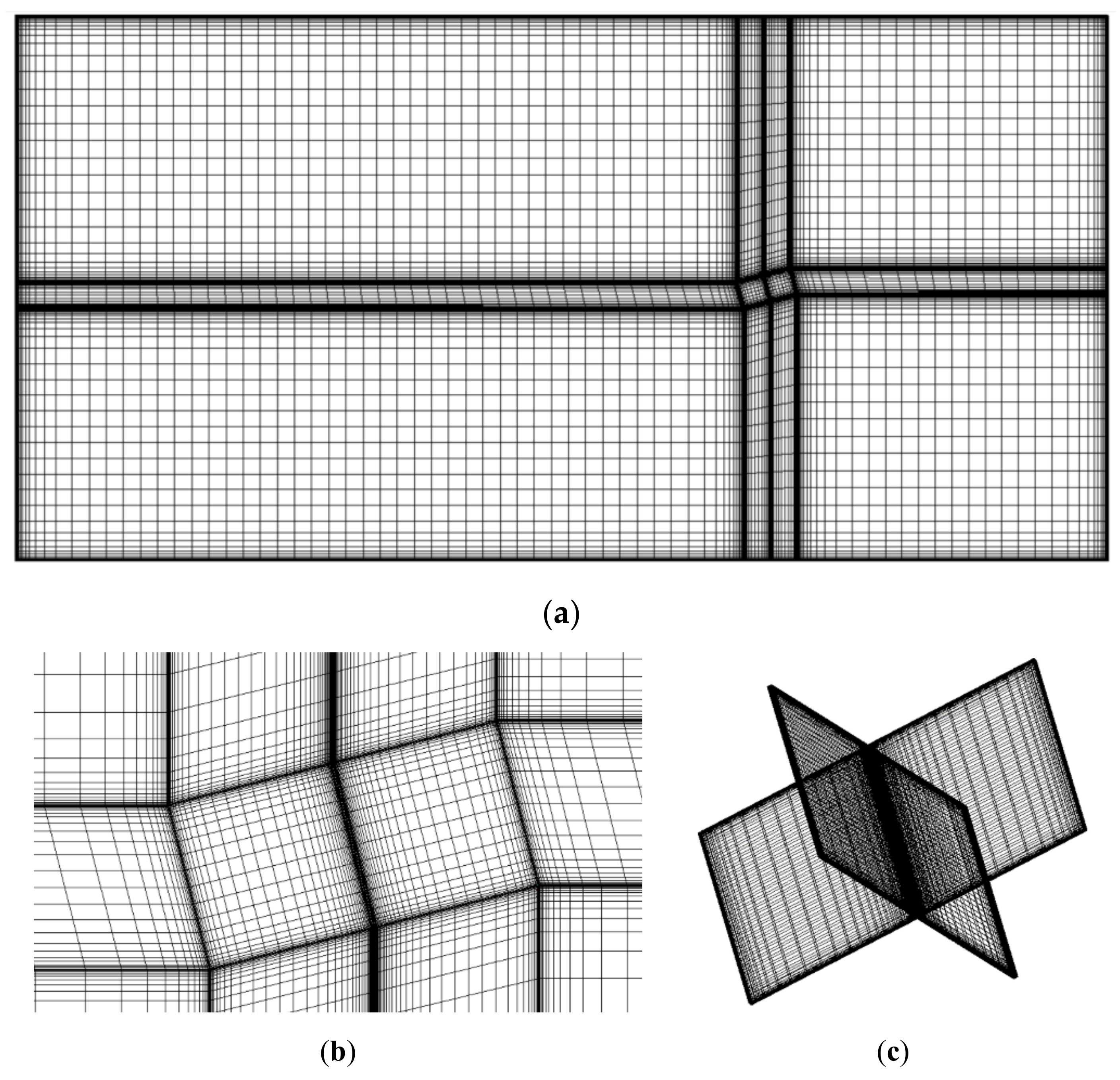
A total of 30 cases of cross-plates based on different flow incident angles $\mathsf{\alpha }$ and $V_{\infty }$, have been modeled and meshed using software ICEM CFD 19.0 in the present study. The simulation conditions have been listed in

Table 2. The characteristics of the cross-plate in the simulation cases: b = 16 cm, c = 8 cm, t = 0.2 cm, ρ = 998.2 kg/m³.

${\mathit{V}}_{\mathbf{\infty }} (\mathbf{m}/\mathbf{s})$	$\mathit{\alpha } (˚)$
	45	55	65	75	85	87
0.08	Case 1-1	Case 1-2	Case 1-3	Case 1-4	Case 1-5	Case 1-6
0.10	Case 2-1	Case 2-2	Case 2-3	Case 2-4	Case 2-5	Case 2-6
0.14	Case 3-1	Case 3-2	Case 3-3	Case 3-4	Case 3-5	Case 3-6
0.16	Case 4-1	Case 4-2	Case 4-3	Case 4-4	Case 4-5	Case 4-6
0.18	Case 5-1	Case 5-2	Case 5-3	Case 5-4	Case 5-5	Case 5-6

. The size of the cross-plate and current velocities set in the simulation are consistent with the corresponding parameters in the experiments. The computational domain was divided into 70 hexahedral blocks to generate structured meshes for better quality. As shown in Figure 6, the grids near the cross-plate region and wall condition boundaries were all refined with proper grid height. The 3D mesh model contains approximately 1.9 million to 3 million cells.

2.3.2. Governing Equations

The fluid in this simulation study meets the following four assumptions:

(a)

The fluid is Newtonian fluid;

(b)

The fluid is viscous and incompressible;

(c)

The fluid is three-dimensional;

(d)

The flow in the field is steady, and the flow parameters of the fluid clusters do not change with time.

The Navier-Stokes equation is the basic equation of fluid motion and is suitable for the turbulent model of flow around a cross-plate. The Navier-Stokes equation of an incompressible Newtonian fluid with constant viscosity can be written as follows.

Momentum equation:

$$\rho \frac{D{u}_i}{Dt}=\rho f_i-\frac{\partial p}{\partial x_i}+\mu \frac{{\partial }^2{u}_i}{\partial x_j^2}$$

(14)

where the velocity field $u_i$ satisfies the continuity equations

$$\frac{\partial u_i}{\partial x_i}=0$$

(15)

In Equations (14) and (15), $u_i$ are flow velocities in the three spatial directions, i.e., $i$ = 1 and 2 for the horizontal directions and i = 3 for the vertical direction, $D{u}_i/Dt$ is the material derivatives of $u_i$, $\rho$ is the fluid density, p is the pressure fluctuation, $f_i$ are the ith-component of body forces, $\mu$ is the kinematic viscosity of the fluid, t is time, and $x_i$ are the spatial coordinates.

Reynolds number of flow around the cross-plate in this study is in the range of $8.517\times {10}^3$~$1.965\times {10}^4$, so our research focuses on turbulent flow. In this study, it is not necessary to resolve the fine details of turbulent fluctuations, because the effects of each eddy are not of primary interest. By narrowing our focus and concentrating only on the mean turbulence variables, we can significantly reduce the number of calculation nodes to a manageable level and capture the pertinent features of the flow. For this reason, the RANS-based method was chosen for our research, which demands lesser computing resources and is available in FLUENT software and validated by a large number of experiments.

The selection of turbulence model depends on the specific problem, no turbulence model is suited for every case. Fine-tuning is required. To study the differences between these models in this research case in-depth, the standard 𝑘 − 𝜀 model, the standard k-ω model, and the shear stress transport (SST) model are used to simulate the flow field around the cross-plate at five different current velocities when the α is 75 degree. In the end, the results of the trial showed that the difference between the calculation results of these three models was not big, within 10%, so the standard 𝑘 − 𝜀 model was finally selected as the simulated turbulence model in this study. Two partial differential equations (transport equations) are solved in this type of turbulence model: the turbulent kinetic energy k and the turbulence eddy dissipation ε (i.e., the rate at which the turbulent kinetic energy dissipates) [29]. In this model, the following Equations (16) and (17) are used to obtain the turbulent kinetic energy and its rate of dissipation [30]:

$$\frac{\partial k}{\partial t}+\frac{\partial k{u}_i}{\partial x_i}=\frac{\partial }{\partial x_i}\left[\left(\nu +\frac{{\nu }_t}{{\sigma }_k}\right)\frac{\partial k}{\partial x_i}\right]+G_k+G_b-\epsilon$$

(16)

$$\frac{\partial \epsilon }{\partial t}+{\mathrm{U}}_{\mathrm{j}}\frac{\partial \epsilon }{\partial x_j}=\frac{\partial }{\partial x_j}\left[\left(\nu +\frac{{\nu }_t}{{\sigma }_{\epsilon }}\right)\frac{\partial \epsilon }{\partial x_j}\right]+C_{\epsilon 1}\frac{\epsilon }{k}\left(G_k+C_{\epsilon 3}{G}_b\right)-C_{\epsilon 2}\frac{{\epsilon }^2}{k}$$

(17)

where ${\sigma }_{\epsilon }$ is the turbulent Prandtl number for $\epsilon$ and is assumed as equal to 1.3, ${\sigma }_k$ is the turbulent Prandtl number for $k$ and is assumed as equal to 1.

The equation for the turbulent kinematic viscosity at each point is:

$$v_t=C_u\frac{k^2}{\epsilon }$$

(18)

$G_k$ is the generation of turbulent kinetic energy due to mean velocity gradients, which is common in most turbulence models, and is given by:

$$G_k=2{\nu }_t{S}_{ij}{}^2$$

(19)

where the strain-rate tensor is $S_{ij}$ written as:

$$S_{ij}=0.5\left(\frac{\partial u_j}{\partial x_i}+\frac{\partial u_i}{\partial x_j}\right)$$

(20)

$G_b$ represents the generation of turbulent kinetic energy due to buoyancy, which can be expressed as:

$$G_b=-u_t\frac{g}{\rho }\frac{\partial \rho }{\partial y}$$

(21)

Furthermore, the constants $C_{\epsilon 1},$ $C_{\epsilon 2}$ and $C_u$ have the following default values in this study:

$$C_{\epsilon 1}=1.44, C_{\epsilon 2}=1.92, C_u=0.09$$

Version 19.0 of the Ansys-Fluent software was used based on a finite volume approach with a double-precision solver. A pressure-based solver was selected for all numerical simulations. In these cases, the water temperature is uniformly set to 20 °C in the whole computational domain. The coupled algorithm was used for the pressure-velocity coupling. For solving convection and viscous terms of the governing equation, all discretization items such as pressure, momentum, turbulent kinetic energy, and turbulent dissipation rate were set to second-order upwind discretization schemes. The turbulence conditions on velocity inlet and pressure outlet boundaries were specified by the turbulent intensity and hydraulic diameter. The turbulent intensity was set to 5%. The 1000 steps were iterated to obtain the time-averaged results for the steady analyses. An absolute convergence criterion of ${10}^{-6}$ was chosen for the convergence of velocity and continuity equations.

2.3.3. Grid Independence Analysis

The grid needs to be fine enough to resolve the boundary layer formed near the cross-plate surfaces, yet the computational cost will increase simultaneously as the grid size diminishes. To find a reasonable grid size, four meshes with different degrees of refinement were generated, which means that the meshes near the cross-plate were changed while the meshes away from the cross-plate were not changed. Their mesh numbers are shown in

Table 3. Parameters of four simulation cases for grid independence verification: c = 0.08 m, b = 0.16 m, t = 0.002 m, $V_{\infty }=0.12 \mathrm{m}/\mathrm{s}$, incident angle $\mathsf{\alpha }=11.9°$, $\mathsf{\rho }=998.2\frac{\mathrm{kg}}{m^3}, \mathrm{T}=20$ °C.

Case	$$\mathsf{∆}\mathbf{d} \left(\mathbf{mm}\right)$$	Mesh Number
1	0.8	887814
2	0.6	1873399
3	0.3	3809366
4	0.1	6518992

, where $\mathsf{∆}\mathrm{d}$ is the size of the smallest grid on the cross-plate.

The force problem of the cross-plate is closely related to the pressure distribution on the surface of the cross-plate, so Figure 7 shows the pressure distribution on the intersection of the y = 0 surface and the right side of the cross-plate.

Results of Figure 7 show that there is no significant discrepancy of the simulation results on the four grid resolution. To summarize, the grid independence results suggest that the four grid resolutions within a range can accurately capture the hydrodynamic boundary layers on the cross-plate in this study. The following simulation case uses $\mathsf{∆}\mathrm{d}$ = 0.3 mm as the minimum interval of the grid.

3. Experimental Setup and Methods

3.1. Facility and Setup

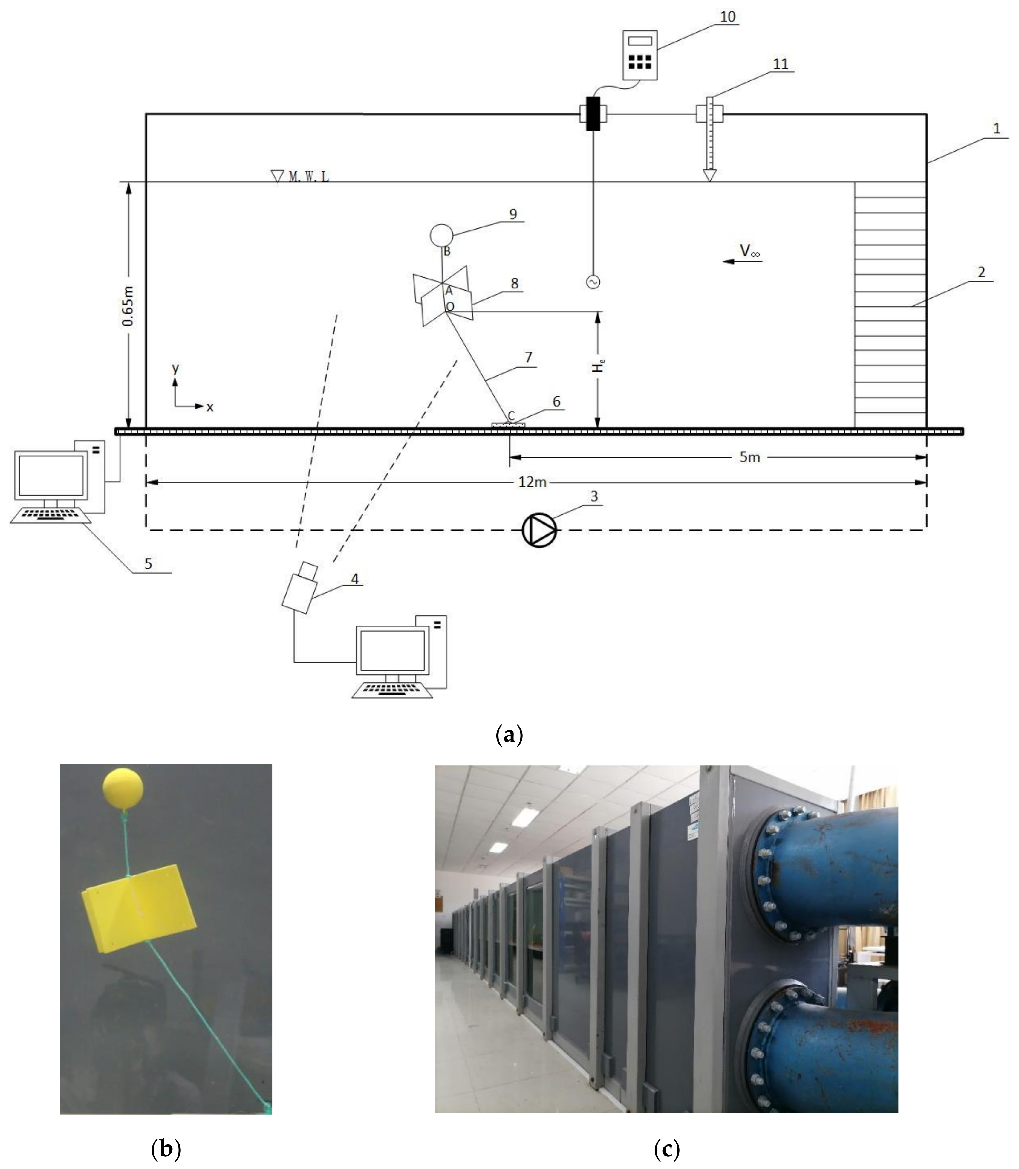
The experiments were conducted in the flume at the Hydraulics Laboratory of Zhejiang University (China) to verify the theoretical model as well as to experimentally study the effect of current velocity on the performance of the profiler. Figure 8 is a schematic diagram of the experimental setup. As shown in Figure 8, the experimental equipment is composed of a flume, a set of profiler equipment, various measuring facilities, and other auxiliary equipment. The nomenclatures (such as b, c, t,${\theta }_{1,}$ ${\theta }_2$, ${\theta }_3$,$L_{AB}$, $L_{OC}$, $V_{\infty }$ and $\rho , \mathrm{etc}.$) appearing in this part and the definition of the coordinate system are the same as the nomenclatures and coordinate system definition of the theory part, and will not be repeated here.

The flume is 12 m long, 0.6 m wide with an available depth of 0.8 m. The flume is capable of generating constant currents for different velocities by changing the inlet current velocity and the opening degree of the outlet water valve. The flume is equipped with a flow pump driven by an electrical motor with a maximum flow rate of 1300 m³/h. The vibrant nature of the pump makes it necessary to install a set of honeycomb tubes whose height overtops the water level to dampen current fluctuation and smooth turbulence on the incoming flow. The experimental apparatus was installed 5 m from the flume entrance. A high-resolution acoustic velocimeter named Vectrino was used to measure the current velocities in the flume. The basis measurement technology of Vectrino is coherent Doppler processing, which is characterized by accurate data with no appreciable zero offset. The sampling rate was set to 5 Hz, which was enough to satisfy the accuracy requirement. A high-definition camera (SONY, HDR-PJ675) with a sampling rate of 25 fps was mounted on one side of the flume to record a video sequence of the rope tilt angle.

3.2. Similarity Design and Test Conditions

For the model test to be able to show the prototype phenomenon from the physical essence, it is necessary to use similar principles to determine the geometric and hydrodynamic parameters of the experimental model. Since the Newton number $N_e$ can describe the influence of the resistance generated by the moving fluid, it is taken as the main similarity criterion number in this study. $N_e$ can be expressed as Equation (22).

$$N_e=f\left(R_e,r\right)$$

(22)

Among them, $R_e$ is the Reynolds number and $r$ is the geometric ratio of the object in the fluid. Therefore, to ensure the flow similarity between the model and the prototype, the following two similarity conditions must be met.

$$R_{em}=\frac{{\rho }_m{V}_m{b}_m}{{\mu }_m}=\frac{{\rho }_p{V}_p{b}_p}{{\mu }_p}=R_{ep}$$

(23)

$$r_m=\frac{b_m}{c_m}=\frac{b_p}{c_p}=r_p$$

(24)

In Equation (23), $\mu$ is fluid viscosity, subscript m represents the model used in the tank experiment, p represents the prototype of the sea area, and the meaning of the remaining symbols is the same as in Section 2. Therefore, the partial parameters of the flume experiments can be designed, as shown in

Table 4. Part of the experimental parameters of the flume obtained according to similar criteria.

	Model	Prototype
Dynamic viscoity μ (N·s/m2)	1.14 × 10−3	1.20 × 10−3
Fluid density ρ (kg/m3)	998.2	1018.25
The size of cross-plate (cm)	b = 16, c = 8	b = 5.50, c = 2.75
Current velocities $V$ (m/s)	0.08, 0.10, 0.14, 0.16, 0.18	0.24, 0.30, 0.42, 0.48, 0.54

.

Since the focus of this study is to discuss the influence of current velocities on the vertical position of the profiler, geometric parameters such as the size of the cross-plate and the size of the float are kept constant. The set of profiler equipment includes a buoy with a diameter of 5 cm, a cross-plate, a weight of 1.34 kg, and a nylon cable connecting various components. The buoy is an empty spherical shell with a wall thickness of 2 mm obtained by 3D printing. The buoy mass is 20.9 g, which can produce a buoyancy of 0.64 N when completely immersed in the liquid. The highest position of the buoy was 0.15 m below the water surface, which is enough to eliminate the influence of the boundary effect. The cross-plate is composed of two identical plastic thin plates of height 8 cm, width 16 cm, and thickness 0.2 cm ensuring no deformations took place during the experiments. The mass of the cross-plate is 61.65 g. The length of the rope AB and OC are 0.07 m and 0.3 m, respectively. At the beginning of the experiment, the central axis of the cross-plate was equidistant from the front and rear walls of the flume.

In the experiments, the water level of the experiments was maintained at 0.65 m with ±0.2 cm error and is recorded by a water level gauge fixed on the flume. A total of 5 experiments were carried out at current velocities of 0.08, 0.10, 0.14, 0.16, and 0.18 m/s.

3.3. Experimental Procedure

Primarily, the preparations for the experiments need to be done. The velocimeter was calibrated and configured correctly, and fixed at the platform, which was on the slide rails installed at both top edges of the flume. When measuring current velocities, the probe of the velocimeter is in the same depth. During the experiment, the probe of the velocimeter is located more than 0.5 m upstream of the test device to minimize the impact on the flow field near the profiler model.

The experiments were divided into five groups according to five different current velocities. The operation procedure of the experiments is as follows:

(1)

Startup the pumping system, and then adjust the flow rate and opening degree of the outlet water valve of the flume by upper computer software, until the display of the water level gauge is 0.65 m.

(2)

Connect the buoy, cross-plate, and weight with ropes, and adjust the spacing between them as shown in Figure 8.

(3)

Place the experimental equipment 5 m from the entrance of the flume. Adjust the position of the cross-plate to the symmetry of the front and rear walls. Observe the posture of the rope in the fluid to see if the rope is tight when the fluid is at rest.

(4)

Adjust the x-axis velocity of the velocimeter is in the range of $V_{\infty }$ ± 0.005 m/s. $V_{\infty }$ is one of the five different current velocities enumerated previously.

(5)

Record the water temperature and open the camera to record the whole process of the group of tests.

(6)

Repeat step (1) to (5), until all current velocities are tested. For each combination, a repetition of three times is at least.

4. Results and Discussion

4.1. Comparison of the Vertical Motion Range of the Profiler in Theory and Flume Experiments

In this study, the force of the cross-plate was calculated by numerical simulation to make up for the shortcomings of static force analysis, that is, numerical simulation is only an auxiliary tool, and the theoretical results obtained by the combination of the two are compared with the results of the flume experiment.

The vertical distance $H$ between point O and point C reflects the vertical movement range of the profiler. It can be seen from Equation (13) that to calculate the value of $H_t$, the values of ${\theta }_1$, $F_{df}$, $F_{lf}$ and ${\theta }_2$ must be calculated first.

For simulation cases with different incident angles and different current velocities, both $F_{df}$ and $F_{lf}$ can be calculated, as shown in

Table 5. Values of $F_{df}$, $F_{lf}$ and Y in different simulation cases.

Case	${\mathit{V}}_{\mathbf{\infty }} (\mathbf{m}/\mathbf{s})$	$\mathit{\alpha } (˚)$	${\mathit{F}}_{\mathit{d}\mathit{f}} \left(\mathbf{N}\right)$	${\mathit{F}}_{\mathit{l}\mathit{f} }\left(\mathbf{N}\right)$	$\mathit{Y}$ (N)
1-1	0.080	45	0.054	0.003	1.131
1-2		55	0.054	0.005	0.621
1-3		65	0.052	0.013	0.209
1-4		75	0.048	0.021	0.123
1-5		85	0.041	0.026	0.084
1-6		87	0.033	0.029	0.062
2-1	0.104	45	0.091	0.005	1.903
2-2		55	0.091	0.008	1.044
2-3		65	0.088	0.023	0.353
2-4		75	0.080	0.036	0.208
2-5		85	0.068	0.045	0.142
2-6		87	0.055	0.049	0.104
3-1	0.142	45	0.168	0.009	3.529
3-2		55	0.168	0.014	1.936
3-3		65	0.164	0.042	0.655
3-4		75	0.149	0.067	0.386
3-5		85	0.126	0.083	0.263
3-6		87	0.101	0.092	0.193
4-1	0.164	45	0.223	0.011	4.697
4-2		55	0.224	0.019	2.578
4-3		65	0.219	0.057	0.874
4-4		75	0.199	0.089	0.515
4-5		85	0.167	0.111	0.350
4-6		87	0.134	0.122	0.257
5-1	0.184	45	0.281	0.014	5.904
5-2		55	0.282	0.024	3.242
5-3		65	0.275	0.071	1.099
5-4		75	0.250	0.112	0.648
5-5		85	0.210	0.140	0.440
5-6		87	0.168	0.154	0.323

. Define that the left side of Equation (11) is equal to $Y$, as in Equation (25), and the value of Y is listed in the last column of Table 5. The directions of $F_{df}$ and $F_{lf}$ in Table 5 are opposite to the direction of the coordinate axis, and should be negative values. To facilitate reading, their absolute values are displayed in the table.

$$Y=F_{lf}+F_{df}\tan \alpha +2F_{dq}\tan \alpha$$

(25)

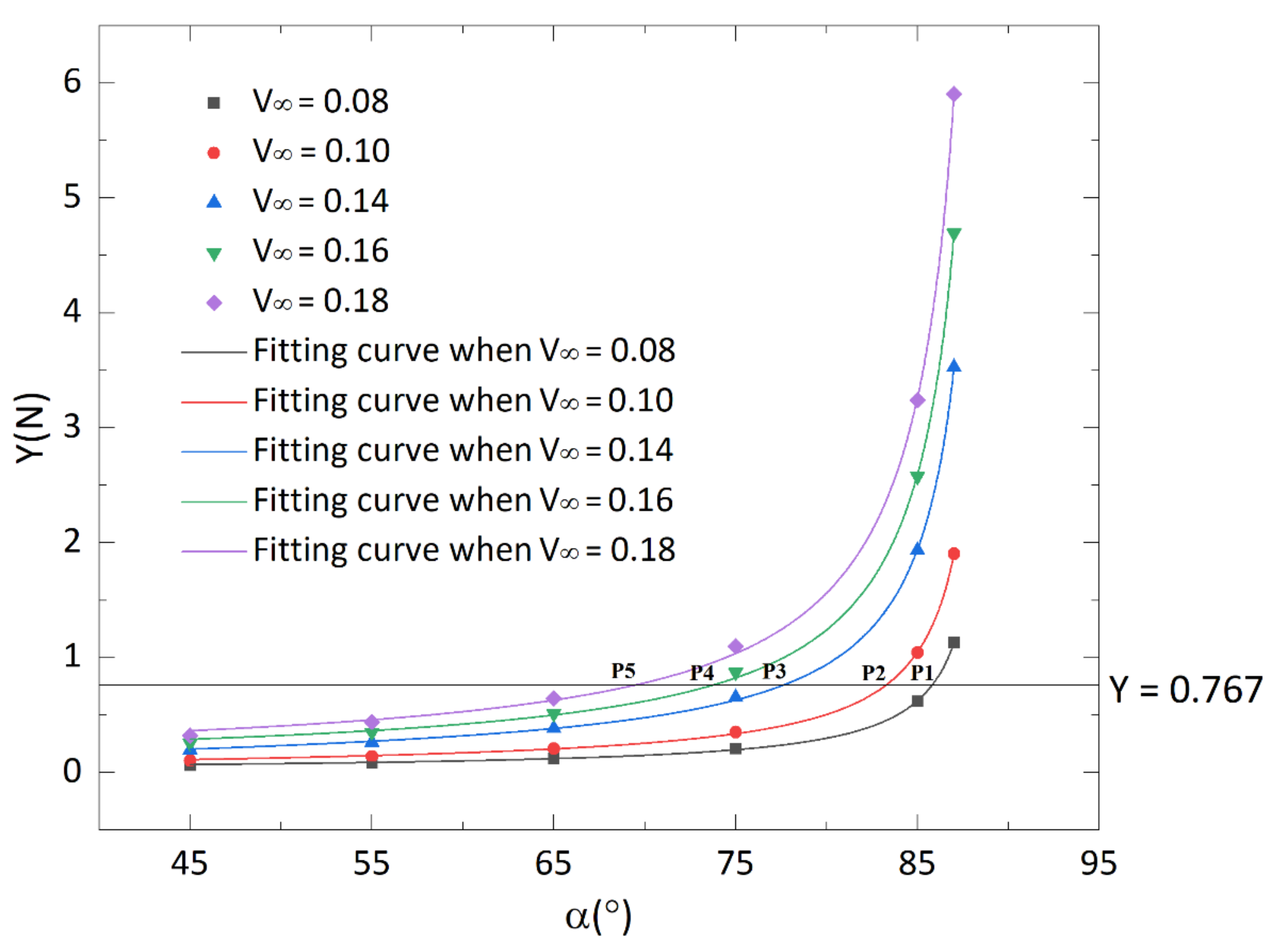
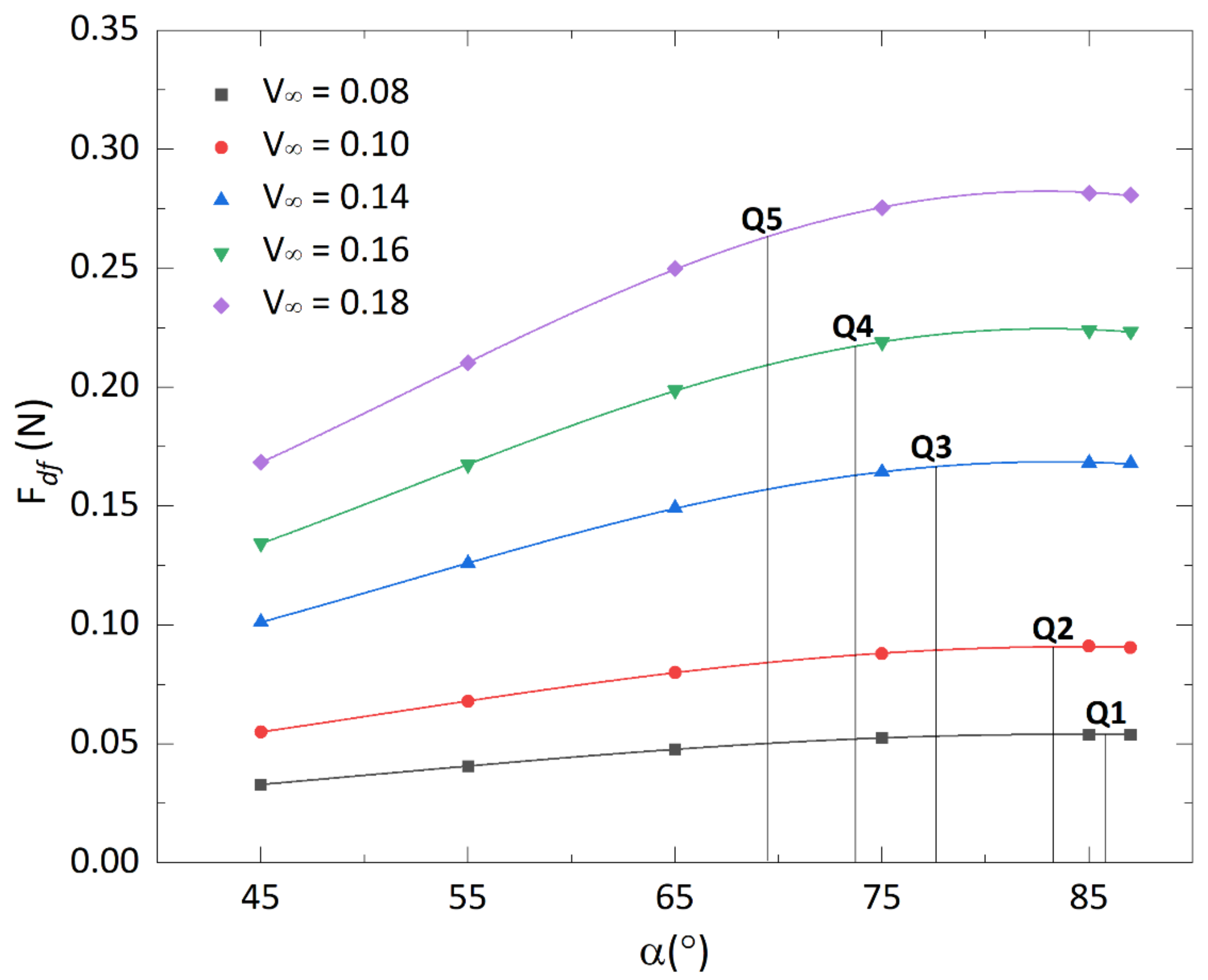
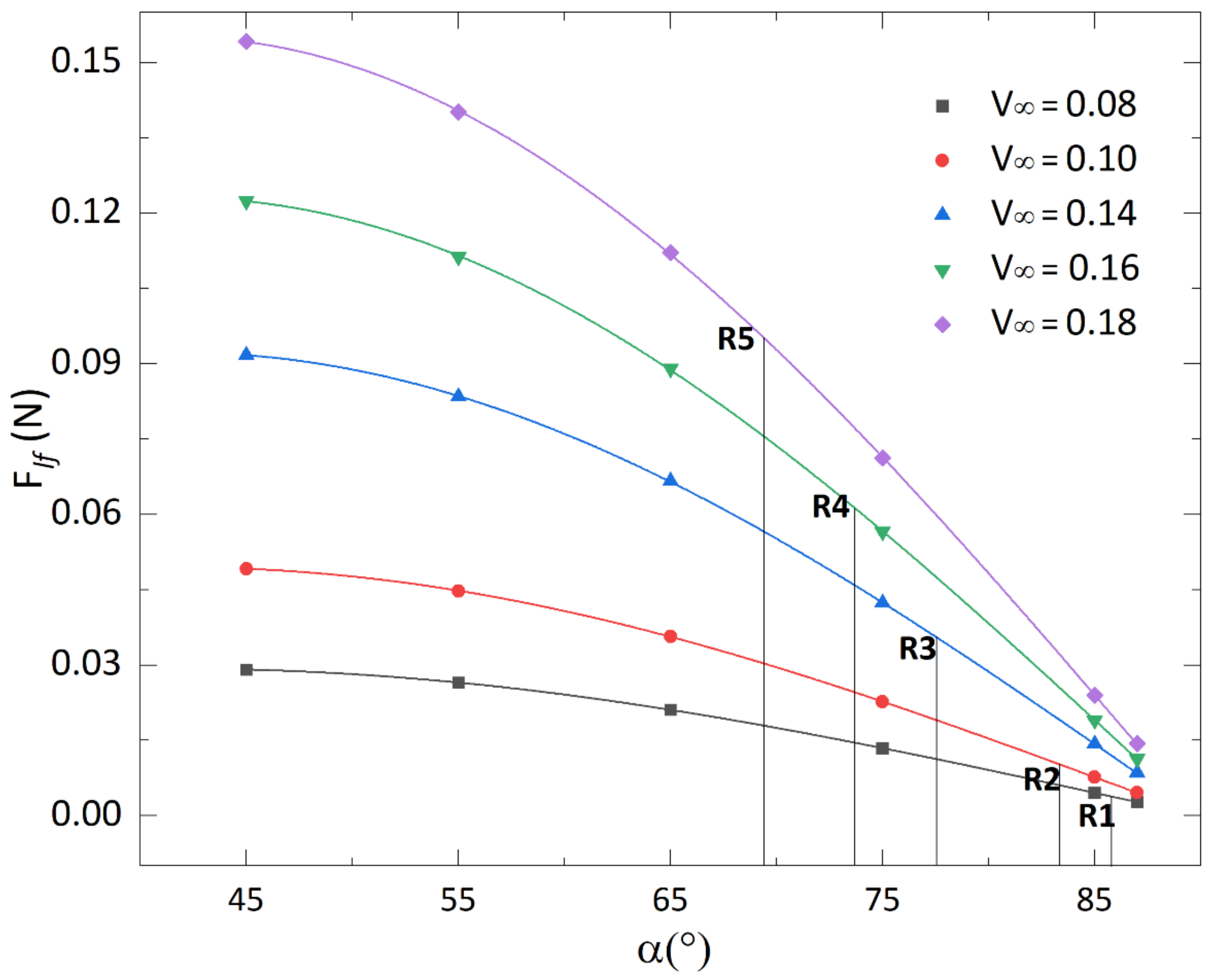
According to the data in Table 5, Figure 9, Figure 10, Figure 11 can be drawn, which respectively show the variation of $Y, F_{df}$ and $F_{lf}$ with the incident angle α under different current velocities. Use the function $a+b\tan \left(cx+d\right)$ to fit each set of data points in Figure 9 to obtain 5 fitting curves.

Since the right side of Equation (11) is a constant and equal to 0.767, draw the line Y = 0.767 in Figure 9. This line and the five fitting curves in the figure intersect at five points: points P1, P2, P3, P4, and P5, and the abscissa and ordinate of these 5 points are shown in

Table 6. The abscissa and ordinate from points P1 to P5, Q1 to Q5, and R1 to R5.

Points	Abscissa	Ordinate	Points	Abscissa	Ordinate	Points	Abscissa	Ordinate
P1	85.802	0.767	Q1	85.802	0.054	R1	85.802	0.004
P2	83.283	0.767	Q2	83.283	0.091	R2	83.283	0.010
P3	77.619	0.767	Q3	77.619	0.167	R3	77.619	0.035
P4	73.734	0.767	Q4	73.734	0.217	R4	73.734	0.061
P5	69.474	0.767	Q5	69.474	0.263	R5	69.474	0.095

.

The abscissa of P1 to P5 is the theoretical value of ${\theta }_2$ under the corresponding current velocity. For example, the coordinate of point P1 is (85.802, 0.767), and 85.802° is the theoretical value of ${\theta }_2$ when the current velocities is 0.08 m/s. Use the function $a+b\sin \left(cx+d\right)$ to fit each group of data points in Figure 10 to obtain 5 fitting curves. Draw the vertical line $\alpha =85.802$ and intersect the fitting curve corresponding to the velocity of 0.08 m/s at point Q1. The ordinate of Q1 is the drag force $F_{df}$ of the cross-plate when the current velocity is equal to 0.08 m/s. Use the same method to find the positions of points Q2 to Q5.

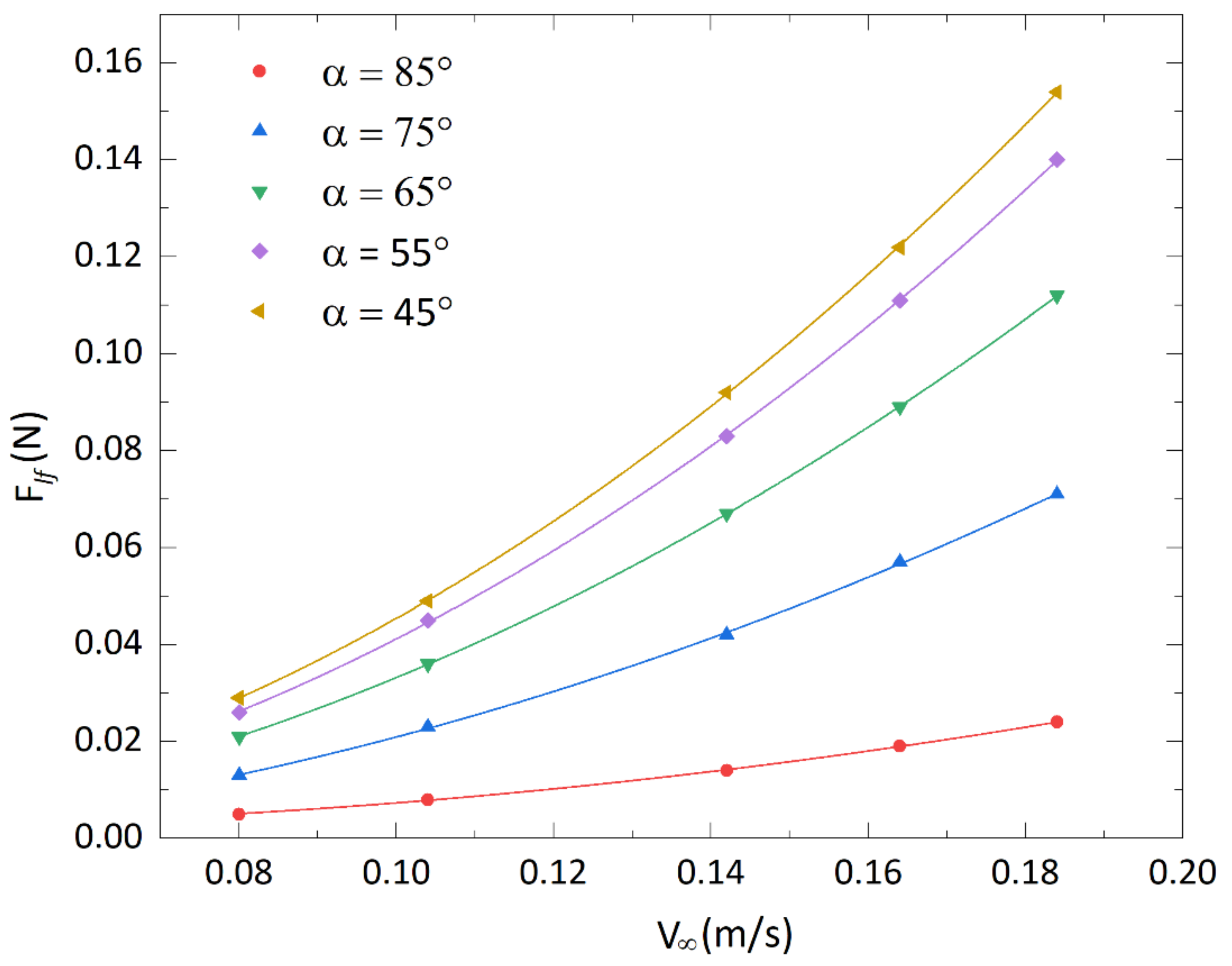
Use the function $a+b\cos \left(cx+d\right)$ to fit each group of data points in Figure 11 to obtain 5 fitting curves. Draw the vertical line $\alpha =85.802$ and intersect the fitting curve corresponding to the velocity of 0.08 m/s at point R1. The ordinate of R1 is the lift force $F_{lf}$ of the cross-plate when the current velocity is equal to 0.08 m/s. Use the same method to find the positions of points R2 to R5.

Substituting $F_{df}$ and $F_{lf}$ into Equation (12), ${\theta }_1$ can be calculated at a certain current velocity. Substituting ${\theta }_1$ into Equation (13), the vertical height $H_t$ from point O on the cross-plate to point C at the end of the rope can also be calculated.

In the experiment, even at the same current velocity, the value of ${\theta }_1$ is not fixed, but fluctuates within a certain range. Therefore, it is necessary to measure the minimum and maximum values of ${\theta }_1$ in the experimental video at a certain current velocity, and then calculate the minimum and maximum values of the vertical distance $H_e$ between point O and point C. The values of $H_t$ and $H_e$ are listed in

Table 7. The values of $H_t$ and $H_e$ at different current velocity.

${\mathit{V}}_{\mathbf{\infty }}$ (m/s)	${\mathit{H}}_{\mathit{t}}$ (cm)	${\mathit{H}}_{\mathit{e}-\mathit{m}\mathit{i}\mathit{n}}$ (cm)	${\mathit{H}}_{\mathit{e}-\mathit{m}\mathit{a}\mathit{x}}$ (cm)	${\mathit{H}}_{\mathit{e}-\mathit{a}\mathit{v}\mathit{g}}$ (cm)
0.08	29.559	29.336	29.850	29.593
0.10	28.752	26.274	28.657	27.465
0.14	25.803	15.644	25.166	20.405
0.16	22.883	10.295	24.466	17.381
0.18	19.428	1.309	21.328	11.318

. In this table, $H_{e-min}$, $H_{e-max}$ and $H_{e-avg}$ respectively represent the minimum, maximum and average value of $H_e$ at a certain current velocity.

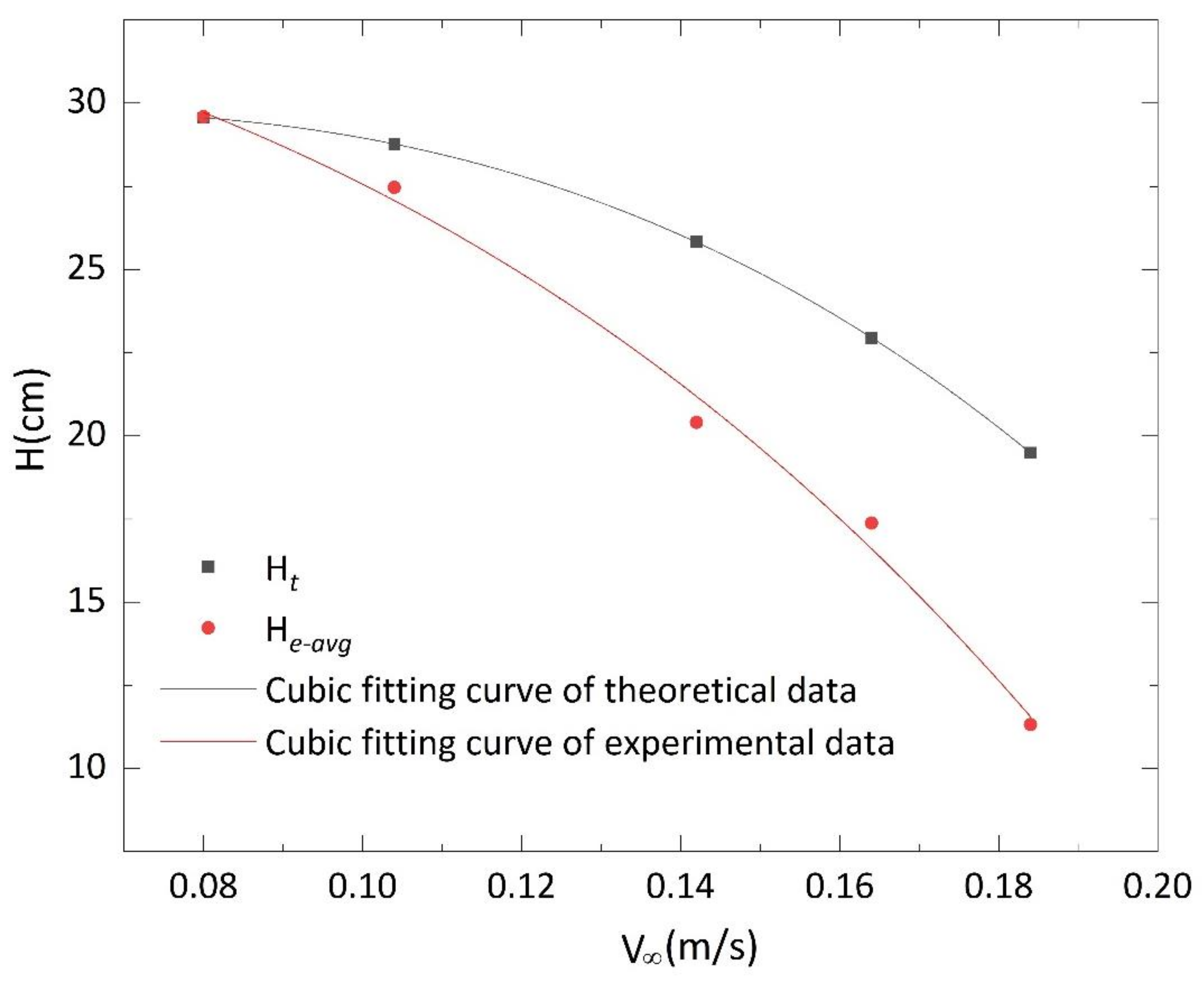
From the data in Table 7, it can be found that the range of $H_e$ varies from 1.309 cm to 29.850 cm. Since the length of the rope OC is only 30 cm, the cross-plate realizes the vertical ascending and descending movement within the maximum range. $H_t$ is basically between $H_{e-min}$ and $H_{e-max}$.

According to the data in Table 7, Figure 12 can be drawn, which shows that at the same current velocity, although the theoretical value of $H_t$ is not less than the experimental average, the theoretical change trend of the vertical height $H$ is similar to the experimental change trend. As the current velocity gradually increases, the vertical height $\mathrm{H}$ will gradually decrease.

4.2. The Effect of Current Velocity on System Motion Stability

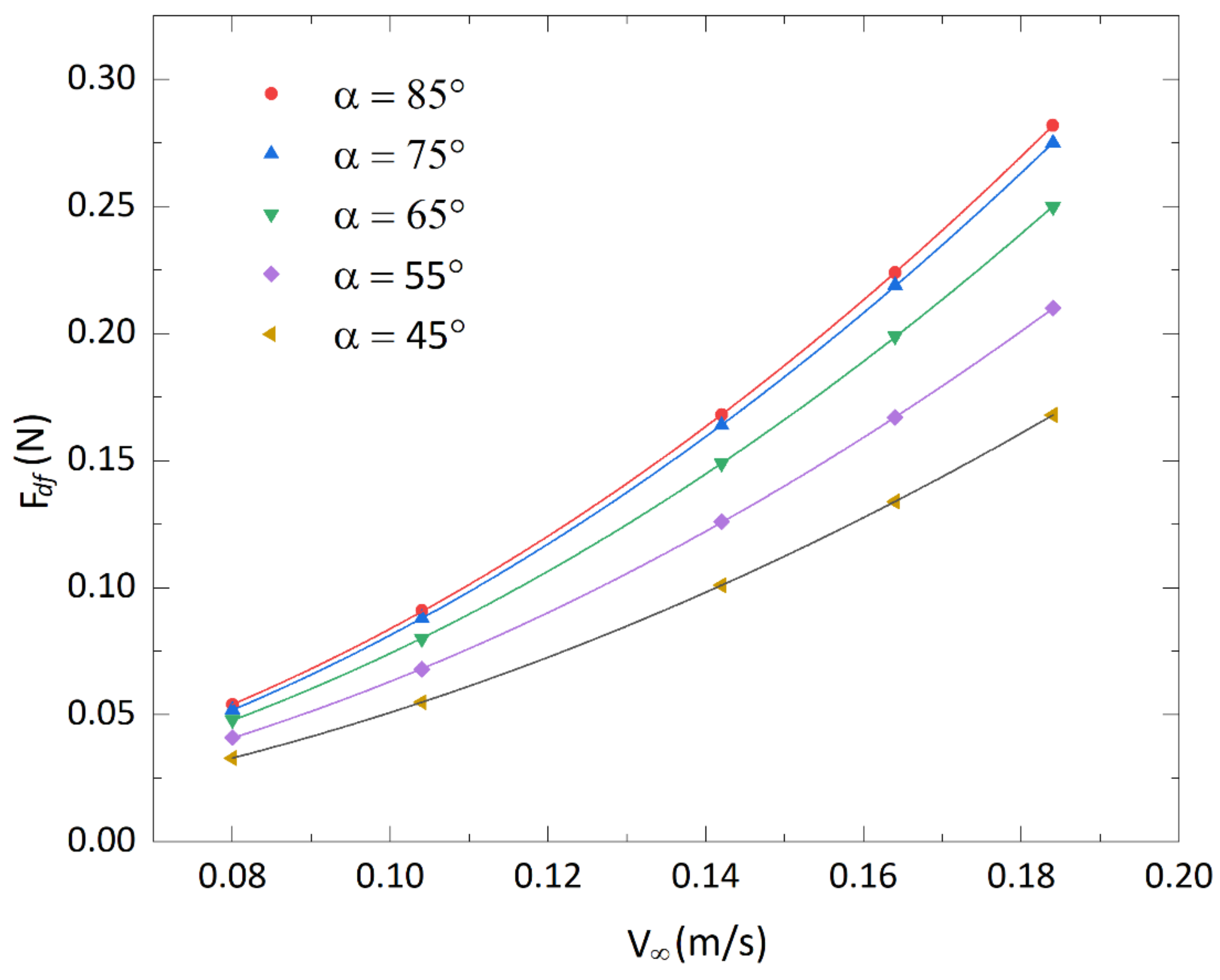
It was observed during the experiment that when the preset current velocity is fixed, the cross-plate sometimes swings clockwise around point C and sometimes counter-clockwise. Besides, from the data in Table 7, it was found that as the current velocity increases, the range of the distance between the cross-plate and the bottom of the flume will increase, that is, the subtraction of $H_{e-max}$ and $H_{e-min}$ will increase. The instability of the cross-plate movement has increased and the gap between theory and experiment will become relatively obvious just as shown in Figure 12. This may be due to the sensitivity of the cross-plate to changes in current velocity and the instability of the actual current velocity. The former is reflected in the fact that although the range of current velocity in the experiment is only 0.1 m/s, the height change of the cross-plate reaches 28.541 cm. This distance is almost equal to the rope length $L_{oc}$, which also means that the cross-plate realizes the movement from position I to position IV shown in Figure 1. The latter is reflected in the fact that although a honeycomb tube is installed in the flume, it does not guarantee that the current is absolutely uniform. With the increase of the current velocity, this unevenness will become more obvious. The geometric position of the cross-plate reciprocates within a certain range, which must be caused by the breaking of the original force balance relationship of the cross-plate, that is, its force in the flow field has changed. Therefore, the influence of the current velocity on the force $F_{df}$ and $F_{lf}$ of the cross-plate is analyzed respectively, as shown in Figure 13 and Figure 14.

Assuming that the cross-plate was originally at position II, as shown in Figure 1, due to unstable speed, when the current velocity increases, it is found from Figure 13 and Figure 14 that $F_{lf}$ and $F_{lf}$ will increase accordingly, so the cross-plate will deviate from the original position and move down to position III. If the speed decreases at this time, $F_{df}$ and $F_{lf}$ will decrease accordingly, and the cross-plate will move up from position III to position II. Moreover, the greater the speed, the greater the Reynolds number, which intensifies the instability of the flow, and makes the cross-plate reciprocating more violently, which ultimately makes the gap between theory and experiment more obvious.

4.3. The Influence of the Velocity in the Z-Direction on the Experimental Results

Figure 12 is drawn on the assumption that there is only a current velocity in the y-direction. However, in the actual experiment, due to the instability of the turbulent flow, the velocity in the z-direction is not zero. So it is necessary to discuss the influence of the velocity in the z-direction on the experimental height $H_e$.

As shown in Figure 15, by shooting the motion posture of the profiler directly above, the deflection angle $\theta$ was measured between the rope OC and the horizontal line, and the statistical results recorded in

Table 8. Horizontal offset angles of the cross-plate in flume experiments.

${\mathit{V}}_{\mathbf{\infty }}$(m/s)	${\mathit{\theta }}_{-} \left(°\right)$	${\mathit{\theta }}_{+} \left(°\right)$	$\mathit{\theta }$
0.080	−2.50	3.00	3.00
0.104	−4.00	3.29	4.00
0.142	−8.50	7.68	8.50
0.164	−9.88	10.42	10.42
0.184	−10.98	11.50	11.50

.

In Table 8, ${\theta }_{+}$ is the deflection angle along the counterclockwise direction, and ${\theta }_{-}$ is the deflection angle along the clockwise direction, and $\theta$ is the maximum value of the absolute value of ${\theta }_{+}$ and ${\theta }_{-}$.

Correct the experimental curve in Figure 12 according to the value of $\theta$, and one draws Figure 16.

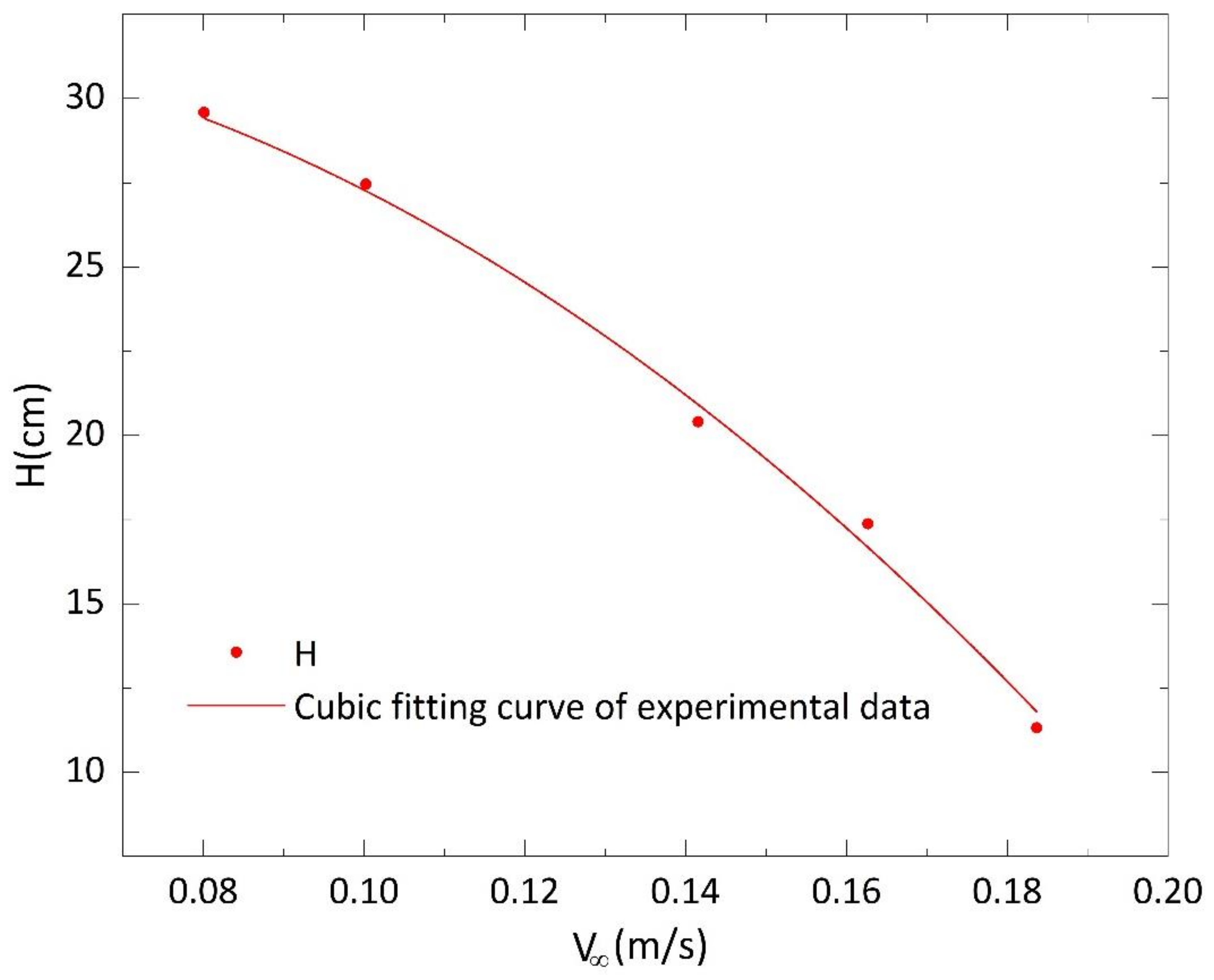
According to Figure 12 and Figure 16, the height H under the corresponding current velocity can be obtained, and their percentage error can be calculated, as shown in

Table 9. Comparison of height H when considering whether the flow velocity in the z-direction or not.

${\mathit{V}}_{\mathbf{\infty }} (\mathbf{m}/\mathbf{s})$	${\mathit{H}}_{\mathit{o}} \left(\mathbf{cm}\right)$	${\mathit{H}}_{\mathit{n}} \left(\mathbf{cm}\right)$	Deviation (%)
0.08	29.58	29.57	0.02
0.1	27.43	27.41	0.09
0.14	21.24	20.95	1.43
0.16	17.20	16.63	3.28
0.18	12.55	11.62	8.31

.

The $H_o$ in Table 9 comes from the experimental fitting curve in Figure 14, and $H_n$ comes from Figure 16. The percentage error of the two is listed in the last column.

It can be found that the deviation value is less than 10%, so the influence of the current velocity in the z-direction on the height H can be ignored.

5. Conclusions

This study shows that the tidal currents can drive the ups and downs of the observation platform on the profiler when driving the cross-plate to rise and fall, to achieve continuous recording and measurement of ocean profile parameters. Through dynamic analysis, combined with numerical simulations, a theoretical model of the system’s posture in the water is established. Although it cannot accurately calculate the position of the observation platform in the system under a certain current velocity, the comparison results with the flume experiments can prove that the model can roughly predict the movement trend of the entire system. Furthermore, the results of the deployment prove that tidal energy can be used as a kind of energy to drive the profiler’s ascent and descent motion and to measure ocean parameters without using electric energy. Moreover, the influence of current velocity changes on the stability of the entire system is analyzed, which is one of the contents that need to be studied in depth in the future. This profiler can be deployed on a large scale in the coastal waters with currents and has the advantages of low cost, good reliability, and easy maintenance. Next, we can explore the influence of the size of the cross-plate on the profiler’s range of activity and add a buoyancy adjustment mechanism as an auxiliary means to actively control the vertical movement of the horizontal plate in the water.

References

- Jouffroy, J.; Zhou, Q.; Zielinski, O. Towards Selective Tidal-Stream Transport for Lagrangian profilers. In Proceedings of the Oceans’11 MTS/IEEE KONA, Kona, HI, USA, 19–22 September 2011. [Google Scholar]
- Dabholkar, N.; Desa, E.; Afzulpurkar, S.; Madhan, R.; Navelkar, G.; Maurya, P.; Prabhudesai, S.; Nagvekar, S.; Martins, H.; Sawkar, G.; et al. Development of an Autonomous Vertical Profiler for Oceanographic Studies. In Proceedings of the International Symposium on Ocean Electronics (SYMPOL-2007), Kerala, India, 11–14 December 2007; Available online: https://www.researchgate.net/publication/27667479_Development_of_an_autonomous_vertical_profiler_for_oceanographic_studies (accessed on 16 May 2021).
- Freeland, H.J.; Roemmich, D.; Garzoli, S.L.; Le Traon, P.-Y.; Ravichandran, M.; Riser, S.; Thierry, V.; Wijffels, S.; Belbéoch, M.; Gould, J.; et al. Argo—A decade of progress. In Proceedings of the OceanObs’09: Sustained Ocean Observations and Information for Society, Venice, Italy, 21–25 September 2009; pp. 332–345. [Google Scholar]
- Gould, J.; Roemmich, D.; Wijffels, S.; Freeland, H.; Ignaszewsky, M.; Jianping, X.; Pouliquen, S.; Desaubies, Y.; Send, U.; Radhakrishnan, K.; et al. Argo profiling floats bring new era of in situ ocean observations. Eos Trans. Am. Geophys. Union 2004, 85, 185–191. [Google Scholar] [CrossRef]
- Roemmich, D.; Alford, M.H.; Claustre, H.; Johnson, K.; King, B.; Moum, J.; Oke, P.; Owens, W.B.; Pouliquen, S.; Purkey, S.; et al. On the Future of Argo: A Global, Full-Depth, Multi-Disciplinary Array. Front. Mar. Sci. 2019, 6, 1–439. [Google Scholar] [CrossRef] [Green Version]
- Zang, S.; Fan, X.; Wang, H.; Song, D.; Liu, X.; Yang, H. A method of turbulence measurements from a moored reciprocating vertical profiler based on buoyancy-driven. In Proceedings of the Oceans’16 MTS/IEEE Shanghai, Shanghai, China, 10–13 April 2016. [Google Scholar]
- Davis, R.E.; Regier, L.A.; Dufour, J.; Webb, D.C. The Autonomous Lagrangian Circulation Explorer (ALACE). J. Atmos. Ocean. Technol. 1992, 9, 264–285. [Google Scholar] [CrossRef]
- Loaec, G.; Cortes, N.; Menzel, M.; Moliera, J. PROVOR: A hydrographic profiler based on MARVOR technology. In Proceedings of the IEEE Oceanic Engineering Society Oceans’98 Conference Proceedings, Nice, France, 28 September–1 October 1998. [Google Scholar]
- Waldmann, C. Performance data of a buoyancy driven deep sea YOYO-profiler for long term moored deployment. In Proceedings of the Oceans ‘99 MTS/IEEE Riding the Crest into the 21st Century Conference and Exhibition Conference Proceedings, Seattle, WA, USA, 13–16 September 1999. [Google Scholar]
- Ostrovskii, A.G.; Zatsepin, A.G.; Shvoev, D.A.; Volkov, S.V.; Kochetov, O.Y.; Olshanskiy, V.M. Automatic Profiling System for Underice Measurements. Oceanology 2020, 60, 861–868. [Google Scholar] [CrossRef]
- Wilson, W.D. Water quality profiling with a WETLabs Autonomous Moored Profiler (AMP). In Proceedings of the Oceans’11 MTS/IEEE KONA, Kona, HI, USA, 19–22 September 2011. [Google Scholar]
- Barnard, A. The Miniaturized Autonomous Moored Profiler (Mini AMP); Report No. 0704-0188; Defense Technical Information Center: Philomath, OR, USA, 2006. [Google Scholar]
- Morrison, A.T.; Billings, J.D.; Doherty, K.W. The McLane moored profiler: An autonomous platform for oceanographic measurements. In Proceedings of the Oceans 2000 MTS/IEEE Conference and Exhibition Conference Proceedings, Providence, RI, USA, 11–14 September 2000. [Google Scholar]
- Doherty, K.; Frye, D.; Liberatore, S.; Toole, J. A moored profiling instrument. J. Atmos. Ocean. Technol. 1998, 16, 1816–1829. [Google Scholar] [CrossRef]
- Morrison, A.T.; Billings, J.D.; Doherty, K.W.; Toole, J.M. The McLane moored profiler: A platform for physical, biological, and chemical oceanographic measurements. In Proceedings of the Oceanology International 2000 Conference, Brighton, UK, 7–10 March 2000. [Google Scholar]
- Xu, M.; Tian, J.; Zhao, W. A New Idea for Moored Profiling System Based on Potential-energy-driven concept and method. In Proceedings of the Oceans 2018 MTS/IEEE Charleston, Charleston, SC, USA, 22–25 October 2018. [Google Scholar]
- McGinnis, T.; Hart, N.M.; Mathewson, M.; Shanahan, T. Deep profiler for the ocean observatories initiative Regional Scale Nodes: Rechargeable, adaptive, ROV serviceable. In Proceedings of the 2013 Oceans—San Diego, San Diego, CA, USA, 23–26 September 2013. [Google Scholar]
- Ostrovskii, A.G.; Zatsepin, A.G.; Soloviev, V.A.; Tsibulsky, A.L.; Shvoev, D.A. Autonomous system for vertical profiling of the marine environment at a moored station. Oceanology 2013, 53, 233–242. [Google Scholar] [CrossRef]
- Xu, M.; Tian, J.; Zhao, W. System Design and sea trial of Reciprocating Ocean Profiler based on Potential-energy-driven. In Proceedings of the Oceans 2019 MTS/IEEE Seattle, Seattle, WA, USA, 16–19 September 2019. [Google Scholar]
- Xia, Q.; Chen, Y.; Zang, Y.; Shan, X.; Yang, C.; Zhang, Z. Ocean profiler power system driven by temperature difference energy. In Proceedings of the Oceans 2017, Anchorage, AK, USA, 18–21 September 2017. [Google Scholar]
- Pinkel, R.; Goldin, M.A.; Smith, J.A.; Sun, O.M.; Aja, A.A.; Bui, M.N.; Hughen, T. The Wirewalker: A Vertically Profiling Instrument Carrier Powered by Ocean Waves. J. Atmos. Ocean. Technol. 2011, 28, 426–435. [Google Scholar] [CrossRef]
- Fowler, G.A.; Hamilton, J.M.; Beanlands, B.; Belliveau, D.J.; Furlong, A. A wave powered profiler for long term monitoring. In Proceedings of the Oceans’97 MTS/IEEE Conference Proceedings, Halifax, NS, Canada, 6–9 October 1997. [Google Scholar]
- Echert, D.C.; Geller, E.W.; Whitee, G.B. An Autonomous Ocean Instrument Platform Driven Vertically by the Current; Report No. 448; Flow Research Inc.: Washington, DC, USA, 1988; Available online: https://apps.dtic.mil/docs/citations/ADA198226 (accessed on 16 May 2021).
- Echert, D.; Morison, J.; White, G.; Geller, E. The Autonomous Ocean Profiler: A current-driven oceanographic sensor platform. IEEE J. Ocean. Eng. 1989, 14, 195–202. [Google Scholar] [CrossRef]
- Pearce, N. Worldwide Tidal Current Energy Developments and Opportunities for Canada’s Pacific Coast. Int. J. Green Energy 2005, 2, 365–386. [Google Scholar] [CrossRef]
- Liu, H.-W.; Ma, S.; Li, W.; Gu, H.-G.; Lin, Y.-G.; Sun, X.-J. A review on the development of tidal current energy in China. Renew. Sustain. Energy Rev. 2011, 15, 1141–1146. [Google Scholar] [CrossRef]
- Bryden, I.G.; Couch, S.J. ME1—Marine energy extraction: Tidal resource analysis. Renew. Energy 2006, 31, 133–139. [Google Scholar] [CrossRef]
- Landau, L.D.; Lifschitz, E.M. Fluid Mechanics, 2nd ed.; Pergamon Press: Oxford, UK, 1987; ISBN 978-0-08-033933-7. [Google Scholar]
- Olsen, N.R.B. CFD Algorithms for Hydraulic Engineering, 1st ed.; The Norwegian University of Science and Technology: Trondheim, Norway, 2000; Available online: flok.ntnu.no/nilsol/cfd/cfdalgo.pdf (accessed on 16 May 2021)ISBN 82-7598-044-5.
- Poroseva, S.; Iaccarino, G. Simulating separated flows using the k-ε model. In Annual Research Briefs 2001; Stanford: Stanford, CA, USA, November 2001; Available online: https://web.stanford.edu/group/ctr/ResBriefs01/poroseva2.pdf (accessed on 16 May 2021).
Figure 1.
Sketch of the profiler system. When the current flow rate increases, the cross sail will move counterclockwise, otherwise it will move clockwise.
Figure 2.
System environment and geometric parameters.
Figure 3.
The force analysis of the buoy.
Figure 4.
The force analysis of the cross-plate.
Figure 5.
The schematic representation of the model.
Figure 6.
Several views of the computational grid: (a) mesh of the whole domain; (b) mesh around the cross-plate; (c) mesh of the cross-plate.
Figure 7.
The distribution of static pressure on the line where y = 0 on the right plane of the cross-plate.
Figure 8.
(a)The schematic diagram of the experimental setup. (1. Flume, 2. A set of honeycomb tubes, 3. Adjustable flow pump, 4. High-speed camera, 5. Computer, 6. An anchor weight, 7. Nylon cable, 8. Cross-Plate, 9. Buoy, 10. Velocimeter, 11. Water level gauge.) (b) The posture of the profiler at a certain moment in the sink. (c) Experimental flume.
Figure 9.
Variations of versus incident angle in different current velocities.
Figure 10.
Figure 11.
Figure 12.
Variations of versus current velocities.
Figure 13.
Variations of versus current velocity.
Figure 14.
Figure 15.
The horizontal offset of the horizontal plate.
Figure 16.
Variations of H versus current velocities taking into velocity in z-direction account.