Effect of Modelling Inhomogeneous Wave Conditions on Structural Responses of a Very Long Floating Bridge

Abstract

Floating bridges are suitable for connecting land parcels separated by wide and deep waterbodies. However, when the span of the crossing becomes very long, the water environment exhibits inhomogeneities which introduce difficulties to the modelling, analysis and design of the bridge structure. The wave inhomogeneity may be described by means of field measurement and/or numerical simulations. Both approaches face complications when the resolution is much refined. It is thus important to examine the effect of the resolution related to the modelling of inhomogeneous waves on the global structural responses. In this study, a hypothetical crossing at the Sulafjord is chosen, and the wave environment in the year 2015 at 10 positions along the crossing is numerically computed. Next, different inhomogeneous wave conditions are established based on the wave data at 3, 5, and 10 positions, respectively. Time-domain simulations are conducted to examine the effect of different modelling approaches of the inhomogeneous wave condition on the global responses of a long, straight and side-anchored floating bridge.

1. Introduction

In places where the land is indented by waterbodies, bridges are often constructed and used to connect the separated land parcels. For certain crossings where such structures are to be planned, however, wide and deep waterbodies and/or challenges related to weak seabed properties prohibit the construction of conventional bottom-foundation bridges. In such situations, floating structure technology is often recognized as a preferred solution. For example, the coastline of Norway is scattered by many fjords. The coastal highway route from Kristiansand in the south to Trondheim in the north is approximately 1100 km in length. However, the total travel time by road is about 21 h owing to the time-consuming ferries for crossing wide and deep fjords. With an aim to significantly reduce the travel time, the Norwegian Public Road Administration (NPRA) launched the E39 project to achieve an improved and potentially ferry-free coastal highway route [1]. Floating bridges were soon identified as a viable option, and many design options and research studies were carried out in the past few years [2,3,4,5,6,7].

Established analysis and design methods for floating bridges commonly assume that the characteristics of the wave field surrounding the floating structure are homogeneous. However, this may not be the case for long floating bridges, as the length of the crossing and complex topography could lead to spatially varying wave conditions along the span of such structures. For example, inhomogeneity in the wave field was observed for both proposed crossings at the Bjørnafjord [8] and the Sulafjord [9]. Special treatment is needed to account for such effects in numerical simulations that are commonly based on the frequency domain diffraction solution where the boundary value problem is only solved for homogeneous, harmonic waves [10,11,12,13,14,15]. In such procedures, a uniform wave field around a floating pontoon or a segment of continuous floating structures is typically assumed while the wave inhomogeneity is represented by spatial variations across different pontoons or structural segments. Studies show that such wave inhomogeneity could lead to even larger bridge responses when compared with the simplified approach of applying the worst wave condition to the entire structure [12,14,15,16], rendering the structural design to be on the unconservative side. This implies that the inhomogeneous wave conditions need to be considered to ensure a safe design of such structures.

On the other hand, the large spans of the crossings inevitable lead to slender bridge structures. For example, floating bridge designs with a length of around 5 km for crossing the Bjørnafjord and the Sulafjord commonly possess low-frequency fundamental modes that may be excited by slow-varying second-order wave loads and a large number of flexural modes spanning across a wide range of natural frequencies that could be excited by the local wind waves. Thus, realistic description and modelling of inhomogeneous wave conditions are of great importance for the analysis and design of such structures.

The inhomogeneous wave field in a fjord may be assessed by field measurements [8] or numerical simulations [17,18]. Field measurements are most accurate and reliable but costly and time-consuming. Moreover, a satisfactory resolution along the crossing can be difficult to achieve unless a large number of measurement devices are deployed for sites with a very large span [8]. Alternatively, numerical simulations could be employed by means of numerical models. Well-known third generation spectral models are WAM [19], WAVEWATCH III [20], and SWAN [21]. These models are based on a statistical representation of waves using two-dimensional (frequency-direction) wave spectra. They are known as phase-averaged models, and they are computationally more efficient than phase-resolved approaches [22,23].

Especially, SWAN can deal, among others, with the wave transformation processes of refraction, shoaling, breaking, and wind input, which are dominant in regions with intermediate water depths that are usually within a few to tens of kilometers from the coast. Other well-known models for nearshore wave transformation applications are MIKE21-SW [24] and STWAVE [25].

Similar to field measurements, a high resolution of a large wave field demands high computational efforts that may not be afforded as part of common design practice. To this end, it is important to understand the effect of different resolutions adopted in modelling inhomogeneous wave conditions on the structural responses of a floating bridge. More importantly, it is desirable to get a sense of how much uncertainty is expected if a simplified approach employing a coarse resolution is adopted. This would have a significant impact on the computational effort in design practice and detailed studies especially when long-term analysis is needed. However, such an effect has rarely been studied in the literature.

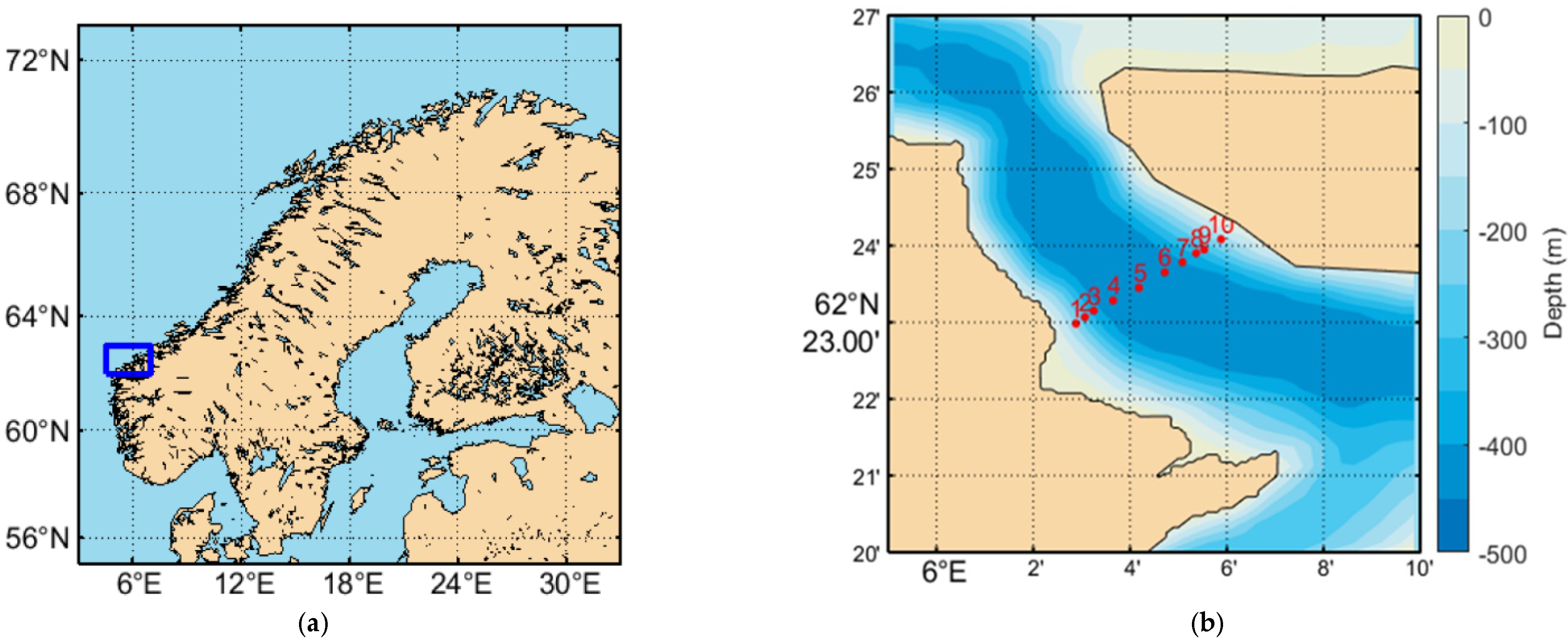
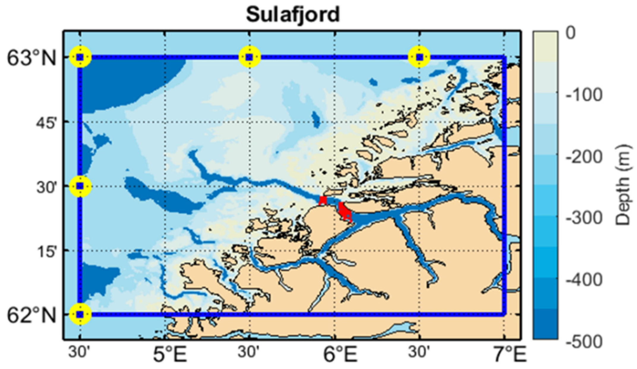
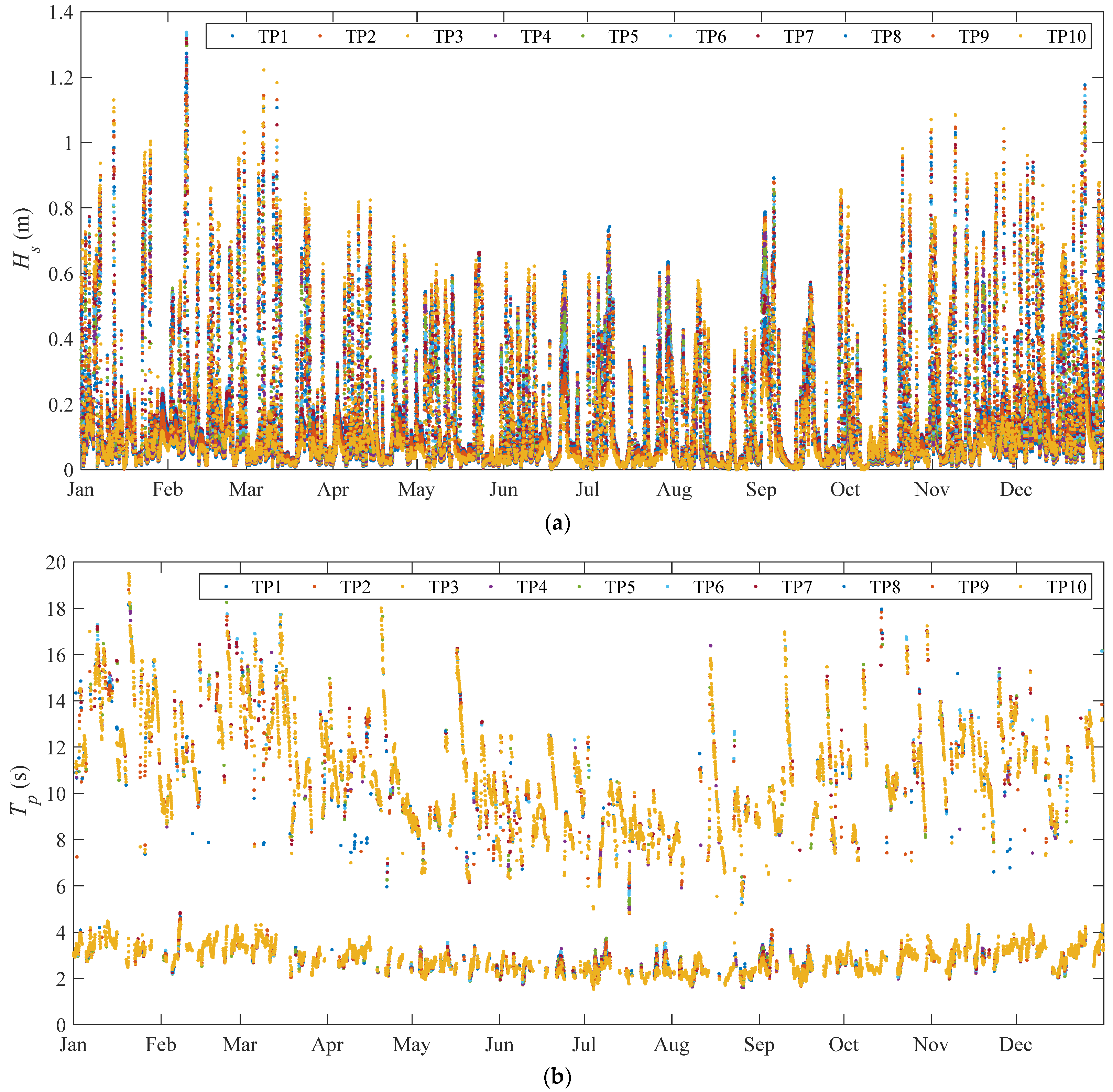
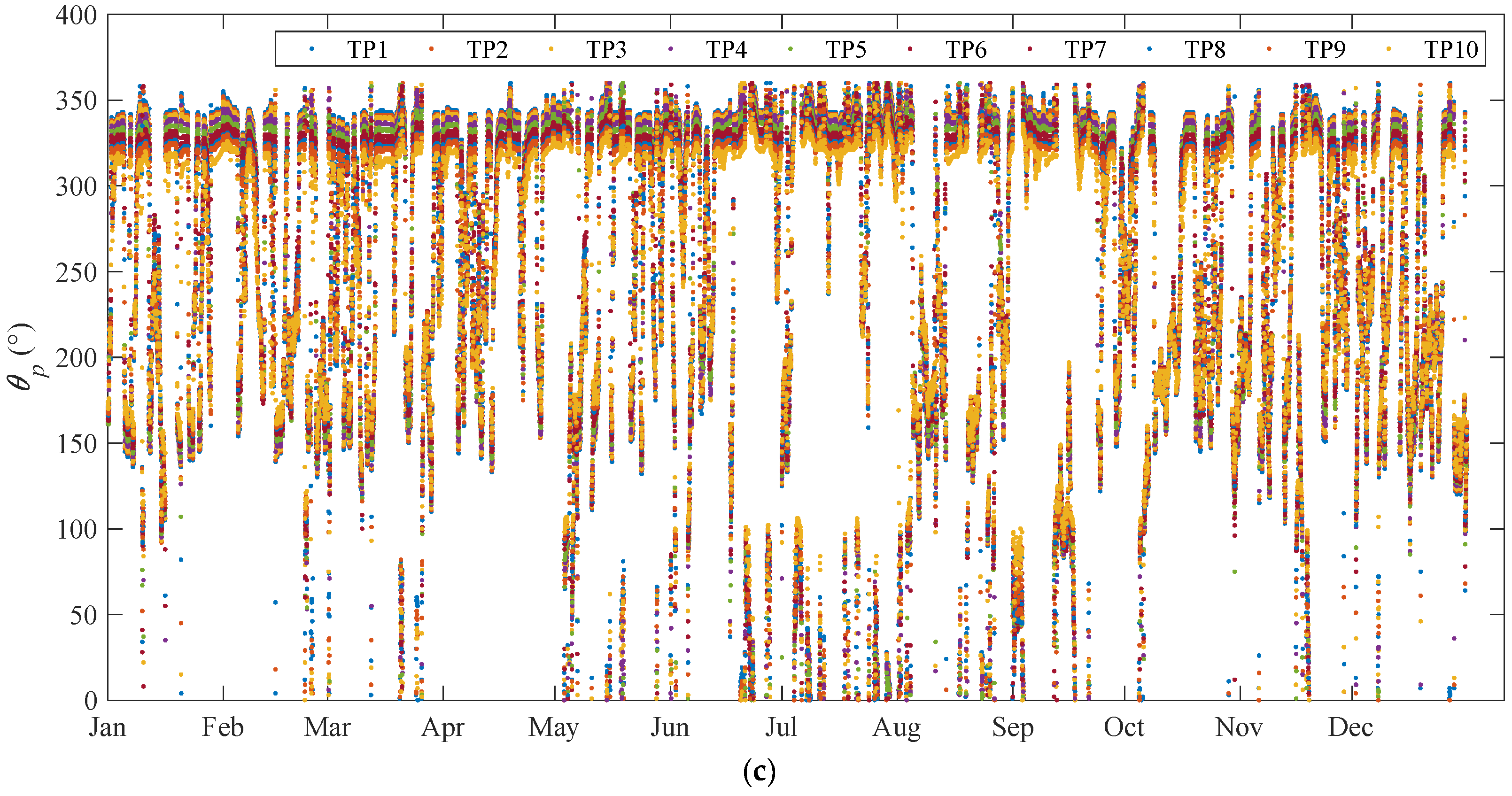
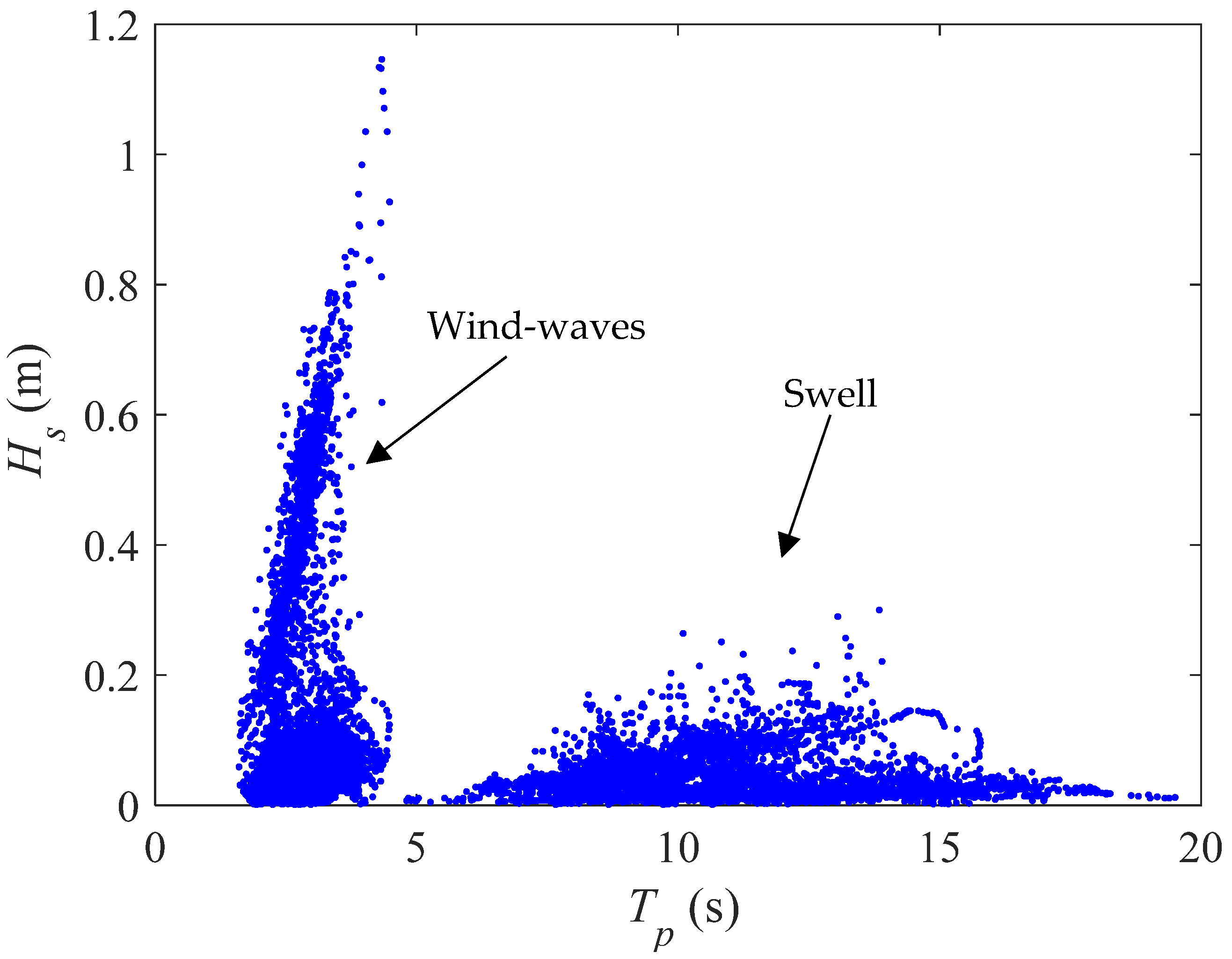
In this paper, a computational study of the dynamic response of a long, straight and side-anchored floating bridge under inhomogeneous wave conditions is carried out. A hypothetical crossing at the Sulafjord is chosen, and the wave environment in the year 2015 at 10 positions along the crossing is numerically computed. Next, different inhomogeneous wave conditions are established based on the wave data at 3, 5, and 10 positions, respectively. Time-domain simulations are conducted to examine the effect of different modelling approaches of the inhomogeneous wave conditions on the global responses of a long, straight, and side-anchored floating bridge.

This paper is organized as follows: Section 2 defines the problem and describes the models used in this study. Section 3 presents and discusses the results of the inhomogeneous sea states at the selected site location. The global analysis of a long floating bridge considering different modelling approaches of the inhomogeneous wave condition is presented in Section 4. Concluding remarks are given in Section 5.

2. Models and Methods

In this study, a hypothetical crossing at the Sulafjord is selected for numerical simulation and analysis of the inhomogeneous wave field. Then, an inhomogeneous wave condition is established, and a series of inhomogeneous wave load cases are defined based on different modelling approaches. Next, the effect of different inhomogeneous wave load cases on a long, straight, and side-anchored floating bridge design concept for the crossing of the Bjørnafjord is examined.

2.1. Selected Site Location and Enviromental Modelling

A hypothetical crossing in the area of the Sulafjord, central Norway, is considered in this study. Figure 1 shows the selected site location of the crossing. The total length of the crossing is approximately 4250 m. Ten positions along the crossing, marked TP1 to TP10, are selected for analysis of the inhomogeneous sea states. The coordinates of the ten positions are listed in

Table 1. Coordinates and water depth of 10 positions along the crossing.

Position	Longitude			Latitude			Depth
	Degree	Minute	Second	Degree	Minute	Second	m
TP1	6	2	53	62	22	59	234
TP2	6	3	4	62	23	4	329
TP3	6	3	15	62	23	9	368
TP4	6	3	39	62	23	17	419
TP5	6	4	11	62	23	27	441
TP6	6	4	43	62	23	39	436
TP7	6	5	5	62	23	47	403
TP8	6	5	22	62	23	54	350
TP9	6	5	32	62	23	57	304
TP10	6	5	53	62	24	5	161

. It should be emphasized that this location is chosen in view of the fact that the wave field in the Sulafjord was found to be inhomogeneous [9] and the crossing length is very similar to that at the Bjørnafjord where a floating bridge is planned to be constructed [14,15].

Figure 2 illustrates the procedure for the sea environment simulation and generation of the inhomogeneous wave conditions for the current study. Wave data from the well-known climatology of ECMWF ERA5 [26] is used as input to the numerical analysis of the inhomogeneous wave conditions at the selected hypothetical crossing. In the present study, the data from 2010 to 2015 with a 1 h interval is used. SWAN is employed with detailed bathymetry of the modelled area for the numerical analysis of the environmental conditions at the selected 10 positions along the hypothetical crossing. Figure 3 shows the modelled region with five yellow points representing the boundaries where the input of wave data is available. The in-between points of the boundary take interpolated values. At the shore boundaries, waves are not generated, and the land absorbs all incoming wave energy. The environmental model covers a planar area of 1 degree in latitude by 2.5 degrees in longitude. A refined resolution of 150 m is adopted for a nested area of 15 km by 15 km that covers the hypothetical crossing. The outputs include the hourly wave spectra at the ten selected locations along the hypothetical crossing, using 34 frequencies and 36 directions. For more detailed information of the environmental modelling, reference is made to [17,27]. Note that the accuracy of the SWAN model was validated by comparison with field measurement data [17,27]. The calculated wave spectra are next processed by selecting the most severe wave conditions in one year and fitted to the wave conditions at the Bjørnafjord by keeping the wave characteristics (significant wave height H_s, peak period T_p and mean wave direction θ_p) while adopting the spectral parameters (non-dimensional peak parameter γ and spreading coefficient n) specified in the design basis [28]. This is discussed in detail in Section 2.3 and Section 3.

2.2. Floating Bridge Model

An idealized straight and side-anchored floating bridge model based on the phase 3 design concept for the crossing of the Bjørnafjord [29,30] is employed in this study to investigate the effect of inhomogeneous wave conditions on the global bridge responses. Figure 4 illustrates the bridge model with a total span length of 4.6 km. In view of the fact that both the Bjørnafjord crossing and the hypothetical crossing at the Sulafjord are sufficiently deep to assume deepwater conditions [31], the water depth is set to a constant value of 300 m in the numerical model. The bridge girder is vertically supported by 35 pontoons, labeled A1 to A35, with an even spacing of 125 m. The bridge is laterally restrained by four mooring clusters spaced approximately 1 km apart. Each mooring cluster is tethered to a moored pontoon and composed of eight mooring lines arranged in a semi-taut configuration. Each mooring line contains a top studless chain segment of 50 m, an intermediate spiral strand wire segment of 600 m, and a bottom studless chain segment of 50 m. The nominal diameter, dry mass per unit length, and axial stiffness for chain segments are 147 mm, 432.2 kg/m, and 1.73 × 10⁶ kN, respectively [29,30]. Likewise, these quantities are 124 mm, 80.3 kg/m, and 1.42 × 10⁶ kN, respectively, for wire segments [29,30].

Table 2. Sectional properties of bridge girder and column sections. I_x’ denotes the torsional constant. I_y’ and I_z’ refer to the second moment of inertia about the local y’- and z’-axes. I_x’x’ is the mass moment of inertia per unit length about x’ axis.

Property	H1	S1	F1	C
Mass	17,530 kg/m	19,780 kg/m	16,040 kg/m	9180 kg/m
Area	1.38 m2	1.65 m2	1.17 m2	1.53 m2
Ix’	5.79 m4	7.88 m4	6.64 m4	14.92 m4
Iy’	2.87 m4	4.06 m4	3.21 m4	9.65 m4
Iz’	107.22 m4	116.52 m4	89.88 m4	12.94 m4
Ix’x’	1.2 × 106 kg/m∙m2	1.3 ×106 kg/m∙m2	1.1 × 106 kg/m∙m2	2.3 × 105 kg/m∙m2

lists the sectional properties of the bridge girders and columns.

Table 3. Pontoon properties.

Property	Moored Pontoon	Unmoored Pontoon
Weight (ton)	1452	850
Height (m)	8.5	5
Displacement (m3)	5.7 × 103	3.3 × 103
Roll inertia (ton m2)	4.2 × 105	2.2 × 105
Pitch inertia (ton m2)	6.1 × 104	2.3 × 104
Yaw inertia (ton m2)	4.2 × 105	2.3 × 105
Heave stiffness (kN/m)	6.7 × 103	6.7 × 103
Roll stiffness (kNm/rad)	1.5 × 106	1.5 × 106
Pitch stiffness (kNm/rad)	8.9 × 104	8.9 × 104

lists the pontoon properties. Note that both moored and unmoored pontoons have the same planar dimensions as shown in Figure 4. Moored pontoons have a larger height and thus a larger draft to allow for a larger water displacement to counterbalance the vertical forces exerted by the mooring lines. The boundary conditions are summarized in

Table 4. Boundary conditions.

Degree of Freedom	South End	North End
Translation x	Restrained	Released
Translation y	Restrained	Restrained
Translation z	Restrained	Restrained
Rotation x	Restrained	Restrained
Rotation y	Restrained	Restrained
Rotation z	Restrained	Released

. Note that the longitudinal translation and rotation about the vertical axis are released at the north end to allow for thermal expansion and contraction as well as easy connection to the transitional bridge [29].

The finite element method is employed for numerical representation of the superstructure and the mooring systems of the floating bridge physical model. More specifically, the bridge girders and columns are modelled using Euler beam elements accounting for pure torsion in view of their slenderness. The mooring lines are modelled using compressionless bar elements. The bridge pontoons are modelled as rigid bodies attached to the lower ends of the bridge columns. The structural damping is modelled by using Rayleigh damping with a 0.5% damping ratio for the lowest two vibration modes for the steel structures [28]. Note that in the calculation of structural damping, the effect of added mass due to the fluid is not accounted for. In addition to the structural damping, potential damping and viscous drag due to the sea water, as discussed below, are also included in the global floating bridge model.

Both the mooring lines and the bridge pontoons are subjected to wave-induced hydrodynamic loads. For the submerged part of the mooring lines, the hydrodynamic load per unit length is evaluated by using the Morison equation as

$$f_m={\rho }_{w}V{\dot{u}}_m+{\rho }_w{C}_{a}V\left({\dot{u}}_w-{\dot{u}}_m\right)+\frac{1}{2}{\rho }_w{C}_{d}D\left(u_w-u_m\right)\left|u_w-u_m\right|$$

(1)

Herein, ρ_w is the water density, V is the volume per unit length of the mooring line, D is the diameter of the mooring line, C_a is the added mass coefficient, and C_d is the quadratic drag coefficient.

Table 5. Morison coefficients for mooring lines.

Coefficients	Chain	Wire
Ca	1.0	1.0
Cd longitudinal	1.5	0.1
Cd transverse	2.4	2.4

lists the coefficients for chain and wire segments. u_m is the velocity of the mooring line, while u_w is the flow speed. The over-dots denote the time derivative, i.e., the accelerations of the mooring line (${\dot{u}}_m$) and the water flow (${\dot{u}}_w$).

WAMIT is employed to calculate the added mass, potential damping, and wave excitation force transfer functions of the bridge pontoons in the frequency domain. The hydrodynamic coupling between adjacent pontoons is neglected as the spacing is considered to be large enough. By applying the Cummins formulation, the governing equations of motion for a bridge pontoon can be written as

$${\displaystyle \sum _{j=1}^6\left(M_p+A_j^{\infty }\right){\ddot{u}}_{pj}\left(t\right)}+{\displaystyle {\int }_{-\infty }^{\infty }{\kappa }_j\left(t-\tau \right){\dot{u}}_{pj}\left(t\right)d\tau }+\left(K_j^h+K_j^b\right)u_{pj}\left(t\right)=F_j^{exc}\left(t\right)$$

(2)

where M_p is the pontoon mass, A_j^∞ is the added mass corresponding to the jth degree of the freedom at infinite frequency, κ_j is the retardation function, K_j^h represents the hydrostatic restoring stiffness, K_j^b is the stiffness from the adjacent bridge structure, u_pj is the relevant displacement component of the pontoon, and F_j^exc is the excitation force. Note that the effect of second-order difference-frequency wave excitation force components was examined in detail in [14] and was found to be negligible in all global bridge responses except for the transverse displacement of the bridge girder. Similar observations were reported in studies on long fjord-crossing floating bridges [32,33]. Thus, only the first-order wave excitation forces are considered in this study.

The full bridge model is constructed and analyzed using the commercial software package SIMA through a coupled SIMO-RIFLEX solver.

Table 6. Lowest modes of floating bridge model.

Mode Number	Period	Dominating Axis	Mode Shape
1	33.8 s	y
2	30.9 s	y
3	30.1 s	y
7	11.6 s	x
41	7.2 s	z

lists the first few modes of the bridge model as well as the model shape of the girder. Note that this bridge model has been verified earlier [14,15], and the modal properties agree well with those reported in the independent reference reports [29,30].

2.3. Modelling Inhomogeneous Waves

The modelling of inhomogeneous wave loads is based on the assumption that the sea state around any arbitrary pontoon can be regarded as being homogeneous, while the spatial variations of the wave characteristics along the crossing is represented by considering different sea states at different pontoon locations [10,11,12,13,14,15]. This is deemed reasonable in view of the fact that the pontoon dimensions are much smaller than the spacing between adjacent pontoons. The homogeneous wave condition at a given position may be characterized by a unidirectional wave spectrum S(ω) and a directional spreading function D(θ) as

$$S\left(\omega \right)=\frac{5}{16}\left(1-0.287\ln \left(\gamma \right)\right)H_s^2\frac{{\omega }_p^4}{{\omega }^5}{e}^{-\frac{5}{4}{\left(\frac{\omega }{{\omega }_p}\right)}^{-4}}{\gamma }^{-\frac{1}{2}{\left(\frac{\omega -{\omega }_p}{\sigma {\omega }_p}\right)}^2}$$

(3)

$$D\left(\theta \right)=\frac{\Gamma \left(1+\frac{n}{2}\right)}{\sqrt{\pi }\Gamma \left(\frac{1}{2}+\frac{n}{2}\right)}{\cos }^n\left(\theta -{\theta }_p\right)$$

(4)

where γ is the non-dimensional peak parameter, Hs is the significant wave height, ω is the angular wave frequency, ω_p is the peak angular frequency, σ is the spectrum width parameter and is 0.07 when ω ≤ ω_p and 0.09 when ω > ω_p, θ is the wave heading, θ_p is the mean wave heading, and n is the spreading coefficient. In this study, γ and n are set to 2.3 and 4, respectively [28].

As stated earlier, the inhomogeneous wave conditions along a hypothetical crossing at the Sulafjord are first investigated numerically using SWAN. Next, the inhomogeneous wave conditions are applied to the floating bridge model. As the two crossing lengths for the Sulafjord versus the Bjørnafjord are slightly different, the relative distances between the 10 selected positions along the hypothetical crossing are spatially upscaled such that the total crossing length matches the length of the bridge model.

Table 7. Mapping of 10 selected positions to nearest bridge pontoons.

Selected Positions	Pontoon Number
TP1	A3
TP2	A5
TP3	A7
TP4	A10
TP5	A15
TP6	A20
TP7	A24
TP8	A27
TP9	A28
TP10	A31

provides information about the mapping of the 10 positions to the nearest bridge pontoons. The wave conditions at other pontoon locations are obtained based on a linear interpolation. As the SWAN model is based on phase-averaged energy balance equations, the information of the phase difference between wave components is lost. In this study, two conditions are considered. The first refers to fully coherent and correlated waves where the random phase angle of each wave component is identical at all pontoon locations. The second condition refers to completely uncorrelated waves at different pontoon locations by assigning different random phase angles to each pontoon location.

3. Inhomogeneous Wave Conditions and Load Cases

Based on the model and the input data described in Section 2.1, the wave conditions along the hypothetical crossing numerically analyzed. It should be highlighted that there are field measurement data at three buoy locations along the crossing available for the period between April 2017 and July 2019. A comparison between the numerical analysis using the SWAN model and field measurement of the wave conditions was carried out and a good agreement was found [17,27], thereby implying that the employed SWAN model is reliable.

3.1. Analysis of Wave Conditions

Statistical analysis is conducted to provide a description of the wave conditions along the hypothetical crossing. Figure 5 shows the significant wave height H_s, wave peak period T_p, and mean wave heading θ_p at the selected 10 positions for the year 2015. Note that the presented statistical results are calculated based on 1 h intervals. Moreover, note that only the results corresponding to year 2015 are presented owing to the page constraint. As it can be seen in Figure 5, waves are harsher in the winter period. The maximum H_s is slightly above 1.3 m, which is very close to that of the annual maximum sea state at the Bjørnafjord. The peak periods span widely between 1.6 s and 20 s. Clearly, wind waves and swells co-exist at the hypothetical crossing. It should be highlighted that the mean wave headings θ_p are presented according to the nautical convention, i.e., the direction where the waves come from is measured clockwise from geographic North. The results show that the wave heading is primarily within 330–350°, which indicates that the waves are mainly propagating into the fjord when it is read in conjunction with Figure 1b.

Figure 6 further plots the scatter diagram of the significant wave height H_s and peak period T_p at TP1 throughout the year 2015. The peak periods of wind waves vary between 1.6 s and 4.4 s. In general, wind waves with a higher H_s are associated with a longer T_p. For swells, the wave peak period can reach 19.5 s. However, the corresponding significant wave heights are mostly below 0.3 m, which is quite a small value, and the energy is expected to be very low as compared to the wind waves. This is supported by a similar study reported in [14]. Thus, only wind waves are considered in the following studies.

A further examination of the results reveals that the maximum significant wave heights for wind waves occur simultaneously at the ten selected positions along the hypothetical crossing. These extreme values are considered as the characteristics of the representative annual maximum sea states at the crossing and utilized to establish an inhomogeneous wave condition. Figure 7 shows the spatial variation along the crossing of the significant wave height, peak period and mean wave direction. Note that the mean wave directions are presented according to the nautical convention, i.e., 0 refers to the waves from the North. As it can be seen, there is a special variation of H_s along the crossing with the highest value occurring at TP6. The inhomogeneity in T_p is relatively small except at TP10 where a substantial drop is observed. Similarly, the mean wave direction is mostly between 320° and 350°, and a significant change is found at TP10.

3.2. Establishing Inhomogeneous Wave Load Cases

The wave characteristics at the hypothetical crossing at the Sulafjord are quite similar to the annual design values at the Bjørnafjord where the construction of a floating bridge is planned [28]. Thus, these sea states are suitable for further detailed structural analysis of the floating bridge model. As one of the main focuses of the study is to investigate the effect of different resolutions adopted in modelling inhomogeneous wave conditions on the global bridge responses, different numbers of data points along the hypothetical crossing will be used to establish different inhomogeneous wave load cases. According to the wave inhomogeneity presented in Figure 7, the selection of data points is made based on the spatial variation of H_s along the crossing. Three different selections of data points are considered in this study. Wave load case 1 (LC1) is established based on the wave conditions at TP1, TP6, and TP10. These three locations represent the two ends and an intermediate position at pontoon location A20 where the most severe sea state is observed. They correspond to the bridge pontoon locations A3, A20, and A31, respectively (see Table 6). Wave load case 2 (LC2) builds upon LC1 with two more data points (TP4 and TP8). Wave load case 3 (LC3) is established utilizing all ten data points along the crossing, which serves as the reference for comparation with the other two wave load cases.

Figure 8 shows the spatial variations of the wave characteristics at different bridge pontoon locations. Note that mean wave direction shown in Figure 8 is adjusted according to the coordinate systems illustrated in Figure 4. As it can be seen, LC1 employing the three-point approach is able to represent the spatial variation of H_s quite well. However, substantial discrepancies are observed for T_p and θ_p after A20. LC2 employing the five-point approach is found to match LC3 closely. Only small deviations between A1 and A8 and A20 and between A22 and A29 are observed for T_p and after A27 for θ_p.

Each inhomogeneous wave load case is further composed of two sub-load cases. The first sub-load case assumes a fully coherent and correlated wave field, and the second assumes a completely uncorrelated, random wave field.

Table 8. Description of wave load cases.

Wave Load Case	Representation of Wave Inhomogeneity	Wave Correlation
LC1.1	3-point approach	Fully correlated
LC1.2	3-point approach	Uncorrelated
LC2.1	5-point approach	Fully correlated
LC2.2	5-point approach	Uncorrelated
LC3.1	10-point approach	Fully correlated
LC3.2	10-point approach	Uncorrelated

lists all the wave load cases considered in this study. Note that for each wave load case, five independent wave seeds are run for a simulation length of 1 h for each seed, and the average values are used to reduce the statistical uncertainties. This is expected to be sufficient in view of results of a similar study reported in [15]. In total, there are 30 individual simulations.

4. Structural Responses of Floating Bridge

Time domain simulations are conducted to investigate the bridge responses corresponding to the different inhomogeneous wave load cases as listed in Table 8. The dynamic responses along the bridge girder are focused upon in the present study. In order to concentrate on the effect of employing different inhomogeneous wave modelling approaches, this study excludes the effect of other environmental loads such as current and wind loads. The traffic load is also excluded.

To examine the statistical uncertainty associated with the employment of five 1 h simulations,

Table 9. Statistic transverse displacement of girder at pontoon location A18.

Statistical Results		1 h Simulation						5 h
		Seed 1	Seed 2	Seed 3	Seed 4	Seed 5	Average
Max	Value	0.0767 m	0.0878 m	0.0891 m	0.0842 m	0.0713 m	0.0818 m	0.0891 m
	Difference	13.92%	1.46%	0.00%	5.50%	19.98%	8.19%	−
SD	Value	0.0194 m	0.0192 m	0.0199 m	0.0199 m	0.0199 m	0.0197 m	0.0197 m
	Difference	1.52%	2.53%	−1.02%	−1.02%	−1.02%	0.20%	−

lists the maximum values (Max) and standard deviations (SD) of the transverse displacement of the bridge girder at pontoon location A18 under a fully correlated inhomogeneous wave condition modelled by the 10-point approach. This point is purposely chosen in view of the fact that large displacement is expected around the mid-point of the floating bridge. The mean values are not examined in view of the fact that they are virtually zero. The statistical values computed from each of the five seeds and their averages are compared with the compiled equivalent 5 h simulation. Note that the equivalent 5 h simulation is a compilation of the data from the five 1 h simulations. As it can be seen, the relative differences due to 1 h simulations are limited, and the use of their averages can effectively reduce the statistical uncertainties.

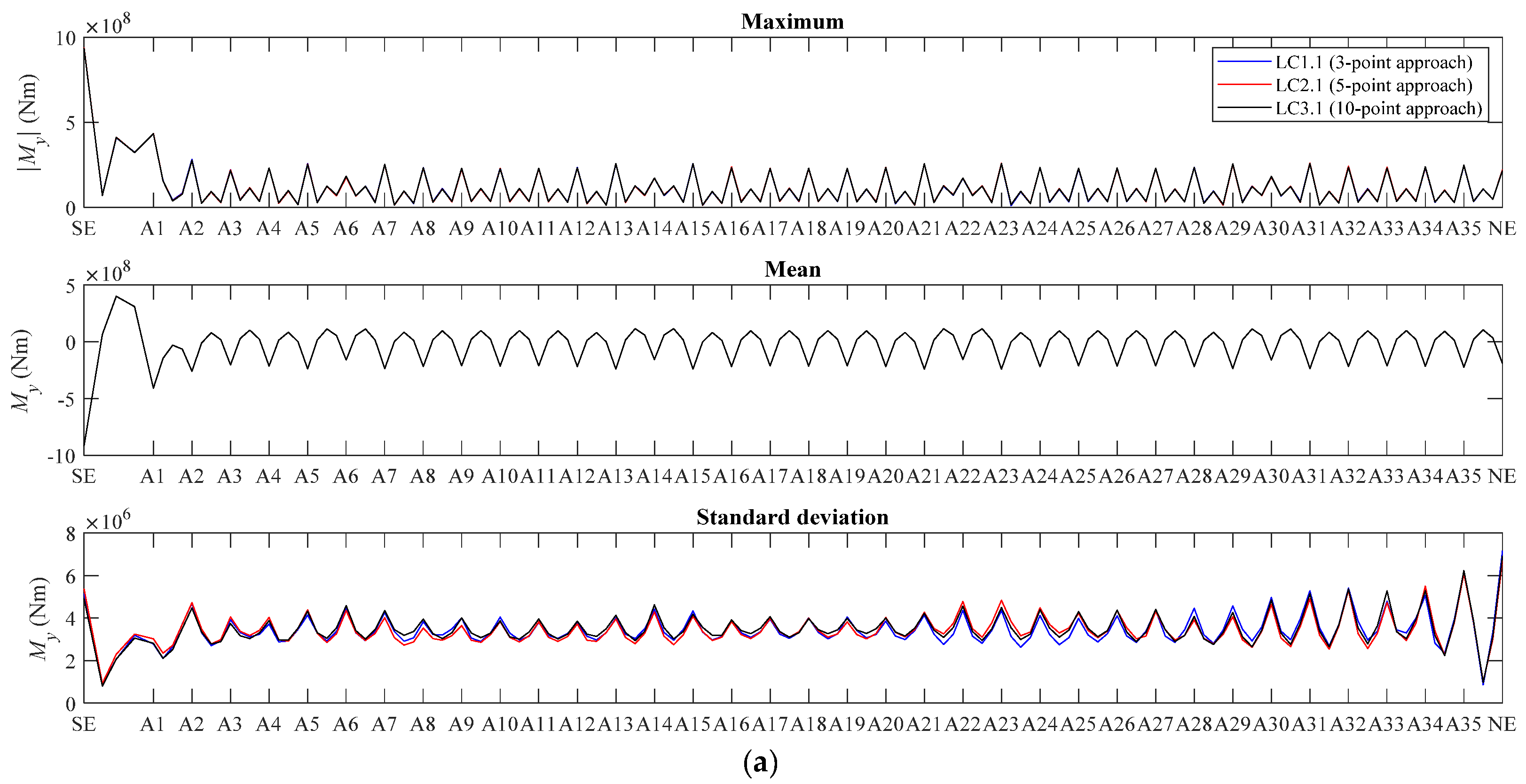
Figure 9 and Figure 10 show the statistical results for the bending moments along the bridge girder about the global y- and z-axes, respectively. As it can be seen, there are some small discrepancies in the standard deviations of M_y between the three fully correlated wave load cases. The maximum discrepancy is found to occur within the segment between A23 and A25. It is slightly reduced to 10% when the waves are uncorrelated. It is also observed that the different modelling approaches mainly introduce local discrepancies, while the global maxima are rather similar. The differences in the maximum and mean values are found to be negligible. This is expected as they are dominated by the self-weight of the bridge girder. However, it should be highlighted that the discrepancies in the standard deviations may affect the prediction of fatigue damage in the bridge girder [15]. As for M_z, the modelling approaches affect both the maximum values and the standard deviations. The discrepancies are found to be within 33% and 10% for the maximum values and standard deviations, respectively, when the waves are fully correlated. The maximum discrepancies are slightly reduced to 30% and 9% for the maximum values and the standard deviations, respectively, when the waves are uncorrelated. Similar to M_y, the global maxima predicted by using the three different approaches are close to each other despite of the local discrepancies.

Figure 11 shows the statistical results of the girder’s torsional moment. As it can be seen, both the maximum torsion values and the standard deviations are affected by different inhomogeneous wave modelling approaches. The 3-point approach tends to underestimate both the standard deviations and the maximum values. The discrepancies associated with the standard deviations are within 12% for fully correlated wave load cases and reduce to 8% for uncorrelated wave load cases. The different modelling approaches have greater effects on the maximum torsions of the bridge girder. The maximum discrepancies are found to be 25% and 26% for fully correlated and uncorrelated wave load cases, respectively. The 5-point approach is found to generate results that are in a good agreement with the 10-point approach.

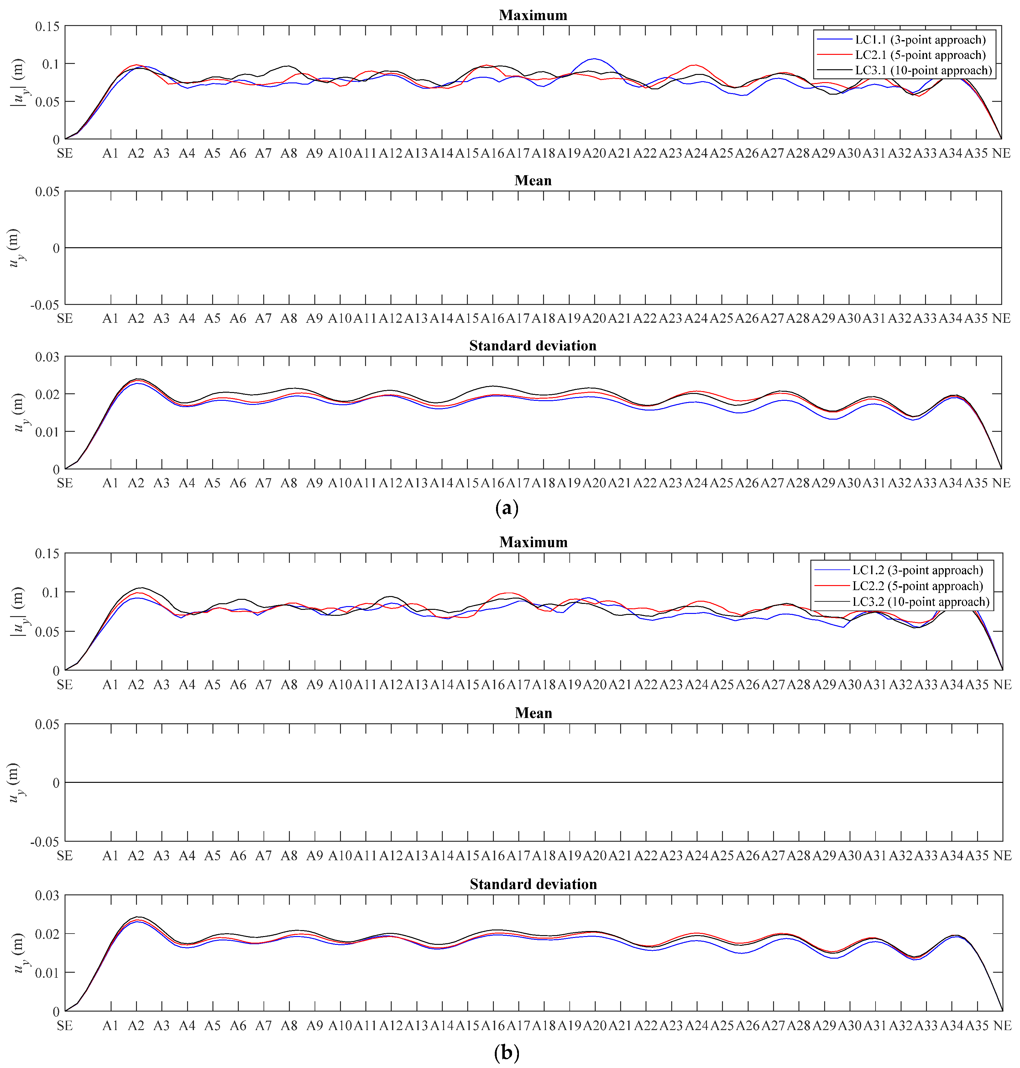
Figure 12 and Figure 13 show the motion statistics along the bridge girder for the y- and z-displacement components, respectively. In general, the discrepancies in the standard deviations for the transverse displacement along the girder are within 12% for both correlated and uncorrelated wave load cases. The 3-point approach tends to underestimate the standard deviations throughout the entire bridge length, while the 5-point approach substantially reduces the discrepancy, especially for the segment between A22 and the north end. The discrepancies in the maximum transverse displacement are found to be within 23% and 20%, respectively, for the correlated and uncorrelated wave load cases. Owing to the self-weight of the bridge, the different modelling approaches are found to have virtually no effect on the maximum and mean values of the vertical displacement of the girder. However, large discrepancies are observed for the standard deviations of the vertical displacement, especially for the segment between A22 and A29. Within this segment, the 3-point approach leads to underestimated responses while the 5-point approach overestimates the dynamic motion. Apparently, the differences in both T_p and θ_p have a substantial influence on the dynamic vertical motion responses of the bridge girder. Beyond this segment, both 3-point and 5-point approaches tend to slightly underestimate the vertical motion responses. It is also observed that the discrepancies are reduced when the waves are uncorrelated.

5. Conclusions

In this paper, the dynamic response of a long, straight, and side-anchored floating bridge under inhomogeneous wave loads is investigated. A hypothetical crossing at the Sulafjord is chosen, and the wave environment at 10 selected positions along the crossing is numerically analyzed. Next, different inhomogeneous wave conditions are established based on selected wave data at 3, 5, and 10 positions, respectively. Time-domain simulations are conducted to examine the effect of different modelling approaches of the inhomogeneous wave condition on the global responses of a floating bridge.

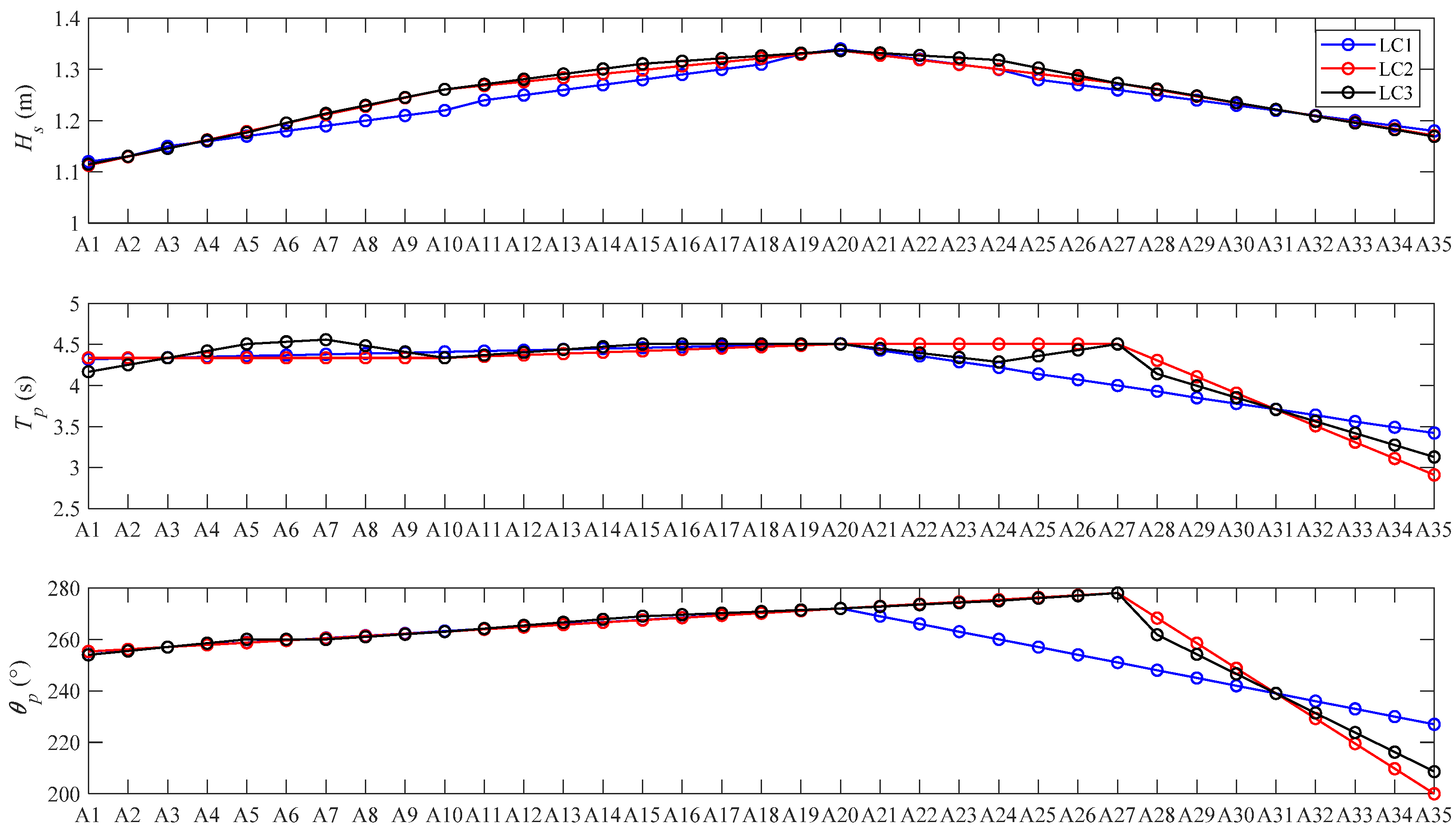
The analysis of the wave field along a hypothetical crossing at the Sulafjord shows that the spatial wave inhomogeneities vary gradually. This implies that it may be possible to model the inhomogeneous wave field by using a reduced resolution in the numerical simulation for the sake of computational efficiency. Three different inhomogeneous wave conditions based on a selection of different numbers of data points are thus established, and a total of six wave load cases are defined.

The global structural analysis of the floating bridge girder shows that different modelling approaches introduce a little difference in the global maxima of the bending moment and motions. This implies that it may be possible to employ a simplified and coarser model for the inhomogeneous wave conditions in a preliminary bridge analysis. This could potentially result in a reduction in the number of inhomogeneous wave conditions to consider in the study and thus reduce the computational cost. However, attention should be paid to local regions in connection with detailed analysis and design as local discrepancies in both bending moment and girder motions are observed. Furthermore, different modelling approaches are found to result in discrepancies in the standard deviations of the girder’s responses. They may lead to different fatigue damage estimations which could affect the bridge design. It is also observed that the 3-point approach tends to underestimate the torsion in the bridge girder. The discrepancies for uncorrelated wave load cases are generally smaller than those for coherent and fully correlated wave load cases.

References

1. The E39 Coastal Highway Route. Available online: https://www.vegvesen.no/en/roads/Roads+and+bridges/Road+projects/e39coastalhighwayroute (accessed on 21 February 2021).
2. Holand, I.; Sigbjörnsson, R.; Langen, I. Dynamic analysis of a curved floating bridge. In IABSE Proceedings; ETH Zurich: Zurich, Switzerland; p. 5/77.
3. Langen, I.; Sigbjörnsson, R. On stochastic dynamics of floating bridges. Eng. Struct. 1980, 2, 209–216. [Google Scholar] [CrossRef]
4. Langen, I. Probabilistic methods for dynamic analysis of floating bridges. Norweg. Marit. Res. 1983, 11, 2–15. [Google Scholar]
5. Leira, B.J.; Langen, I. On probabilistic design of a concrete floating bridge. Nord. Concr. Res. 1984, 3, 140–166. [Google Scholar]
6. Hartz, B. Dynamic response of the hood-canal floating bridge. In Second ASCE/EMD Specialty Conference on Dynamic Response of Structures; American Society of Civil Engineers: Atlanta, CA, USA, 1981. [Google Scholar]
7. Seif, M.S.; Inoue, Y. Dynamic analysis of floating bridges. Mar. Struct. 1998, 11, 29–46. [Google Scholar] [CrossRef]
8. Cheng, Z.; Svangstu, E.; Gao, Z.; Moan, T. Field measurements of inhomogeneous wave conditions in Bjørnafjorden. J. Waterw. Port Coast. Ocean Eng. 2019, 145, 05018008. [Google Scholar] [CrossRef] [Green Version]
9. Lie, H.; Fu, S.; Fylling, I.; Fredriksen, A.G.; Bonnemaire, B.; Kjersem, G.L. Numerical modelling of floating and submerged bridges subjected to wave, current and wind. In Proceedings of the 35th International Conference on Ocean, Offshore and Arctic Engineering, OMAE’2016, Busan, Korea, 19–24 June 2016. [Google Scholar]
10. Wei, W.; Fu, S.; Moan, T.; Lu, Z.; Deng, S. A discrete-modules-based frequency domain hydroelasticity method for floating structures in inhomogeneous sea conditions. J. Fluid. Struct. 2017, 74, 321–339. [Google Scholar] [CrossRef]
11. Wei, W.; Fu, S.; Moan, T.; Song, C.; Ren, T. A time-domain method for hydroelasticity of very large floating structures in inhomogeneous sea conditions. Mar. Struct. 2018, 57, 180–192. [Google Scholar] [CrossRef]
12. Cheng, Z.; Gao, Z.; Moan, T. Wave load effect analysis of a floating bridge in a fjord considering inhomogeneous wave conditions. Eng. Struct. 2018, 163, 197–214. [Google Scholar] [CrossRef]
13. Ding, J.; Tian, C.; Wu, Y.; Wang, X.; Liu, X.; Zhang, K. A simplified method to estimate the hydroelastic responses of VLFS in the inhomogeneous waves. Ocean Eng. 2019, 172, 434–445. [Google Scholar] [CrossRef]
14. Dai, J.; Leira, B.J.; Moan, T.; Kvittem, M.I. Inhomogeneous wave load effects on a long, straight and side-anchored floating pontoon bridge. Mar. Struct. 2020, 72, 102763. [Google Scholar] [CrossRef]
15. Dai, J.; Leira, B.J.; Moan, T.; Alsos, H.S. Effect of wave inhomogeneity on fatigue damage of mooring lines of a side-anchored floating bridge. Ocean Eng. 2021, 219, 108304. [Google Scholar] [CrossRef]
16. Fylling, I.J. Dynamisk Analyse av Flytebrukonsept for Sulesund—Hareid. MARINTEK Report 580319. 2012. Available online: https://ntnuopen.ntnu.no/ntnu-xmlui/handle/11250/237050 (accessed on 13 May 2021).
17. Stefanakos, C.N.; Furevik, B.R.; Knutsen, Ø.; Christakos, K. Nearshore wave modelling in a Norwegian fjord. In Proceedings of the 39th International Conference on Ocean, Offshore and Arctic Engineering, OMAE’2020 Virtual, Online, 3–7 August 2020. [Google Scholar]
18. Cheng, Z.; Svangstu, E.; Moan, T.; Gao, Z. Assessment of inhomogeneity in environmental conditions in a Norwegian fjord for design of floating bridges. Ocean Eng. 2021, 220, 108474. [Google Scholar] [CrossRef]
19. The WAMDI Group. The WAM model-A third generation ocean wave prediction model. J. Phys. Oceanogr. 1998, 18, 1775–1810. [Google Scholar]
20. Tolman, H. A third-generation model for wind waves on slowly varying, unsteady, and inhomogeneous depths and currents. J. Phys. Oceanogr. 1991, 21, 782–797. [Google Scholar] [CrossRef]
21. Booij, N.; Ris, R.; Holthuijsen, L. A third-generation wave model for coastal regions: 1. model description and validation. J. Geophys. Res. Sect. Ocean. 1999, 104, 7649–7666. [Google Scholar] [CrossRef] [Green Version]
22. Engsig-Karup, A.P.; Madsen, M.G.; Glimberg, S.L. A massive parallel gpu-accelerated model for analysis of fully nonlinear free surface waves. Int. J. Numer. Methods Fluids 2012, 70, 20–36. [Google Scholar] [CrossRef] [Green Version]
23. Wang, W.; Bihs, H.; Kamath, A.; Arntsen, Ø. Large scale CFD modelling of wave propagation in Sulafjord for the E39 project. In Proceedings of the 9th National Conference on Computational Mechanics, MekIT’2017, Trondheim, Norway, 11–12 May 2017. [Google Scholar]
24. Sørensen, O.; Kofoed-Hansen, H.; Rugbjerg, M.; Sørensen, L. A third generation spectral wave model using an unstructured finite volume technique. In Proceedings of the 29th International Conference of Coastal Engineering, Lisbon, Portugal, 19–24 September 2004; pp. 894–906. [Google Scholar]
25. Massey, T.C.; Anderson, M.E.; Smith, J.M.; Gomez, J.; Jones, R. STWAVE: Steady-State Spectral Wave Model User’s Manual for STWAVE, Version 6.0; Technical Report; U.S. Army Corps of Engineers; Engineer Research and Development Center; Coastal and Hydraulics Laboratory: Vicksburg, MI, USA, 2011. [Google Scholar]
26. ERA5. Available online: https://www.ecmwf.int/en/forecasts/datasets/reanalysis-datasets/era5 (accessed on 21 February 2021).
27. Stefanakos, C.; Dai, J.; Leira, B. Investigation of inhomogeneous wave conditions in Sulafjorden. In Proceedings of the 31st International Ocean and Polar Engineering Conference, Rhodes, Greece, 20–25 June 2021. (accepted). [Google Scholar]
28. Vegvesen Statens. SBJ-32-C3-SVV-90-BA-002 Design Basis Bjørnafjorden Rev; E. Statens Vegvesen: Oslo, Norway, 2018.
29. Multiconsult. SBJ-31-C3-MUL-22-RE-100-0—Analysis and Design (Base Case); Multiconsult AS: Oslo, Norway, 2017. [Google Scholar]
30. DNV GL. SBJ-31-C3-DNV-62-RE-018-0 Bjørnafjorden Side Anchored Floating Bridge—Independent Global Analyses; DNV GL: Oslo, Norway, 2018. [Google Scholar]
31. Cheng, Z.; Gao, Z.; Moan, T. Hydrodynamic load modeling and analysis of a floating bridge in homogeneous wave conditions. Mar. Struct. 2018, 59, 122–141. [Google Scholar] [CrossRef]
32. Viuff, T.; Leira, B.J.; Xiang, X.; Øiseth, O. Effects of wave directionality on extreme response for a long end-anchored floating bridge. Appl. Ocean Res. 2019, 90, 101843. [Google Scholar] [CrossRef]
33. Viuff, T.; Xiang, X.; Øiseth, O.; Leira, B.J. Model uncertainty assessment for wave-and current-induced global response of a curved floating pontoon bridge. Appl. Ocean Res. 2020, 105, 102368. [Google Scholar] [CrossRef]
Figure 1. Selected hypothetical crossing: (a) global view; (b) zoomed-in view with 10 positions along the crossing selected for analysis.
Jmse 09 00548 g001
Figure 2. Flowchart of generating inhomogeneous wave conditions.
Jmse 09 00548 g002
Figure 3. Domain of the modelled region.
Jmse 09 00548 g003
Figure 4. Floating bridge model.
Jmse 09 00548 g004
Figure 5. Significant wave height (a), peak wave period (b), and mean wave heading according to nautical convention (c) at 10 selected positions.
Jmse 09 00548 g005aJmse 09 00548 g005b
Figure 6. Scatter plot of Tp and Hs at TP1 throughout year 2015.
Jmse 09 00548 g006
Figure 7. Inhomogeneous wave condition ((a) Hs, (b) Tp and (c) θp according to nautical convention) at the hypothetical crossing.
Jmse 09 00548 g007
Figure 8. Inhomogeneous wave condition (Hs, Tp and θp according to bridge coordinate) at the hypothetical crossing.
Jmse 09 00548 g008
Figure 9. Bending moment about the y-axis along the bridge girder: (a) correlated waves and (b) uncorrelated waves.
Jmse 09 00548 g009aJmse 09 00548 g009b
Figure 10. Bending moment about the z-axis along the bridge girder: (a) correlated waves and (b) uncorrelated waves.
Jmse 09 00548 g010
Figure 11. Torsional moment along bridge girder: (a) correlated waves and (b) uncorrelated waves.
Jmse 09 00548 g011
Figure 12. Transverse displacement along bridge girder: (a) correlated waves and (b) uncorrelated waves.
Jmse 09 00548 g012
Figure 13. Vertical displacement along bridge girder: (a) correlated waves and (b) uncorrelated waves.
Jmse 09 00548 g013