
Unsteady Linearisation of Bed Shear Stress for Idealised Storm Surge Modelling

 , , , and
Abstract
:1. Introduction
- Equation (2) can be applied locally, leading to an r-value valid at a single point in the model domain. However, to facilitate analytical solution, the friction coefficient r is often assumed to be spatially uniform over the model domain (or over subdomains); the energy criterion introduced above should then be applied in a spatially integrated sense. This implies that Equation (2) must be replaced with a more complex expression, involving spatial and tidal averaging; also see Section 2.
- The solution to the hydrodynamic problem, consisting of flow velocity and surface elevation as functions of space and time, obviously depends on the friction coefficient r. However, the solution also depends on the velocity amplitude U through Equation (2) and thus again on the solution itself, since U is also a flow variable. This cyclic dependency can be tackled by an iterative procedure that converges to an r-value for which U agrees with the velocity amplitude of the solution. We argue that, when allowing for , the ‘linear’ stress parametrisation in Equation (2) is in fact still nonlinear in u.
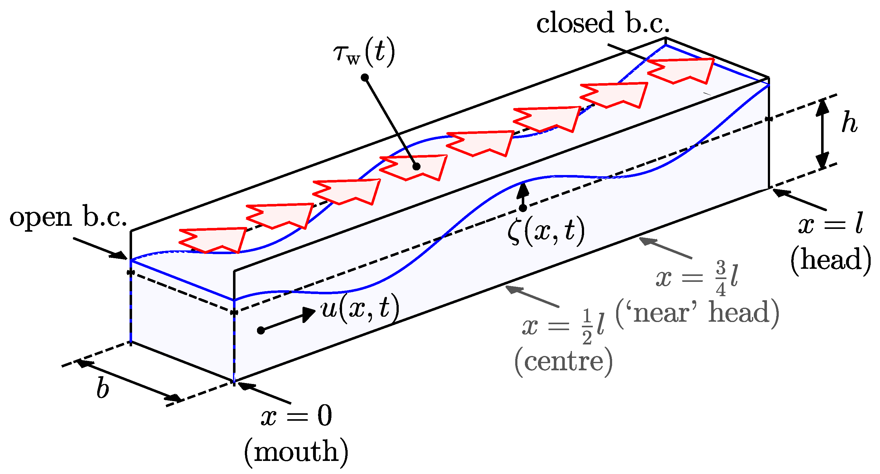
2. Model Formulation
3. Solution Procedure
3.1. Model Development
3.2. Fourier Expansion
3.3. Iterative Procedure
- Define an initial function of the friction coefficient , e.g., zero or some other constant function, and determine the associated Fourier coefficients .
- Find the surface elevation by solving Equation (9) in Fourier space. Since and are known, this problem is linear in the unknown complex amplitude functions . We solve it using matrix algebra (details in Appendix A.1).
- Obtain the flow velocity by applying Equation (5). This provides the Fourier coefficients (see Appendix A.2).
- Substitute in Equation (7) to obtain an updated friction coefficient . The integrals therein are evaluated on an equidistant grid with N points in the x-direction, using the trapezoidal rule. This step also produces new Fourier coefficients .
- Verify whether and satisfy the convergence criterionwith user-defined convergence tolerance . If so, the instantaneous power criterion is satisfied with sufficient precision over the entire simulation time, the current solution is converged in the sense of the second caveat on equivalent linearisations in Section 1, and the procedure is completed.
- If Equation (11) is not satisfied, apply relaxation to find the next guess for the friction coefficient: , with a relaxation parameter that can be tuned to accelerate convergence. Then, repeat the procedure from step 2 onward using the new function and the associated Fourier coefficients .
3.4. Procedure for the Steady Friction Coefficient
3.5. Reference Finite-Difference Solution with Quadratic Bed Shear Stress
4. Results
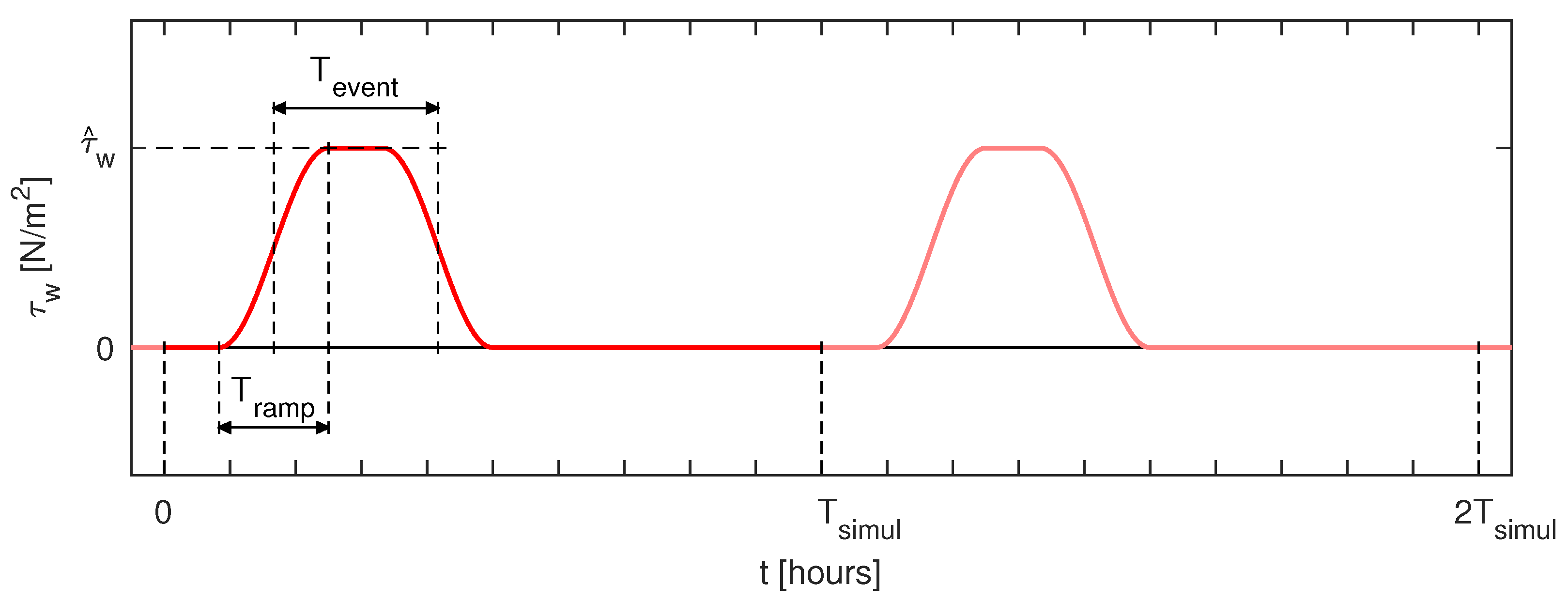
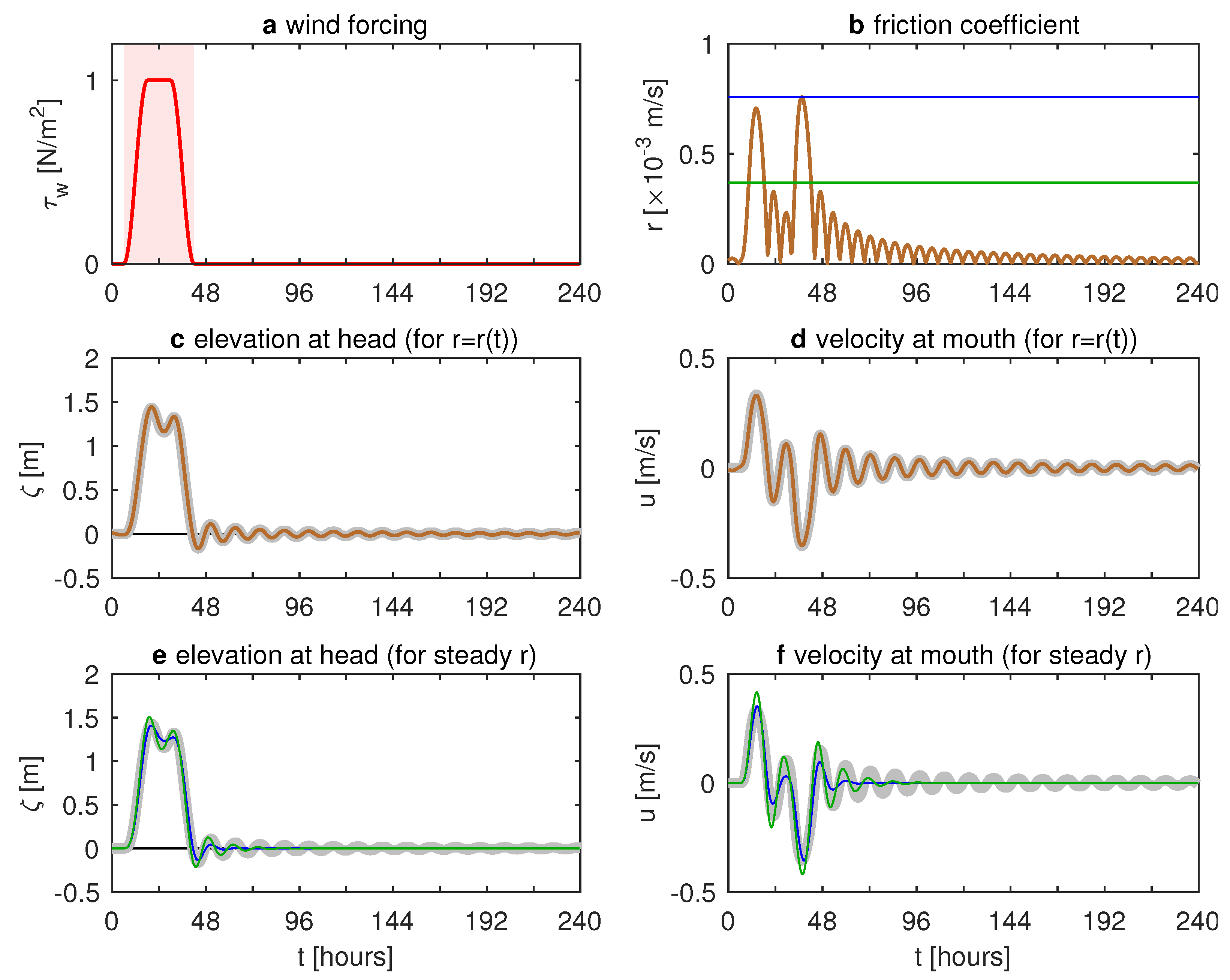
4.1. Wind Forcing Only: Synthetic Storm Event
4.2. Wind and Tide Forcing
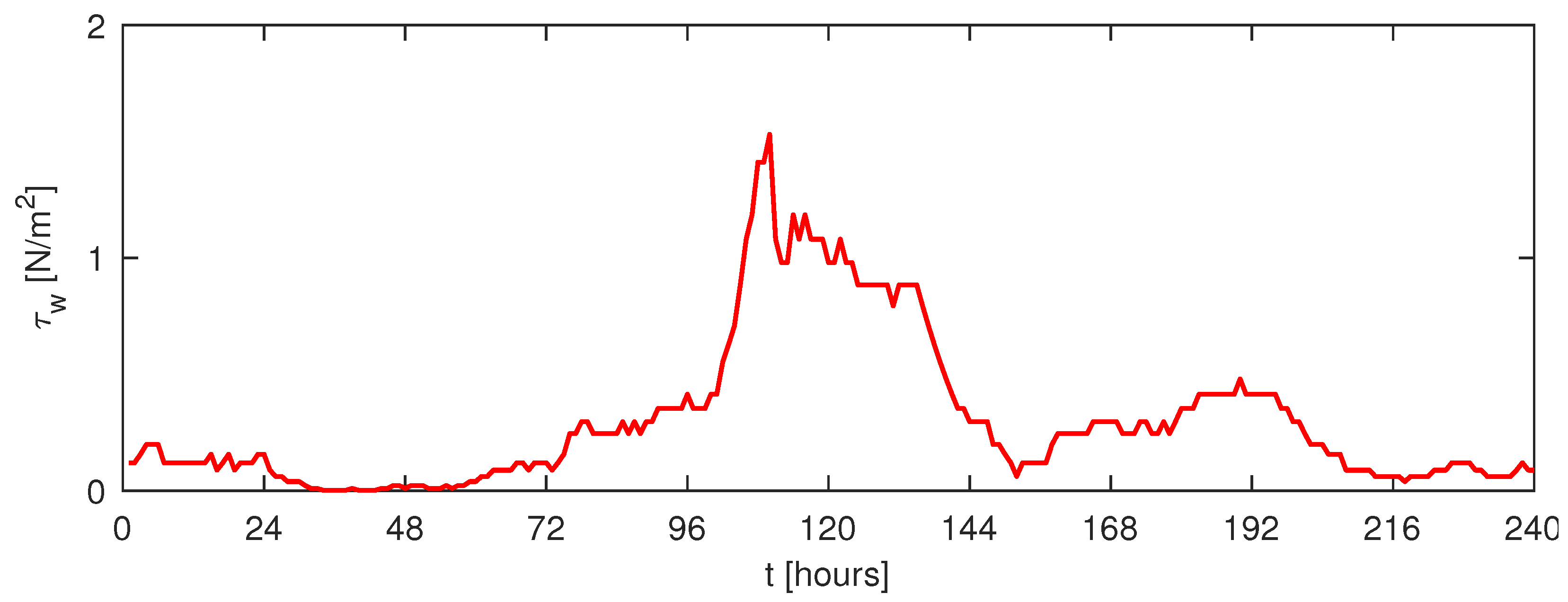
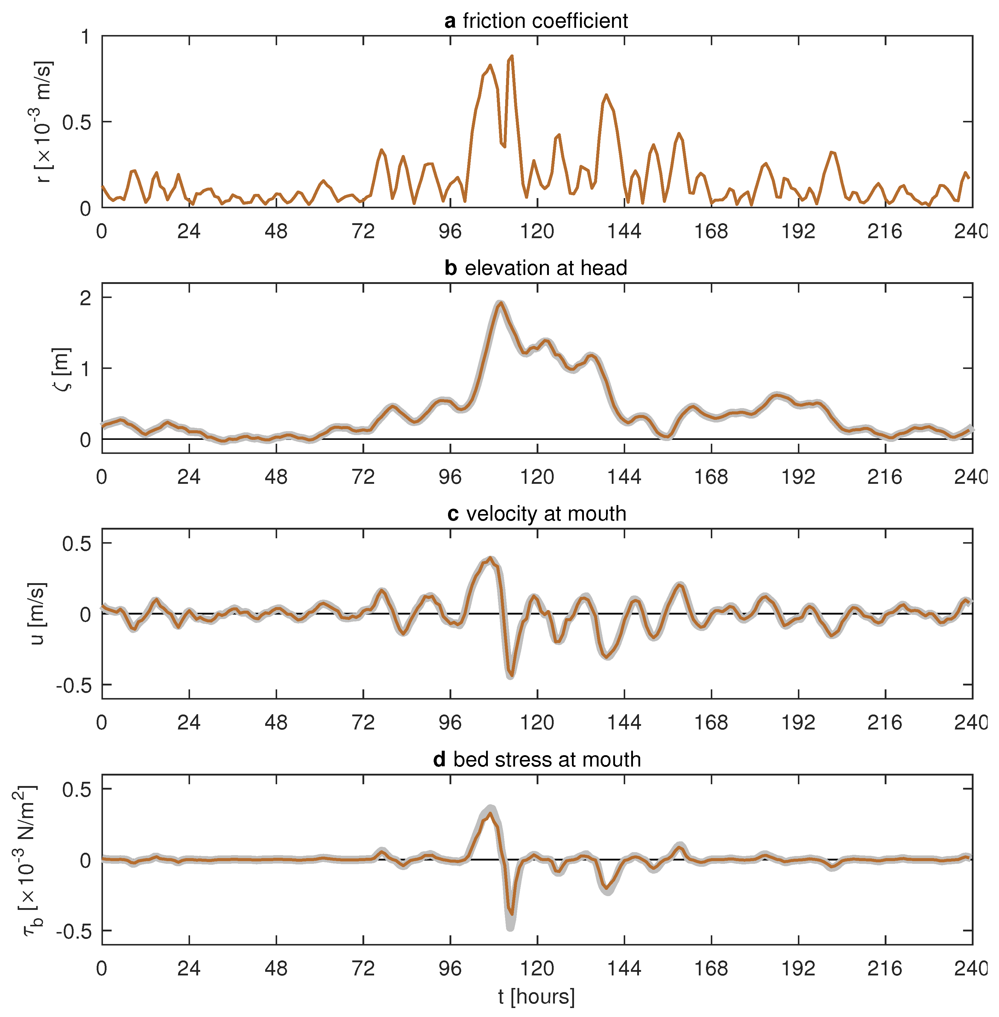
4.3. Realistic Wind Forcing
5. Discussion
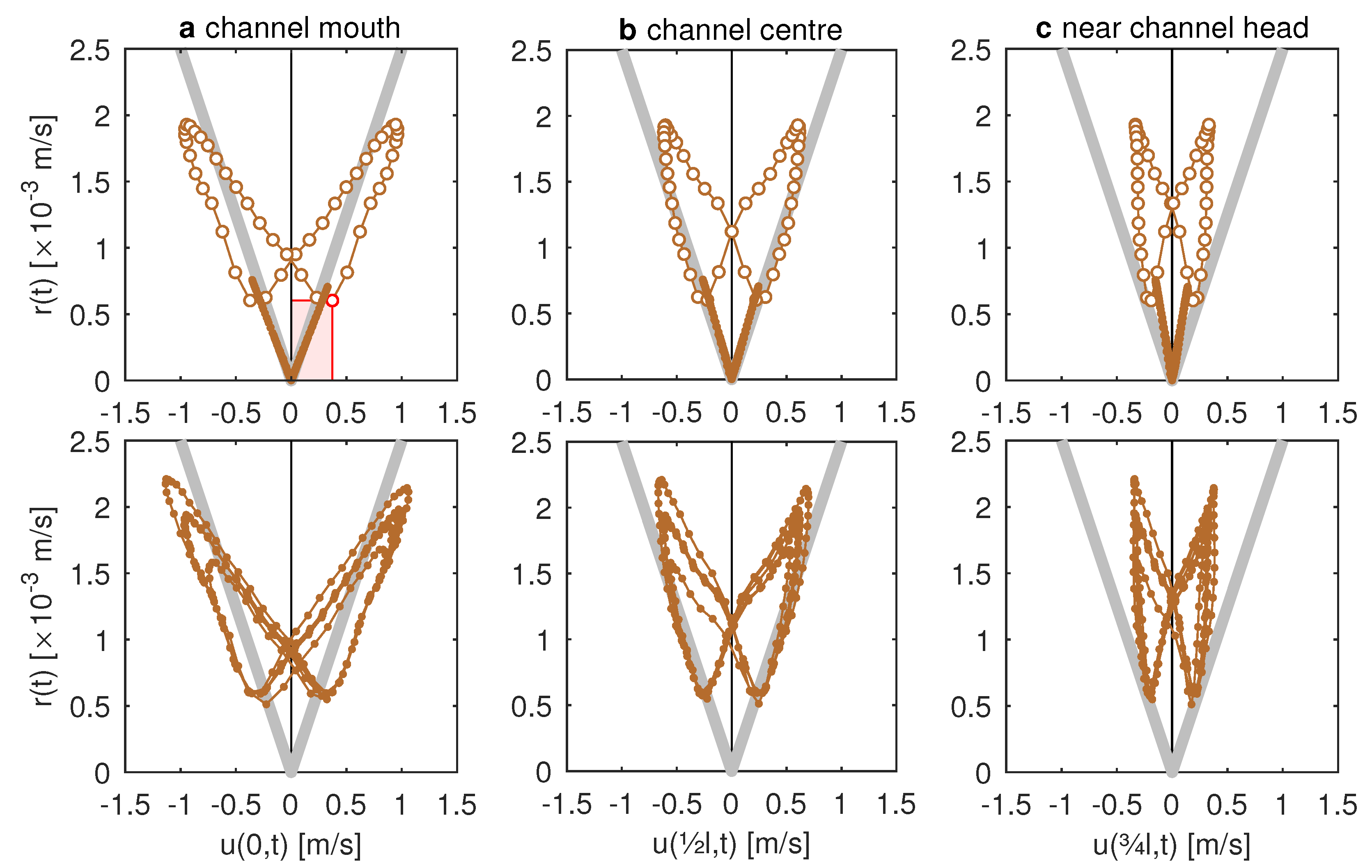
- For the wind-only simulations, closely follows the quadratic parametrisation, as shown by the V-shaped arrangement of the data points in the top of Figure 8;
- For the tide-only simulations, follows an oscillatory path and the continuous presence of nonzero currents inside the channel prevents it from approaching zero;
- Finally, for wind-tide simulations, the path of -values is similar to the combined path for wind and tide forcing but is additionally deformed by the tide-surge interactions.
6. Conclusions
Author Contributions
Funding
Data Availability Statement
Conflicts of Interest
Appendix A. Details of the Solution Procedure
Appendix A.1. Step 1: Surface Elevation
Appendix A.2. Step 2: Flow Velocity
Appendix B. Scaling Analysis
References
- Pugh, D.T.; Woodworth, P.L. Sea-Level Science. Understanding Tides, Surges, Tsunamis and Mean Sea-Level Changes; Cambridge University Press: Cambridge, UK, 2014. [Google Scholar]
- Prandle, D.; Wolf, J. The interaction of surge and tide in the North Sea and River Thames. Geophys. J. R. Astr. Soc. 1978, 55, 203–216. [Google Scholar] [CrossRef] [Green Version]
- Horsburgh, K.J.; Wilson, C. Tide-surge interaction and its role in the distribution of surge residuals in the North Sea. J. Geophys. Res. 2007, 112, C08003. [Google Scholar] [CrossRef] [Green Version]
- Murray, A.B. Contrasting the goals, strategies, and predictions associated with simplified numerical models and detailed simulations. In Predictions in Geomorphology; Geophysical, M., Iverson, R.M., Wilcock, P.R., Eds.; AGU: Washington, DC, USA, 2003; Volume 135, pp. 151–165. [Google Scholar]
- Lorentz, H.A. Het in rekening brengen van den weerstand bij schommelende vloeistofbewegingen. De Ingenieur 1922, 37, 695. [Google Scholar]
- Lorentz, H.A. Verslag van de Staatscommissie Zuiderzee 1918–1926; Technical Report; Algemeene Landsdrukkerij: Den Haag, The Netherlands, 1926. [Google Scholar]
- Mei, C.C. The Applied Dynamics of Ocean Surface Waves; World Scientific: Singapore, 1989. [Google Scholar]
- Zimmerman, J.T.F. On the Lorentz linearization of a nonlinearly damped tidal Helmholtz oscillator. Proc. Kon. Ned. Akad. v. Wetensch. 1992, 95, 127–145. [Google Scholar]
- Roos, P.C.; Velema, J.J.; Hulscher, S.J.M.H.; Stolk, A. An idealized model of tidal dynamics in the North Sea: Resonance properties and response to large-scale changes. Ocean Dyn. 2011, 61, 2019–2035. [Google Scholar] [CrossRef] [Green Version]
- Hulscher, S.J.M.H.; de Swart, H.E.; de Vriend, H.J. The generation of offshore tidal sand banks and sand waves. Cont. Shelf Res. 1993, 13, 1183–1204. [Google Scholar] [CrossRef] [Green Version]
- Terra, G.M.; van de Berg, W.J.; Maas, L.R.M. Experimental verification of Lorentz’ linearization procedure for quadratic friction. Fluid Dyn. Res. 2005, 36, 175–188. [Google Scholar] [CrossRef] [Green Version]
- Jeffreys, H. The Earth: Its Origin, History and Physical Constitution, 5th ed.; Cambridge University Press: Cambridge, UK, 1970. [Google Scholar]
- Inoue, R.; Garrett, C. Fourier Representation of Quadratic Friction. J. Phys. Oceanogr. 2007, 37, 593–610. [Google Scholar] [CrossRef]
- Chen, W.L.; Roos, P.C.; Schuttelaars, H.M.; Hulscher, S.J.M.H. Resonance properties of a closed rotating rectangular basin subject to space- and time-dependent wind forcing. Ocean Dyn. 2015, 65, 325–339. [Google Scholar] [CrossRef] [Green Version]
- Chen, W.L.; Roos, P.C.; Schuttelaars, H.M.; Kumar, M.; Zitman, T.J.; Hulscher, S.J.M.H. Response of large-scale coastal basins to wind forcing: Influence of topography. Ocean Dyn. 2016, 66, 549–565. [Google Scholar] [CrossRef] [Green Version]
- Reef, K.R.G.; Lipari, G.; Roos, P.C.; Hulscher, S.J.M.H. Time-varying storm surges on Lorentz’s Wadden Sea networks. Ocean Dyn. 2018, 68, 1051–1065. [Google Scholar] [CrossRef] [Green Version]
- Pitzalis, C. Time-Dependent Linearized Friction: A Development on Lorentz’ Energy Argument. Master’s Thesis, Civil Engineering & Management, University of Twente, Enschede, The Netherlands, 2017. [Google Scholar]


| Parameter | Symbol | Value | Unit |
|---|---|---|---|
| Water depth | h | 8 | |
| Channel length | l | 100 | |
| Drag coefficient (bottom friction) | - | ||
| Drag coefficient (wind stress) | - | ||
| Gravitational acceleration | g | ||
| Water density | 1000 | ||
| Air density | |||
| Duration of storm event | 24 | ||
| Ramp-up time (equal to ramp-down time) | 12 | ||
| Peak value of wind stress | 1 | ||
| Tidal period | 12 | ||
| Tidal elevation amplitude | 1 | ||
| Truncation number of Fourier series in Equation (10) | M | 512 | - |
| Simulation period | 240 | ||
| Relaxation parameter | - | ||
| Number of points in space to evaluate power criterion | N | 240 | - |
| Convergence tolerance | |||
| Space step | |||
| Time step | 60 |
Publisher’s Note: MDPI stays neutral with regard to jurisdictional claims in published maps and institutional affiliations. |
© 2021 by the authors. Licensee MDPI, Basel, Switzerland. This article is an open access article distributed under the terms and conditions of the Creative Commons Attribution (CC BY) license (https://creativecommons.org/licenses/by/4.0/).
Share and Cite
Roos, P.C.; Lipari, G.; Pitzalis, C.; Reef, K.R.G.; Campmans, G.H.P.; Hulscher, S.J.M.H. Unsteady Linearisation of Bed Shear Stress for Idealised Storm Surge Modelling. J. Mar. Sci. Eng. 2021, 9, 1160. https://0-doi-org.brum.beds.ac.uk/10.3390/jmse9111160
Roos PC, Lipari G, Pitzalis C, Reef KRG, Campmans GHP, Hulscher SJMH. Unsteady Linearisation of Bed Shear Stress for Idealised Storm Surge Modelling. Journal of Marine Science and Engineering. 2021; 9(11):1160. https://0-doi-org.brum.beds.ac.uk/10.3390/jmse9111160
Chicago/Turabian StyleRoos, Pieter C., Giordano Lipari, Chris Pitzalis, Koen R. G. Reef, Gerhardus H. P. Campmans, and Suzanne J. M. H. Hulscher. 2021. "Unsteady Linearisation of Bed Shear Stress for Idealised Storm Surge Modelling" Journal of Marine Science and Engineering 9, no. 11: 1160. https://0-doi-org.brum.beds.ac.uk/10.3390/jmse9111160