Environmental Kuznets Curve Hypothesis on CO₂ Emissions: Evidence for China

Abstract

China is the largest CO₂ emitter in the world, and it shared 28% of the global CO₂ emissions in 2017. According to the Paris Agreement, it is estimated that China’s CO₂ emissions will reach its peak by 2030. However, whether or not the CO₂ emissions in China will rise again from its peak is still unknown. If the emission level continues to increase, the Chinese policymakers might have to introduce a severe CO₂ reduction policy. The aim of this paper is to conduct an empirical analysis on the long-standing relationship between CO₂ emissions and income while controlling energy consumption, trade openness, and urbanization. The autoregressive distributed lag (ARDL) model and the bounds test were adopted in evaluating the validity of the Environmental Kuznets Curve (EKC) hypothesis. The quantile regression was also used as an inference approach. The study reveals two major findings: first, instead of the conventional U-shaped EKC hypothesis, there is the N-shaped relationship between CO₂ emissions and real gross domestic product (GDP) per capita in the long run. Second, a positive effect of energy consumption and a negative effect of urbanization on CO₂ emissions, in the long run, are also estimated. Quantitatively, if energy consumption rises by 1%, then CO₂ emissions will increase by 0.9% in the long run. Therefore, the findings suggest that a breakthrough, in terms of policymaking and energy innovation under China’s specific socioeconomic and political circumstances, are required for future decades.

1. Introduction

Nowadays, rapid environmental degradation and modern infrastructure development are causing critical challenges to human life (Aguila 2020). Huge economic growth is, in one way or another, related to fossil fuel consumption, which contributes toward warming the atmosphere by producing massive greenhouse gases (GHGs) in the environment (Hanaki and Portugal-Pereira 2018; Toma et al. 2020). GHG production is considered the main factor that influences carbon dioxide (CO₂) emissions (Abeydeera et al. 2019).

In order to control CO₂ emissions and other pollutants, there has been greater concern in China for more efficient environmental regulations, energy innovation, and multilateral environmental agreements. China’s 13th five-year plan, to promote the reduction of its gross domestic product (GDP) per unit of energy consumption by 15% by 2020, as well as the depletion of its GDP per unit of CO₂ emissions by at least 40% by 2020, is compared to the levels in 2015. Meanwhile, according to the Paris Agreement, China promised to reach its peak CO₂ emissions no later than 2030. Consequently, there is a need for a more thorough study on the output-emission nexus in China as the guidebook for policymakers to adopt appropriate measures and achieve these targets.

Changes in the environment and the impact of the gig economy means that environment policymakers have changed their decision to sustain the gig economy (and contribution to the environment). China witnessed its unprecedented economic boom during the last 40 years, since the 1978 reforms. According to the International Monetary Fund (IMF), in terms of purchasing-power-parity, China continues to be the largest economy in the world after surpassing the U.S. in 2014 (Monaghan 2014; Boumphrey 2014). Due to economic growth, China has been the largest CO₂ emitter since 2008 (Shan et al. 2018), and it shared 28% of the global CO₂ emission in 2017, as reported by the International Energy Agency (IEA). In this circumstance, there is a need for effective analysis to identify the relationship between CO₂ emissions and income.

In 2015, China’s non-fossil energy consumption accounted for around 12.4% of its total primary energy consumption, as reported by IEA in the World Energy Balances. According to the Copenhagen Accord, China’s 2020 targets are to set its carbon intensity about −40% to −45% below 2005 and to increase its non-fossil share of total energy supply to 15%. The carbon intensity goal was achieved ahead of time when China’s carbon intensity declined by 4.0% in 2018 and by 45.8% cumulatively compared to 2005, as reported by the National Bureau of Statistics of China in 2019. On September 3, 2016, China ratified the Paris commitments through the nationally determined contribution (NDC) submitted to the United Nations Framework Convention on Climate Change (UNFCCC). In the NDC, China promised to peak its CO₂ emissions and to expand its proportion of non-fossil energy supply to 20% by 2030. To achieve these goals, pilot carbon markets have been enacted in the Shanghai municipality and Guangdong province in China, which, since 2013, have continued to refine the market rules and mechanisms.

The Chinese government also launched the national emissions trading system (ETS) in December 2017. The national ETS began with the power generation sector in 2018, and once certain criteria are met, other sectors will be gradually covered (Slater et al. 2019). Moreover, an allocation of CO₂ emissions allowance was initiated to the power sector on September 30, 2019, as a trial policy, according to the Chinese Ministry of Ecology and Environment. Despite the efforts, the Chinese government is aiming to accomplish all of the plans mentioned in the above climate accords for GHG emissions. There is a need to overcome some challenges, such as the large-scale geographical differences in China. Furthermore, Wang et al. (2019) emphasized that China’s 2017 ETS should develop features that are different from other national ETSs in the world, due to its unique social and political background.

The nexus between environmental degradation and the economy has been a major area of concern in recent years and has become an important topic in environmental economics. The negative impact on natural ecosystems in wealthier and emerging economies, as a result of environmental degradation, has been reported (Sannigrahi et al. 2019, 2020; Mosconi et al. 2020; Porrini 2017). Articles (Grossman and Krueger 1991; Shafik and Bandyopadhyay 1992; Grossman and Krueger 1995; Holtz-Eakin and Selden 1995); it was concluded that air and water pollutant emissions increase with economic output initially, and decline after reaching a certain threshold value. This pattern of environmental degradation is denoted by the Environmental Kuznets Curve (EKC) hypothesis, which indicates that environmental quality deteriorates at first when income is at low levels, but ameliorates with income at high levels.

The relationship between economic activity and environmental damage is affected by the policy framework, regulating the limits of activities concerning non-desirable outputs of the production. This is especially true for China, where a great state transformation took place within the period considered by the present study, the policy regulation is very relevant in affecting growth and environmental protection. China went through sequential phases to reforms and introduced a severe CO₂ reduction policy (Naughton 2008; Brandt et al. 2014). Several researchers broadly analyzed the CO₂ emissions growth and income relationship by observing China’s reforms policy, with an eye on the time series data, as well as historic emission patterns.

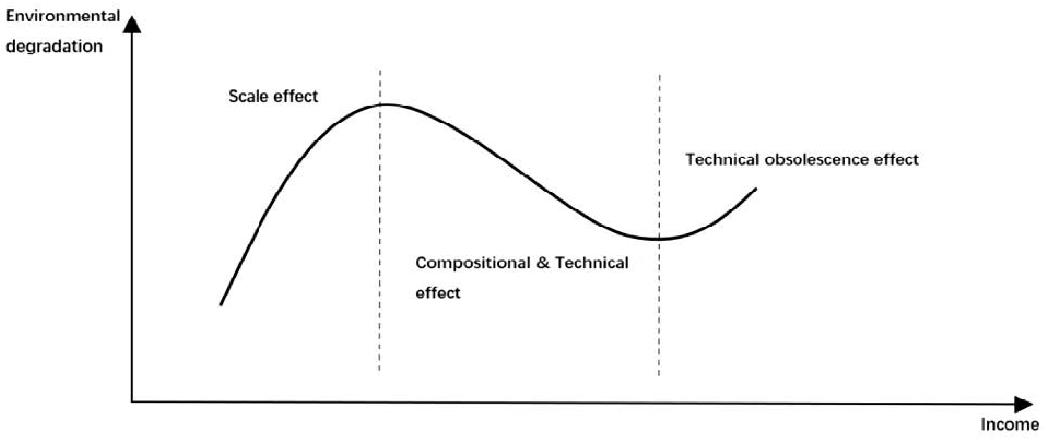
Nowadays, the inverted U-shaped EKC hypothesis has become the most debated research topic for both environmental economists and young researchers (Kasioumi and Stengos 2020; Kalaitzidakis et al. 2018; Soberon and D’Hers 2020; Kang et al. 2016; Aruga 2017, 2019). In an article, Lorente and Álvarez-Herranz (2016) further explored the topic and introduced the N-shaped hypothesis, including the third stage, where environmental degradation exacerbates as income continues to grow. The logic behind the N-shaped EKC hypothesis is that, at the first stage, there is a scale effect when the government pays attention to the national income, production, and employment more than energy conservation and environment protection. At the second stage, there is a composition and technological effect when the policymakers shift their focus on reducing the pollution level (Vita 2008; Koilo 2019; Porrini 2016). In the third stage, there is a technological obsolescence effect that appears if innovation activities reach their limitation and the technical effect is outweighed by the scale effect; thus, leading the environment to deteriorate with income again. Figure 1 depicts the three stages of the N-shaped EKC hypothesis. Hence, identifying the relationship between energy utilization, environmental degradation, and economic development is a hot research topic.

China has become an interesting topic for EKC studies for its rapid economic growth, large demand for fossil fuel consumption, and rising environmental degradation. Recent studies have examined the inverted U-shaped EKC hypothesis for China and provided policy implication based on it (Ren et al. 2014; Li et al. 2016; Wang et al. 2016). The N-shaped EKC may lead to potential challenges for the Chinese government to accomplish its carbon emission abatement goal, which is illustrated in the Copenhagen Accord and the Paris commitments, such as peaking CO₂ emissions no later than 2030. Therefore, this study aims to investigate the existence of the N-shaped EKC hypothesis and provide fresh policy implications based on the findings. However, both the autoregressive distributed lag (ARDL) model and quantile regression are adopted. If this new hypothesis is verified for China, then the current policy decision-making should be revised, taking into account the technological obsolescence effect, to prevent CO₂ emissions from rising again in the future.

In terms of methodology and variables, to the best of my knowledge, this paper is the first that adopts both the ARDL model and quantile regression to test the validity of the N-shaped EKC hypothesis in China, including energy consumption, trade openness, and urbanization simultaneously. The results have policy implications, as it is crucial for the Chinese government to ascertain the stage for effective decision-making. If there exists an N-shaped relationship between income and environmental degradation, then the EKC hypothesis should contain three stages instead of the initial two. Therefore, further measures by policymakers should take into consideration the technological obsolescence effect, to successfully peak China’s CO₂ emission by 2030 without it rising again in the future.

The article is organized as follows: in Section 2, the theoretical background with related work is discussed. Section 3 contains an explanation of the data and the methodology used in the research. Section 4 provides the results and analysis. Finally, Section 5 gives the conclusions and suggestions that are drawn for the future.

2. Theoretical Background

For decades, the literature has formed a consensus to lay a focus on major environmental pollutants, such as GHG, SO₂, and wastewater as representatives of environmental degradation to study the EKC hypothesis. Among them, GHG emissions are regarded as the principal causes of global warming that are threatening our environment as well as human society. The most intensively studied pollutant is CO₂, which accounts for 76% of the total GHG emissions, according to the Center for Climate and Energy Solutions. To address the omitted variable biases, researchers have been employing a multivariate framework and incorporating several independent variables other than income. These factors not only contribute to understanding the causal effect of CO₂ emissions and other pollutants, but also help to re-examine the validity of the EKC hypothesis. Some of the introduced variables include foreign direct investment (Ali et al. 2017; Abdouli et al. 2018), trade openness (Pata 2018; Destek et al. 2018), energy consumption (Pablo-Romero and De Jesús 2016; Pal and KumarMitra 2017), urbanization, corruption (Leitão 2010; Masron and Subramaniam 2018; Quéré et al. 2018), and technology and energy innovation (Jiang et al. 2019; He and Jiang 2012; Bölük and Mert 2015; Saudi et al. 2019). Following (Li et al. 2016), this study selects the combination of variables of energy consumption, urbanization, and trade openness, to test the EKC hypothesis in China. Each variable has its important economic implication that is relevant to CO₂ emissions.

Energy consumption is the most frequently adopted determinant in the study of the EKC hypothesis, which contains both renewable energy and fossil fuel consumption. Many papers have founds a significantly positive effect of energy consumption on CO₂ emissions (Baek and Gweisah 2013; Saudi et al. 2019). The inclusion of trade openness and urbanization are comparatively less obvious than energy consumption, though they are both regarded as important factors of CO₂ emission. Three major schools of thought explain the mixed effects of trade openness on CO₂ emissions. First, trade openness provides access to international markets for each country, thus leading to more competition, which encourages international companies and local governments to enhance energy innovation and the efficiency of using energy as a cause of decreasing CO₂ emissions (Shahbaz et al. 2012). Second, the expansion of production due to trade openness increases CO₂ emissions (Lopez and Islam 2008). Third, the shifting of heavily polluting industries to the developing world and the pollution haven hypothesis contributes to an increase of CO₂ emissions in developing countries and a reduction in developed countries (Grossman and Krueger 1991). As a result, the effect of trade openness is multiple and, thus, has different aggregate effects. Articles (Jalil and Feridun 2011) and (Li et al. 2016) found a negative relationship between trade openness and CO₂ emission in China, while (Jayanthakumaran et al. 2012) considered such effect insignificant. However, an article (Wang et al. 2011) estimated that a 1% increase in per capita energy consumption would lead to a 4.7% increase in carbon emissions.

The effects that urbanization has on environmental quality also have two directions. First, there is a negative effect, as urban areas tend to have intense industrial concentration and congestion. Second, there is a positive effect on the environment due to abatement policies and technology innovations that are easier to conduct in areas of higher population density (Farzin and Bond 2006; Wang et al. 2016). Such mixed effects are confirmed by the literature. Article (Li et al. 2016) confirmed a significantly positive long run effect of urbanization on CO₂ emissions in China, while (Qu and Zhang 2011) deemed these effects insignificant.

Since the 1990s, many studies have discussed the validity of the EKC hypothesis and explored the existence of an inverted U-shaped relation between income and environmental degradation. However, there is no consensus in the literature about the hypothesis in China. For example, using panel data analysis for both SO₂ and CO₂ emissions, (Yaguchi et al. 2007) compared situations in Japan and China, and demonstrated that the EKC hypothesis is supported in the case of Japan but does not exist in the case of China. The panel cointegration estimation conducted by (Wang et al. 2011) failed to confirm the EKC hypothesis, after examining CO₂ emissions and income in China. However, (Wang et al. 2016) employed panel data approaches and semi-parametric panel fixed effects regression from 1990 to 2012 and confirmed the validity of the EKC hypothesis for SO₂. Article (Li et al. 2016) used an ARDL model together with the General Method of Movement (GMM) approach and found an inverted U-shaped feature for CO₂ emissions, wastewater emissions, and waste solid emissions. Moreover, (Pal and KumarMitra 2017) conducted a comparative study between India and China, using an ARDL model of time series data, and concluded the N-shaped relationship between CO₂ emission per capita and GDP per capita.

Due to the Coronavirus Disease (COVID-19) lockdown, carbon emissions in China will be reduced dramatically. According to the Centre for Research on Energy and Clean Air, it is not expected to have a long-term impact. Similarly, in India, after the first lockdown for COVID-19 in March 2020, energy consumption reduced dramatically. However, upon the relaxation of lockdown, energy consumption started to increase again (Aruga et al. 2020). A summary of the selective studies of recent years is presented in

Table 1. Summary of the selective relevant studies.

Author (s)	Country/Countries	Period	Methodology	Major Variables	Results
Shahbaz et al. (2018)	France	1955–2016	ARDL	GDP per capita, FDI, Financial development	Inverted U-shape association between CO2 and GDP
Apergis et al. (2017)	United States	1960–2010	Common Correlated Effects	GDP per capita, GM-FMOLS, GM-DOLS	Inverted U-shape association between CO2 and personal income
Alam and Adil (2019)	India	1971–2016	ARDL	GDP per capita, CAAGR	insignificant relationship between CO2 and GDP
Rafindadi (2016)	Japan	1971–2012	ARDL	GDP per capita, Fukushima energy crisis	Inverted U-shape association between CO2 and GDP
Pal and KumarMitra (2017)	China and India	1971–2012	ARDL	Per capita GDP, AIC, SBC	N-shape association between CO2 and GDP
Shahbaz et al. (2017)	China	1970–2012	ARDL	GDP per capita, VECM, ECM	Inverted U-shape relationship between CO2 and GDP
Li et al. (2016)	China	1996–2012	ARDL and GMM	GDP, DFE, PMG	Inverted U-shape relationship between CO2 and GDP
Wang et al. (2016)	China	1990–2012	Panel Fixed Effects Regression	GDP per capita, Economic growth, STIRPAT	Inverted U-shape association between SO2 and GDP
Ren et al. (2014)	China	2000–2010	GMM	GDP, EEE, EEI, EEB, FDI	Inverted U-shape relationship between CO2 and GDP

Source: own elaboration. Note: Foreign Direct Investment (FDI), Group Mean Fully Modified OLS (GM-FMOLS), Group Mean Dynamic OLS (GM-DOLS), Compound Average Annual Growth Rate (CAAGR), Akaike Information Criteria (AIC), Bayesian Information Criteria (SBC), Vector error correction method (VECM), Error Correction Model (ECM), Dynamic Fixed Effects (DFE), Pooled Mean Group (PMG), Stochastic Impacts by Regression on Population Affluence and Technology (STIRPAT), Sulfur Dioxide (SO₂), Emissions Embodied in Exports (EEE), Emissions Embodied in Imports (EEI) and, Emissions Embodied in Trade (EEB).

.

Table 1 represents the relevant literature in several aspects. The literature and policymakers have focused on the emission-growth nexus under the inverted U-shaped EKC hypothesis.

3. Data and Methodology

3.1. Data

To carry out empirical analysis, the annual time series dataset from 1971 to 2014 is constructed from two sources: China Statistical Yearbook and the World Development Indicators (WDI). To measure environmental pollution, yearly CO₂ per capita in metric tons is extracted from WDI, which is calculated by the Carbon Dioxide Information Analysis Center (CDIAC). Annual real GDP per capita (constant 2010 US$) from WDI is used for the estimation as a proxy for income. The annual energy consumption per capita in kilograms of oil equivalent is available up to 2014 from WDI. The share of total imports and exports (% of GDP) is used to represent trade openness. As a proxy for the level of urbanization, the proportion of the urban population in China is extracted from the China Statistical Yearbook. All variables are in the form of a natural logarithm.

3.2. Methodology

To execute the effective analysis ARDL modeling approach has been used in this study. Moreover, the bounds test is adopted for cointegration to estimate the long run relationship between CO₂ emissions and other variables. These approaches were developed by (Pesaran et al. 1999, 2001). Unlike the Vector Autoregression (VAR) model that is strictly employed for endogenous variables, ARDL specification uses both endogenous and exogenous variables. ARDL has advantages in the study of the growth environment nexus for several reasons. First, compared with other cointegration tests, the Johansen approach is less favorable than the ARDL model for small and finite sample sizes, which is a common feature in EKC analysis within China. Second, though the ARDL model requires that no variables are integrated of order 2, it can be applied whether these variables are integrated of order 1, integrated of order 0, or have a combination of I(1) and I(0) order of integration. Third, the ARDL model is involved in only one equation setting, which makes it simpler to estimate and interpret than other techniques that require multiple equations to be set-up. Finally, the ARDL model simultaneously generates short-run relationships by the ECM and the long run coefficients.

The basic theoretical model for CO₂ emission is $lnco2=f\left(lny, ln{y}^2, ln{y}^3, lnec, lnto, lnu\right)$. The cubic parametric model specification is constructed as follows to test the N-shaped hypothesis:

$$lnco{2}_t={\beta }_0+{\beta }_{1}ln{y}_t+{\beta }_{2}ln{y}_t^2+{\beta }_{3}ln{y}_t^3+{\beta }_{4}lne{c}_t+{\beta }_{5}lnt{o}_t+{\beta }_{6}ln{u}_t+u_t$$

(1)

In Equation (1), $lnco{2}_t$ is the logarithmic transformation of CO₂ emissions per capita, $ln{y}_t$ is the natural logarithm of real GDP per capita, $ln{y}_t^2$ and $ln{y}_t^3$ are the squared and cubic terms for real GDP per capita. $lne{c}_t$represents the logarithmic transformation of energy consumption per capita. $lnt{o}_t$denotes the natural logarithm of total import and export share in GDP. $ln{u}_t$is the natural logarithm of the proportion of the urban population. Finally, $u_t$ is the random error ($t=$ time period $=1, 2, \dots , n$). In this study, according to the N-shaped hypothesis, ${\beta }_1>0$, ${\beta }_2<0$, ${\beta }_3>0$ needs to be justified. If ${\beta }_1>0$, ${\beta }_2<0$ and ${\beta }_3$ is insignificant, then the conventional EKC is confirmed while the N-shaped hypothesis fails to be supported. If both ${\beta }_1$ and ${\beta }_2$ are insignificant, then the validity of EKC cannot be confirmed in China. Meanwhile, ${\beta }_4$ is expected to be positive as more energy consumption generates more CO₂ emissions. However, the signs of ${\beta }_5$ and ${\beta }_6$ are unclear due to their mixed effects on the environment. Each of them can be either positive or negative.

The estimation of the ARDL model follows several processes. Firstly, the bounds test is utilized to determine the cointegration among the variables. Articles (Pesaran et al. 2001) provided critical values for testing the null or empty hypothesis of no cointegration. For I(1) time series, under a certain significant level, if the output F-statistics is larger compared to the upper bound critical value, then we fail to reject the null or empty hypothesis, and it is concluded that there is a long-running relationship within the variables. Next, the ARDL equation to the estimation is constructed as below,

$$lnco{2}_t={\alpha }_0+{\sum }_{i=1}^p{\delta }_{i}lnco{2}_{t-i}+{\sum }_{j=1}^6{\sum }_{i=0}^{q_j}{\phi }_{ij}{V}_{jt-i}+{\epsilon }_t$$

(2)

In Equation (2), $V_t$ is the vector of all independent variables, ${\epsilon }_t$represents the error term, and the maximum of lags, $p$ and $q_j$ are determined frequently by the Akaike Information Criteria (AIC), the final prediction error (FPE), and the Schwartz Information Criteria to determine the optimal ARDL specification. This study selects the AIC to calculate the optimal lag values since the AIC is a more advantageous understudy in the case of a small sample, which is less than 60 observations (Liew 2004). In the case of cointegration, the last step in the ARDL procedure is to estimate the short-run coefficients according to the ECM, specified as,

$$\mathsf{\Delta }lnco{2}_t={\lambda }_0+{\sum }_{i=1}^p{\psi }_i\mathsf{\Delta }lnco{2}_{t-i}+{\sum }_{j=1}^6{\sum }_{i=0}^{q_j}{\omega }_j\mathsf{\Delta }{V}_{jt-i}+\theta EC{T}_{t-1}+e_t$$

(3)

In Equation (3), ${\psi }_i$ and ${\omega }_j$ are denoted as short-term coefficients, $\theta$ represents the speed of tuning parameter, the error correction part $EC{T}_{t-1}$ is the residual series from the results of the estimated cointegration model. The sign of the speed of adjustment parameter must be negative, ranging from $-1$ to $0$, to support the long run convergence within the variables. It also indicates that previous errors will be corrected in the current period.

The Augmented Dickey–Fuller (ADF) and Phillips–Perron (PP) tests are employed to test for unit root before the ARDL approach. Furthermore, the quantile regression as a robust inference approach is used to validate the results in ARDL estimation. The quantile regression helps to explore the full spectrum of the conditional quantiles for evaluating the contemporaneous relationship between excess returns and expected risk. Particularly, instead of modeling “mean” the excess results using a least squares approach, a quantile regression approach measures the quantiles of the conditional order of the excess returns, which are represented as functions of observed covariates. The coefficients in the quantile regression equation are functions with a dependency on the quantile and are estimated by reducing the median absolute deviation determined by the loss function ${\rho }_{\tau }\left(u\right)=u\left(\tau -1_{\left\{u<0\right\}}\right)$. One advantage of the quantile regression introduced by (Koenker and Bassett 1978), is that it takes into consideration the conditional distribution of the variables that cannot be explained by the Ordinary Least Squares (OLS) regression. Finally, some diagnostic tests are adopted, including tests for serial correlation, heteroscedasticity, and structural stability to ascertain how well the model fits.

4. Results and Analysis

4.1. Unit Root Test

Table 2. Descriptive statistics.

	Mean	Std. Dev.	Min	Max	Skewness	Kurtosis
$lnco2$	0.93	0.59	0.04	2.02	0.43	2.18
$lny$	6.92	1.04	5.47	8.72	0.17	1.75
$ln{y}^2$	48.95	14.56	29.97	75.96	0.33	1.85
$ln{y}^3$	353.50	155.88	164.03	662.02	0.49	2.00
$lnec$	9.23	0.47	8.60	10.17	0.70	2.35
$lnto$	3.23	0.70	1.59	4.17	−0.65	2.37
$lnu$	3.37	0.38	2.84	4.00	0.13	1.74

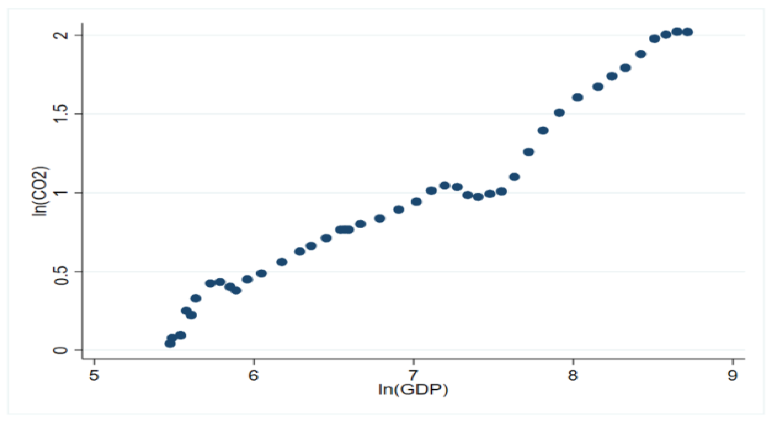
Source: author’s calculation. Note: $lnco2, lny, ln{y}^2, ln{y}^3,lnec, lnto, and lnu$ indicate the logarithmic transformation of CO₂ emissions, natural logarithm, the squared term, the cubic term, the logarithmic transformation of energy consumption, the natural logarithm of total import and export share in GDP, and the logarithm of the proportion of the urban population, respectively.

delineates the descriptive statistics data of the variables and Figure 2 depicts the relationship between carbon emission and economic growth in the scatter plot. Before the bounds test, a unit root test for the concerned variables is necessary to ensure that none of the variables is integrated of order more than unity. This study used the ADF and PP approaches to test for stationarity of the underlying variables.

Table 3. Unit root tests output.

	ADF Test		PP Test
	Level Form
Variables	Intercept	Trend and Intercept	Intercept	Trend and Intercept
$lnco2$	0.891	−1.031	0.473	−1.566
$lny$	2.750	−3.880	2.078	−3.652 **
$ln{y}^2$	5.056	−2.934	3.755	−2.650 **
$ln{y}^3$	7.612	−1.784	5.514	−1.594
$lnec$	2.031	−0.435	1.339	−0.877
$lnto$	−2.924 ***	−1.688	−2.894 **	−1.789
$lnu$	1.772	−3.795	1.049	−3.419 **
	First difference
$Dlnco2$	−3.448 ***	−3.414 **	−3.521 ***	−3.495 **
$Dlny$	−4.117 ***	−4.342 ***	−4.071 ***	−4.318 ***
$Dln{y}^2$	−3.229 ***	−4.042 ***	−3.133 **	−4.014 ***
$Dln{y}^3$	−2.447 ***	−3.776 **	−2.313	−3.760 **
$Dlnec$	−3.565 ***	−3.742 **	−3.621 ***	−3.811 **
$Dlnto$	−4.849 ***	−5.282 ***	−4.726 ***	−5.181 ***
$Dlnu$	−3.936 ***	−3.809 **	−3.908 ***	−3.803 **

Source: author’s calculation. Note: $**$and $***$ indicate $5\%$ and $1\%$ of significant levels, respectively. $D$ represents the first difference operator.

highlighted the outputs of the unit root test. The unit root test results indicate that, although the underlying variables are non-stationary at level value, they are stationary at the first difference, which provides the prerequisite for using the ARDL approach.

4.2. The Bounds Test

The F-statistics reported from the bounds test are highly sensitive to the chosen lag lengths when testing the cointegration among variables. In this study, AIC is adopted to reach the optimal lag length for each variable, since AIC lag specification works better than the others in the small sample time series. The AIC suggests that the bounds test results and the optimum lag length is equal to (2, 2, 1, 2, 2, 2, 1) for ($lnco2,lny,ln{y}^2, ln{y}^3, lnec, lnto, lnu$).

Table 4. Autoregressive distributed lag (ARDL) bounds test results.

			I(0)	I(1)
Model	$lnco2=f\left(lny, ln{y}^2, ln{y}^3, lnec, lnto, lnu\right)$
	Without Deterministic Trends
K = 6	$F_{iii}$	3.472 *	2.12	3.23
	With Deterministic Trends
K = 6	$F_v$	4.693 **	3.19	4.38

Source: author’s calculation. Notes: $k$ represents the number of independent variables.$*$ and $**$ indicate $10\%$ and $5\%$ of significant levels, respectively.

indicates that, with the present CO₂ emission equation ($lnco2=f\left(lny, ln{y}^2, ln{y}^3, lnec, lnto, lnu\right)$), the F-statistics (Case 3, = 3.472) exceeds the higher limit values at 10% significant level without deterministic trends, and the F-statistics (Case 5, = 4.693) exceeds the higher limit critical values at the 5% level of significance with deterministic trends. This resulted in the rejection of the null hypothesis that no cointegration exists and tends to be in favor of the alternative. Apart from the findings by Jayanthakumaran et al. (2012) that indicated inconclusive F-statistics for China when setting per capita CO₂ emission as dependent variables, the bounds test result in this paper highlights cointegration and the long run movement between CO₂ emissions, real GDP along with its squared and cubic terms, urbanization, energy consumption, and trade openness. Moreover, the estimation agrees with the findings by Pal and KumarMitra (2017) that compared the econometric model in China with that in India.

4.3. Short-Term and Long-Term Analysis

Table 5. Estimation of Error Correction Model (ECM) and ARDL level equation.

	With Constant			With Constant and Trend
Variable	Coefficient	Std. Error	t-Statistic	Coefficient	Std. Error	t-Statistic
Long run coefficients
$lny$	8.34	2.66	3.13 ***	6.62	1.61	4.12 ***
$ln{y}^2$	−1.14	0.38	−3.02 ***	−0.84	0.23	−3.63 ***
$ln{y}^3$	0.05	0.02	2.93 ***	0.04	0.01	3.33 ***
$lnec$	0.90	0.19	4.69 ***	1.19	0.14	8.68 ***
$lnto$	0.03	0.09	0.36	0.00	0.05	0.10
$lnu$	−0.34	0.24	−1.40	−0.26	0.15	−1.74 *
Short-run coefficients
$Dlny$	−7.77	12.67	−0.61	−20.63	13.02	−1.59
$Dln{y}^2$	1.16	1.89	0.61	3.04	1.93	1.57
$Dln{y}^3$	−0.06	0.09	−0.60	−0.15	0.09	−1.56
$Dlnec$	0.14	0.27	0.52	−0.34	0.33	−1.01
$Dlnto$	0.00	0.04	−0.12	−0.02	0.03	−0.46
$Dlnu$	0.09	0.33	0.27	0.26	0.31	0.84
Constant	−20.23	6.75	−3.00 ***	−0.02	0.01	−2.25 **
$ECT\left(-1\right)$	−0.75	0.22	−3.43 ***	−1.18	0.28	−4.25 ***
$R^2$		0.91			0.93
$Adj R^2$		0.84			0.87
RMSE		0.02			0.02
Log-likelihood		120.30			124.64

Source: author’s calculation. Notes: $ECT\left(-1\right)$ represents the error correction term or the adjustment parameter. The Root Mean Square Error (RMSE) is considered as a measurement of residual and thus model accuracy. The model is more accurate if $RMSE$ is closer to zero. The symbol $*$, $**$, and $***$ indicate $10\%$, $5\%,$ and $1\%$ of significant levels, respectively.

delineated both short-term and long-term coefficients for the model specification. The error correction terms are significant and have expected negative signs. In accordance with the hypothesis of this study, the long run coefficient for real GDP along with its squared and cubic forms are, $8.34$,$-1.14,$ and $0.05$, respectively, with only the constant, $6.62$, $-0.84,$ and $0.04$, respectively, with the constant and trend. The Error correction term $ECT\left(-1\right)$ is equal to $-0.75$ in the model with constant, which means that CO₂ emissions touch the equilibrium by 75% speed of tuning in the long-term, affected by income, energy consumption, trade openness, and urbanization.

As specified in Equation (3), the long run outputs in the table indicate that all of the elasticities of the respective variables are as expected and are statistically significant. At the first stage, CO₂ emissions rise with income and after reaching a certain threshold value at the second stage, CO₂ emissions decrease with income. Finally, in the third stage, CO₂ emissions rise again with the economy. These results support that the N-shaped curve for CO₂ emissions exists in the long run. A technological obsolescence effect exists that drives the path of environmental degradation up again into the third stage. In accordance with the literature, such as Wang et al. (2011), the estimated elasticity for energy consumption indicates a directly negative effect of output on environmental quality in China in the long run. It suggests that an increase in per capita energy consumption, by 1%, will result in an increase in carbon emissions by 4.7%. Unlike the finding by Li et al. (2016), the negative long-term elasticity of urbanization on environmental degradation implies that the composition effect exceeds the scale effect through the development of urbanization in China. This means that the positive effect in urban areas, due to abatement policies and technology innovation, outweighs the negative effect due to intense industrial concentration and congestion.

From Table 5, it is estimated that if energy consumption rises by $1\%$, CO₂ emissions will correspondently rise by $0.9\%$ in the long run, though the elasticity of trade openness is not substantial. If urbanization under the model with constant and trend is positively significant at the 10% level, which expresses that the theoretically mixed effect of urbanization on environmental quality tends to be positive in China, this means that the development of urbanization in China is leading to less environmental degradation. On the contrary, the short-run elasticities do not provide evidence for the N-shaped curve for CO₂ emissions specified in Equation (1) in the short term, suggesting that the N-shaped pattern only exists in the long-term.

Since the OLS approaches have been criticized for restricting the estimators to be unchanged across all percentiles, the quantile regression is adopted as a robust inference test.

The results of quantile regression are presented in

Table 6. Quantile regression results.

Variable	Percentile
	10	20	30	40	50
$lny$	2.4864 ***	3.4575 ***	3.7372 **	3.646 **	3.8602 ***
$ln{y}^2$	−0.2514 **	−0.413 **	−0.45 **	−0.4391 **	−0.452 ***
$ln{y}^3$	0.0092	0.0171 *	0.0187 *	0.0183 *	0.0177 **
$lnec$	1.1746 ***	1.1727 ***	1.1559 ***	1.1611 ***	1.2145 ***
$lnto$	0.0102	0.0621	0.0344	0.0306	−0.0337
$lnu$	−0.7744 ***	−0.5804 ***	−0.4952 **	−0.4971 **	−0.3168 **
Constant	−15.5107 ***	−17.9291 ***	−18.6407 ***	−18.4156 ***	−19.9425 ***
Pseudo $R^2$	0.9615	0.9597	0.9628	0.9636	0.9649
	60	70	80	90
$lny$	4.3544 ***	4.3266 ***	4.3186 ***	2.2999 ***
$ln{y}^2$	−0.5183 ***	−0.5113 ***	−0.5129 ***	−0.2206 **
$ln{y}^3$	0.0205 ***	0.02 ***	0.0202 ***	0.006
$lnec$	1.2483 ***	1.2728 ***	1.2606 ***	1.3333 ***
$lnto$	−0.0536 *	−0.0558 **	−0.0495 **	−0.0374 *
$lnu$	−0.2738 *	−0.2983 **	−0.3139 ***	−0.2772 ***
Constant	−21.4865 ***	−21.6034 ***	−21.411 ***	−17.5325 ***
Pseudo $R^2$	0.9685	0.973	0.9751	0.9756

Source: author’s calculation. Notes: $*$, $**$ and $***$ indicate $10\%$, $5\%,$ and $1\%$ of significant levels, respectively.

. In accordance with the results from the ARDL model, the level and quadratic form of actual GDP per capita are significant and have predictable signs in all percentiles. The cubic form of actual GDP per capita is significantly positive in all quantiles except the 10th and 90th, which are smaller compared to the results these found from the ARDL model. Due to this reason, the 10th and 90th quantiles demonstrate an inverted U-shaped EKC. In other words, the N-shaped association between CO₂ and GDP is confirmed in quantiles from the 20th to 80th, while in the 10th and 90th quantiles, an inverted U-shaped EKC is found instead of the N-shaped one. The coefficients of power consumption and urbanization are significantly positive and negative, respectively, in all quantiles, which correlates to the outputs from the ARDL model.

Table 7. Diagnostic test results.

Test	Statistics		Probability
Durbin–Watson	D-statistic	2.11
Breusch–Godfrey LM	chi2	11.27	0.0036
Breusch Pagan	chi2	0.00	0.9576
White’s	chi2	42.00	0.4274
Ramsey RESET	F-statistics	1.49	0.2473

Source: author’s calculation.

depicts the outputs of the diagnostic tests. According to the Durbin–Watson approach and Breusch–Godfrey Lagrange Multiplier (LM) test, the econometric model for $lnco2$does not suffer from slightly negative autocorrelation. The $chi2$ statistics of the Breusch–Pagan test and White’s test indicate that the model is free from the problem of heteroscedasticity. The result of the Ramsey Regression Equation Specification Error Test (RESET) suggests that the nonlinear combinations of real GDP help in describing the dependent variable.

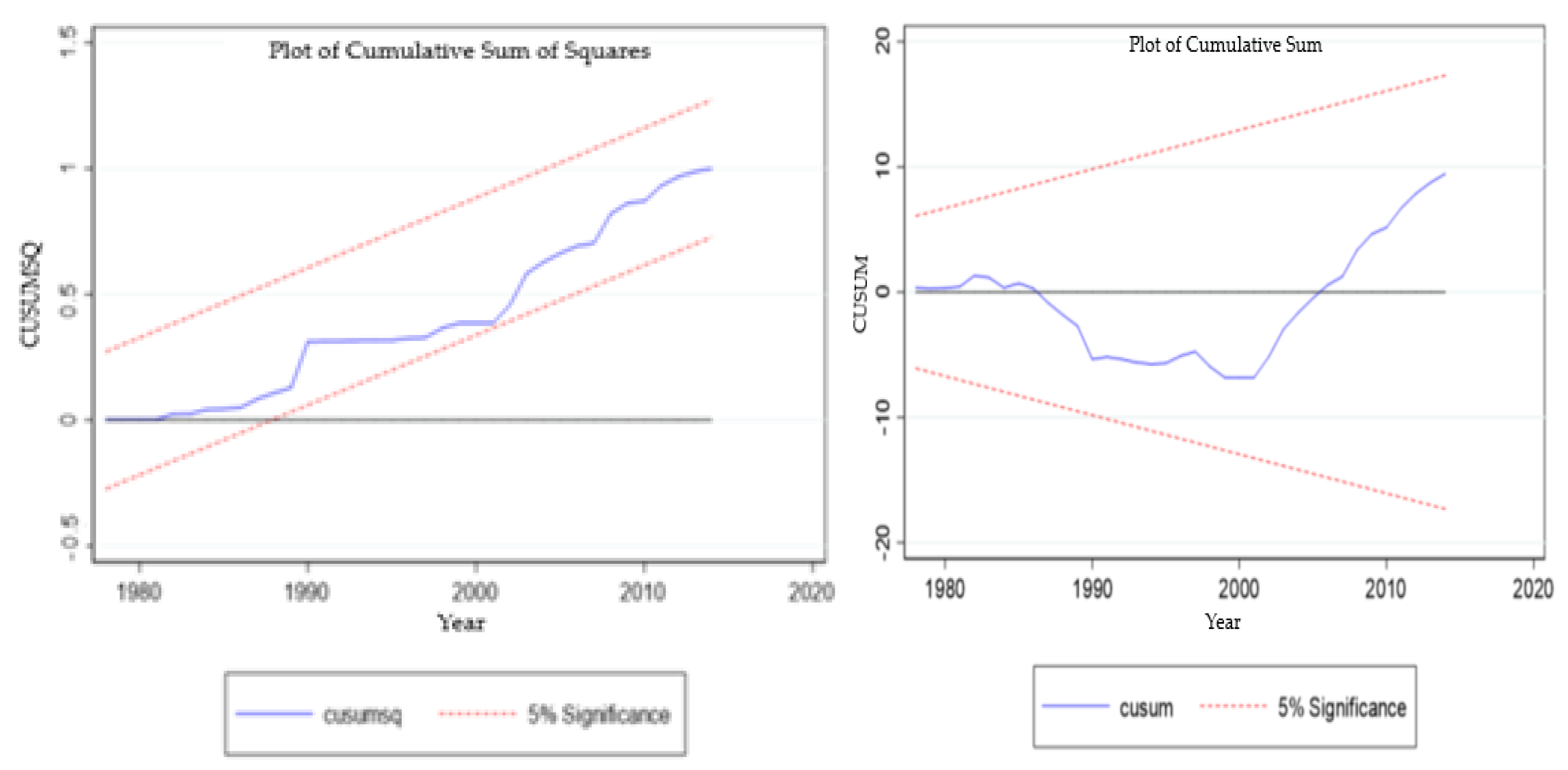
Figure 3 depicts the plots of the Cumulative Sum of Squares (CUSUMSQ) and the Cumulative Sum (CUSUM) tests for the ARDL estimation, which are regarded as approaches to checking stability in the estimators. The blue line indicates the cumulative sum of deviations. The black line is the centerline located at zero. The dashed lines are the control limits that are located four standard deviations from the centerline. The plots are well-around $95\%$ critical bounds, and it can be inferred that all estimators in the ARDL specification are stable over the period from 1971 to 2014, and will not be significantly distorted by policy implementation.

5. Conclusions and Policy Implications

This study analyzes the CO₂ growth nexus while controlling energy consumption, trade openness, and urbanization simultaneously, using available time-series data. Based on the findings in this study, the EKC hypothesis is verified for China in the long run. Moreover, though the estimated contemporaneous association between carbon emissions and the economy in Table 5 do not provide significant evidence in the short run, the N-shaped relationship, in the long run, has been validated. Apart from the comforting findings in the literature that support the conventional U-shaped EKC hypothesis, the N-shaped relationship between environmental degradation and income found in this paper appears to be more precarious as the environment quality is likely to deteriorate further in the long run. The coefficients estimated in this study indicate that economic growth, globalization, trade liberalization, and energy consumption can pose potential problems for the environment quality and, thus, derail the goals of the Chinese government as promised in the Paris Agreement. Even if China is capable of peaking its CO₂ emissions by 2030, there is still uncertainty that CO₂ emissions may rise again with national income further into the future.

In 2018, the Chinese government launched a policy that requires 480 million tons of carbon capacity from steel production to meet the low-carbon standards by 2020. Although, according to the 13th Five-Year Plan (FYP), China has achieved 15% share of renewable energy consumption in 2020, the country sees continued expansions of fossil infrastructure in recent years. Despite the reduction of carbon emissions in China caused by COVID-19, the Centre for Research on Energy and Clean Air declared that it is not expected to have a long-term impact. In 2020, President Xi has announced that the country aims to peakCO₂ emissions by 2030 and achieve carbon neutrality by 2060. Therefore, in an attempt to avoid the technological obsolescence effect moving towards the third stage, a breakthrough, in terms of policy decision-making and energy innovation, is required for the 14th FYP to begin in 2021.

China, still the largest carbon emitter, needs to reform its abatement and energy policies to prevent the environment from deteriorating again after the apex. The energy consumption in China is expected to increase rapidly as the economy and globalization in China continue to rise. Energy and technology innovation plays an essential part in reducing GHG emissions, particularly in urban areas. However, the results of this paper indicate that technological innovation may not be enough to prevent the environment from deteriorating again. Both market-based pricing instruments and command and control regulations are indispensable under China’s specific socioeconomic and political circumstances. Moreover, the development of renewable energy, national and provincial laws, fiscal policies, and other regulations, need to be adopted to reinforce the efficiency of energy use. Inefficient coal-fired power plants should be phased out. Citizens are encouraged to use public transportation and new energy (electric) vehicles. Producers are motivated to introduce new methods of production and organization to lower carbon emissions. Furthermore, export product structure and the composition of foreign investment are required to become more environmentally friendly. Low carbon industries and high-quality investments are looked on more favorably for entering China’s market.

This paper provides new evidence for the current policy of decision-making to enhance the understanding of the growth-pollution nexus. However, further research is required to investigate the role of energy and technological development, including the relationship between environmental degradation and trade openness in China.

References

- Abdouli, Mohamed, Olfa Kamoun, and Besma Hamdi. 2018. The Impact of Economic Growth, Population Density, and FDI Inflows on CO2 Emissions in BRICTS Countries: Does the Kuznets Curve Exist? Empirical Economics 54: 1717–42. [Google Scholar] [CrossRef]
- Abeydeera, Lebunu, Hewage Udara Willhelm, Jayantha Wadu Mesthrige, and Tharushi Imalka Samarasinghalage. 2019. Global Research on Carbon Emissions: A Scientometric Review. Sustainability (Switzerland) 11: 3972. [Google Scholar] [CrossRef] [Green Version]
- Aguila, Yann. 2020. A Global Pact for the Environment: The Logical Outcome of 50 Years of International Environmental Law. Sustainability (Switzerland) 12: 5636. [Google Scholar] [CrossRef]
- Alam, Riyaz, and Masudul Hasan Adil. 2019. Validating the Environmental Kuznets Curve in India: ARDL Bounds Testing Framework. OPEC Energy Review 43: 277–300. [Google Scholar] [CrossRef]
- Ali, Wajahat, Azrai Abdullah, and Muhammad Azam. 2017. Re-Visiting the Environmental Kuznets Curve Hypothesis for Malaysia: Fresh Evidence from ARDL Bounds Testing Approach. Renewable and Sustainable Energy Reviews 77: 990–1000. [Google Scholar] [CrossRef]
- Apergis, Nicholas, Christina Christou, and Rangan Gupta. 2017. Are There Environmental Kuznets Curves for US State-Level CO2 Emissions? Renewable and Sustainable Energy Reviews 69: 551–58. [Google Scholar] [CrossRef] [Green Version]
- Aruga, Kentaka, Md Monirul Islam, and Arifa Jannat. 2020. Effects of COVID-19 on Indian Energy Consumption. Sustainability (Switzerland) 12: 5616. [Google Scholar] [CrossRef]
- Aruga, Kentaka. 2017. Does the Energy-Environmental Kuznets Curve Hypothesis Sustain in the Asia-Pacific Region? Munich Personal RePec Archive no. 80692. Munich: University Library of Munich, Germany, pp. 1–15. [Google Scholar]
- Aruga, Kentaka. 2019. Investigating the Energy-Environmental Kuznets Curve Hypothesis for the Asia-Pacific Region. Sustainability (Switzerland) 11: 2395. [Google Scholar] [CrossRef] [Green Version]
- Baek, Jungho, and Guankerwon Gweisah. 2013. Does Income Inequality Harm the Environment?: Empirical Evidence from the United States. Energy Policy 62: 1434–37. [Google Scholar] [CrossRef]
- Bölük, Gülden, and Mehmet Mert. 2015. The Renewable Energy, Growth and Environmental Kuznets Curve in Turkey: An ARDL Approach. Renewable and Sustainable Energy Reviews 52: 587–95. [Google Scholar]
- Boumphrey, Sarah. 2014. China Overtakes the US as the World’s Largest Economy: Impact on Industries and Consumers Worldwide. Euro Monitor International. Available online: https://www.iimk.ac.in/libportal/reports/China-Overtakes-US-Worlds-Largest-Economy-White-Paper-Euromonitor-Report.pdf (accessed on 20 December 2020).
- Brandt, Loren, Debin Ma, and Thomas G. Rawski. 2014. From divergence to convergence: Reevaluating the history behind China’s economic boom. Journal of Economic Literature 52: 45–123. [Google Scholar] [CrossRef] [Green Version]
- Destek, Mehmet Akif, Recep Ulucak, and Eyup Dogan. 2018. Analyzing the Environmental Kuznets Curve for the EU Countries: The Role of Ecological Footprint. Environmental Science and Pollution Research 25: 29387–96. [Google Scholar] [CrossRef]
- Farzin, Y. Hossein, and Craig A. Bond. 2006. Democracy and Environmental Quality. Journal of Development Economics 81: 213–35. [Google Scholar] [CrossRef]
- Grossman, Gene, and Alan B. Krueger. 1991. Environmental Impacts of a North American Free Trade Agreement. Cambridge: National Bureau of Economic Research. [Google Scholar]
- Grossman, Gene, and Alan B. Krueger. 1995. Economic Growth and the Environment. The Quarterly Journal of Economics 110: 353–77. [Google Scholar] [CrossRef] [Green Version]
- Hanaki, Keisuke, and Joana Portugal-Pereira. 2018. The Effect of Biofuel Production on Greenhouse Gas Emission Reductions BT—Biofuels and Sustainability: Holistic Perspectives for Policy-Making. Edited by Kazuhiko Takeuchi, Hideaki Shiroyama, Osamu Saito and Masahiro Matsuura. Tokyo: Springer Japan, pp. 53–71. [Google Scholar] [CrossRef]
- He, Yu Wei, and Jin Rong Jiang. 2012. Technology Innovation Based on Environmental Kuznets Curve Hypothesis. Advanced Materials Research 573: 813–35. [Google Scholar] [CrossRef]
- Holtz-Eakin, Douglas, and Thomas M. Selden. 1995. Stoking the Fires? CO2 Emissions and Economic Growth. Journal of Public Economics 57: 85–101. [Google Scholar] [CrossRef] [Green Version]
- Jalil, Abdul, and Mete Feridun. 2011. The Impact of Growth, Energy and Financial Development on the Environment in China: A Cointegration Analysis. Energy Economics 33: 284–91. [Google Scholar] [CrossRef]
- Jayanthakumaran, Kankesu Jay, Reetu Verma, and Ying Liu. 2012. CO2 Emissions, Energy Consumption, Trade and Income: A Comparative Analysis of China and India. Energy Policy 42: 450–60. [Google Scholar] [CrossRef]
- Jiang, Lei, Shixiong He, Zhangqi Zhong, Haifeng Zhou, and Lingyun He. 2019. Revisiting Environmental Kuznets Curve for Carbon Dioxide Emissions: The Role of Trade. Structural Change and Economic Dynamics 50: 245–57. [Google Scholar] [CrossRef]
- Kalaitzidakis, Pantelis, Theofanis Mamuneas, and Thanasis Stengos. 2018. Greenhouse Emissions and Productivity Growth. Journal of Risk and Financial Management 11: 38. [Google Scholar] [CrossRef] [Green Version]
- Kang, Yan Qing, Tao Zhao, and Ya Yun Yang. 2016. Environmental Kuznets Curve for CO2 Emissions in China: A Spatial Panel Data Approach. Ecological Indicators 63: 231–39. [Google Scholar] [CrossRef]
- Kasioumi, Myrto, and Thanasis Stengos. 2020. The Environmental Kuznets Curve with Recycling: A Partially Linear Semiparametric Approach. Journal of Risk and Financial Management 13: 274. [Google Scholar] [CrossRef]
- Koenker, Roger, and Gilbert Bassett. 1978. Regression Quantiles. Econometrica: Journal of the Econometric Society 46: 33–50. [Google Scholar] [CrossRef]
- Koilo, Viktoriia. 2019. Evidence of the Environmental Kuznets Curve: Unleashing the Opportunity of Industry 4.0 in Emerging Economies. Journal of Risk and Financial Management 12: 122. [Google Scholar] [CrossRef] [Green Version]
- Leitao, Alexandra. 2010. Corruption and the Environmental Kuznets Curve: Empirical Evidence for Sulfur. Ecological Economics 69: 2191–201. [Google Scholar] [CrossRef]
- Li, Tingting, Yong Wang, and Dingtao Zhao. 2016. Environmental Kuznets Curve in China: New Evidence from Dynamic Panel Analysis. Energy Policy 91: 138–47. [Google Scholar] [CrossRef]
- Liew, Venus Khim-Sen. 2004. Which Lag Length Selection Criteria Should We Employ? Economics Bulletin 3: 1–25. [Google Scholar]
- Lopez, Ramon E., and Asif Islam. 2008. Trade and the Environment, Issued 2008. Available online: https://ageconsearch.umn.edu/record/45982/ (accessed on 20 December 2020).
- Lorente, Daniel Balsalobre, and Agustín Álvarez-Herranz. 2016. Economic Growth and Energy Regulation in the Environmental Kuznets Curve. Environmental Science and Pollution Research 25: 16478–94. [Google Scholar] [CrossRef]
- Masron, Tajul Ariffin, and Yogeeswari Subramaniam. 2018. The Environmental Kuznets Curve in the Presence of Corruption in Developing Countries. Environmental Science and Pollution Research 25: 12491–506. [Google Scholar] [CrossRef]
- Monaghan, Angela. 2014. China Poised to Overtake US as World’s Largest Economy, Research Shows. The Guardian. April 30. Available online: https://www.theguardian.com/business/2014/apr/30/china-overtake-us-worlds-largest-economy#:~:text=According%20to%20expec-tations%20from%20the%20top%20spot%20until%202019 (accessed on 20 December 2020).
- Mosconi, Enrico Maria, Andrea Colantoni, Filippo Gambella, Eva Cudlinová, Luca Salvati, and Jesús Rodrigo-Comino. 2020. Revisiting the Environmental Kuznets Curve: The Spatial Interaction between Economy and Territory. Economies 8: 74. [Google Scholar] [CrossRef]
- Naughton, Barry J. 2008. The Chinese Economy: Transitions and Growth. In A Political Economy of China’s Economic Transition. In China’s Great Economic Transformation. Edited by L. Brandt and T. Rawski. Cambridge and New York: Cambridge University Press, pp. 91–135. [Google Scholar]
- Pablo-Romero, Maria del P., and Josué De Jesús. 2016. Economic Growth and Energy Consumption: The Energy-Environmental Kuznets Curve for Latin America and the Caribbean. Renewable and Sustainable Energy Reviews 60: 1343–50. [Google Scholar] [CrossRef]
- Pal, Debdatta, and Subrata KumarMitra. 2017. The Environmental Kuznets Curve for Carbon Dioxide in India and China: Growth and Pollution at Crossroad. Journal of Policy Modeling 39: 371–85. [Google Scholar] [CrossRef]
- Pata, Uğur Korkut. 2018. The Influence of Coal and Noncarbohydrate Energy Consumption on CO2 Emissions: Revisiting the Environmental Kuznets Curve Hypothesis for Turkey. Energy 160: 1115–23. [Google Scholar] [CrossRef]
- Pesaran, M. Hashem, Yongcheol Shin, and Richard J. Smith. 2001. Bounds Testing Approaches to the Analysis of Level Relationships. Journal of Applied Econometrics 16: 289–326. [Google Scholar] [CrossRef]
- Pesaran, M. Hashem, Yongcheol Shin, and Ron P. Smith. 1999. Pooled Mean Group Estimation of Dynamic Heterogeneous Panels. Journal of the American Statistical Association 94: 621–34. [Google Scholar] [CrossRef]
- Porrini, Donatella. 2016. The Choice between Economic Policies to Face Greenhouse Consequences. In Greenhouse Gases. London: InTech. [Google Scholar] [CrossRef] [Green Version]
- Porrini, Donatella. 2017. Climate Change Remedies. Encyclopedia of Law and Economics. [Google Scholar] [CrossRef]
- Qu, Baozhi, and Yifan Zhang. 2011. Effect of Income Distribution on the Environmental Kuznets Curve. Pacific Economic Review 16: 349–70. [Google Scholar] [CrossRef]
- Quéré, Le C., R. M. Andrew, P. Friedlingstein, S. Sitch, J. Hauck, J. Pongratz, P. A. Pickers, J. I. Korsbakken, G. P. Peters, J. G. Canadell, and et al. 2018. Global Carbon Budget 2018. Earth System Science Data 10: 2141–94. [Google Scholar] [CrossRef] [Green Version]
- Rafindadi, Abdulrashid Abdulkadir. 2016. Revisiting the Concept of Environmental Kuznets Curve in Period of Energy Disaster and Deteriorating Income: Empirical Evidence from Japan. Energy Policy 94: 274–84. [Google Scholar] [CrossRef]
- Ren, Shenggang, Baolong Yuan, Xie Ma, and Xiaohong Chen. 2014. International Trade, FDI (Foreign Direct Investment) and Embodied CO2 Emissions: A Case Study of Chinas Industrial Sectors. China Economic Review 28: 123–34. [Google Scholar] [CrossRef]
- Sannigrahi, Srikanta, Pawan Kumar Joshi, Saskia Keesstra, Saikat Kumar Paul, Somnath Sen, P. S. Roy, Suman Chakraborti, and Sandeep Bhatt. 2019. Evaluating Landscape Capacity to Provide Spatially Explicit Valued Ecosystem Services for Sustainable Coastal Resource Management. Ocean & Coastal Management 182: 104918. [Google Scholar] [CrossRef]
- Sannigrahi, Srikanta, Qi Zhang, Francesco Pilla, Pawan Kumar Joshi, Bidroha Basu, Saskia Keesstra, P. S. Roy, Ying Wang, Paul C. Sutton, Suman Chakraborti, and et al. 2020. Responses of Ecosystem Services to Natural and Anthropogenic Forcings: A Spatial Regression Based Assessment in the World’s Largest Mangrove Ecosystem. Science of the Total Environment 715: 137004. [Google Scholar] [CrossRef] [PubMed]
- Saudi, Mohd Haizam, Obsatar Sinaga, and Noor H. Jabarullah. 2019. The Role of Renewable, Non-Renewable Energy Consumption and Technology Innovation in Testing Environmental Kuznets Curve in Malaysia. International Journal of Energy Economics and Policy, Econjournals 9: 299–307. [Google Scholar]
- Shafik, Nemat, and Sushenjit Bandyopadhyay. 1992. Economic Growth and Environmental Quality: Time-Series and Cross-Country Evidence. Washington, DC: World Bank Publications. [Google Scholar]
- Shahbaz, Muhammad, Hooi Hooi Lean, and Muhammad Shahbaz Shabbir. 2012. Environmental Kuznets Curve Hypothesis in Pakistan: Cointegration and Granger Causality. Renewable and Sustainable Energy Reviews 16: 2947–53. [Google Scholar] [CrossRef] [Green Version]
- Shahbaz, Muhammad, Muhammad Ali Nasir, and David Roubaud. 2018. Environmental Degradation in France: The Effects of FDI, Financial Development, and Energy Innovations. Energy Economics 74: 843–57. [Google Scholar] [CrossRef] [Green Version]
- Shahbaz, Muhammad, Saleheen Khan, Amjad Ali, and Mita Bhattacharya. 2017. The Impact of Globalization on CO2 Emissions in China. The Singapore Economic Review 62: 929–57. [Google Scholar] [CrossRef] [Green Version]
- Shan, Yuli, Dabo Guan, Heran Zheng, Jiamin Ou, Yuan Li, Jing Meng, Zhifu Mi, Zhu Liu, and Qiang Zhang. 2018. China CO2 Emission Accounts 1997–2015. Scientific Data 5: 170201. [Google Scholar] [CrossRef] [Green Version]
- Slater, H., D. De Boer, G. Qian, and W. Shu. 2019. China Carbon Pricing Survey. Paper presented at the 2019 China Carbon Forum, Beijing, China, December 2019. [Google Scholar]
- Soberon, Alexandra, and Irene D’Hers. 2020. The Environmental Kuznets Curve: A Semiparametric Approach with Cross-Sectional Dependence. Journal of Risk and Financial Management 13: 292. [Google Scholar] [CrossRef]
- Toma, Pierluigi, Pier Paolo Miglietta, Domenico Morrone, and Donatella Porrini. 2020. Environmental Risks and Efficiency Performances: The Vulnerability of Italian Forestry Firms. Corporate Social Responsibility and Environmental Management 27: 2793–803. [Google Scholar] [CrossRef]
- Vita, Giuseppe Di. 2008. Is the Discount Rate Relevant in Explaining the Environmental Kuznets Curve? Journal of Policy Modeling 30: 191–270. [Google Scholar] [CrossRef] [Green Version]
- Wang, S. S., D. Q. Zhou, Peng Zhou, and Qunwei Wang. 2011. CO2 Emissions, Energy Consumption and Economic Growth in China: A Panel Data Analysis. Energy Policy 39: 4870–75. [Google Scholar] [CrossRef]
- Wang, Yuan, Rong Han, and Jumpei Kubota. 2016. Is There an Environmental Kuznets Curve for SO2 Emissions? A Semi-Parametric Panel Data Analysis for China. Renewable and Sustainable Energy Reviews 54: 1182–88. [Google Scholar] [CrossRef]
- Wang, Pu, Lei Liu, Xianchun Tan, and Zhu Liu. 2019. Key Challenges for China’s Carbon Emissions Trading Program. Wiley 639 Interdisciplinary Reviews: Climate Change 10: e599. [Google Scholar]
- Yaguchi, Yue, Tetsushi Sonobe, and Keijiro Otsuka. 2007. Beyond the Environmental Kuznets Curve: A Comparative Study of SO2 and CO2 Emissions between Japan and China. Environment and Development Economics 12: 445–70. [Google Scholar] [CrossRef] [Green Version]
Figure 1.
The plot of the N-shaped Environmental Kuznets Curve (EKC). Source: own elaboration.
Figure 2.
Scatter plot for ln(CO2) and ln(GDP). Source: author’s calculation.
Figure 3.
Plots of Cumulative Sum of Squares (CUSUMSQ) and CUSUM estimated ARDL model.