1. Introduction
The theory of pricing and hedging options has been the centre of attention in modern mathematical finance since the seminal Black–Scholes model. It provides a theoretical value and hedging strategy for European options, under the key assumption that there exists a trading strategy that constructs a portfolio that perfectly replicates the pay-off of an option. Furthermore, Black and Scholes assume the underlying stock price follows a geometric Brownian motion, and trading may take place in continuous time. With these assumptions, they show that the initial value of the replicating portfolio provides the initial price of the option. Moreover, the Black–Scholes analysis demonstrates that an option can be created synthetically by dynamically trading in the underlying asset. Nevertheless, it is well accepted that the perfect replication of options by any self-financing strategy is impossible, due to market incompleteness as well as discrete-time hedging. These two sources of error are termed the jump error and the gamma error.
Many researchers, (see for example
Hubalek et al. (
2006),
Cont et al. (
2007), and
Kennedy et al. (
2009)) have studied the problem of hedging an option in an incomplete market, particularly where stock prices may jump. It is well understood that, except in very special cases, martingales with respect to the filtration of discontinuous processes cannot be represented in the form of a unique self-financing strategy, which leads to market incompleteness. At the jump time, both the model price of the option and value of the hedging portfolio jump. The former is a non-linear function of the stock price but the latter is a linear function of the stock price. Therefore, the jump induces a discrepancy between the value of the option and its replicating portfolio, and thus leads to a jump error. Furthermore, these researchers generally assume that the hedging portfolio can be continuously rebalanced, which is only possible in the absence of transcription costs. In practice, this level of liquidity is not possible and market practitioners rebalance their hedging portfolio using discrete-time observations, just a few times per trading day. The discrete hedging of derivatives securities leads to the gamma error. This error is not easy to measure because the stochastic analysis techniques are not available in discrete time.
Wang et al. (
2015) provides a recent analysis of literature regarding hedging in a discrete time incomplete market. We base our research on the seminal work of
Bertsimas et al. (
2000),
Hayashi and Mykland (
2005) developed a methodology to analyse the discrete hedging error in a continuous-time framework using an asymptotic approach. This methodology was further developed by
Tankov and Voltchkova (
2009) who investigate the gamma risk via establishing a limit theorem for the renormalised error when the discretisation step tends to zero. Additionally,
Rosenbaum and Tankov (
2014) discuss the optimality conditions of discretised hedging strategies in the presence of jump.
In this paper we contribute to the literature by approaching the problem from a different angle. We characterise the risk in a dynamic hedge of options through the asymptotic distribution of hedging error. In particular, we investigate the case of conventional delta hedging for a European call option, although other types of options may be treated in a similar manner. Furthermore, we obtain an estimation for the distribution of hedging error by maximising Shannon’s entropy (
Shannon (
1948)) subject to a set of moment constraints, which in turn yield the value-at-risk (VaR) and expected shortfall (ES) of the hedging error, two widely-used risk metrics in finance. In the literature there exist two dominant approaches for constructing the distribution of hedging error, namely, the parametric and non-parametric approaches. The new approach that we propose in this paper chooses the probability distribution with the most uncertainty, or maximum entropy, subject to what is known. This allows us to obtain a consistent estimate of the asymptotic distribution of hedging error, despite the non-normality of the underlying distribution of returns. As a result, we can drive a very generalised modelling framework, which can be applied in different areas of derivatives pricing.
We first extend the methodology introduced in
Hayashi and Mykland (
2005) to model the asymptotic hedging error for vanilla call options when the underlying asset is governed by a generalised jump-diffusion model with kernel bias. The class of kernel biased completely random measures is a wide class of jump-type processes that can nicely be represented by a generalised kernel-biased mixture of Poisson random measures. The importance of using a kernel biased completely random measure is to derive a variety of forms of distortion of jump sizes through the kernel link function. For example,
Fard and Siu (
2013) discuss the importance of this representation as it provides great flexibility in modelling different types of finite and infinite jump activities compared with existing studies.
Next, we estimate the probability density function of the hedging error using the maximum entropy (ME) methodology. It allows the agent to effectively combine the aforementioned risk factors dynamically over time to update its belief about the possible distribution governing the terminal hedging error. Maximum entropy is widely used in estimation and information theory, in which beliefs are updated so that the posterior coincides with the prior as closely as possible. Furthermore, ME methodology only updates those aspects of beliefs for which new evidence was gained (cf.,
Cover and Thomas (
2012),
Saghafian and Tomlin (
2016) and references therein). Despite its widespread use in fields such as estimation theory, physics, statistical mechanics, and information theory among others, it is only recently that researchers have begun to appreciate its usefulness in econophysics. For instance,
Xi et al. (
2014) use the maximum entropy model to study business cycle synchronisation of the G7 economic system.
Gzyl and Mayoral (
2016) uses the maximum entropy principle to develop a non-parametric method of determining the prices of the zero coupon bonds, when the only information available consists of the prices of a few coupon bonds.
Chan (
2009) proposes a general modelling framework for the EM algorithm in approximating the distribution of financial returns in order to develop entropy-based risk metrics;
Geman et al. (
2014) and
Xu et al. (
2014) expand on
Chan (
2009) and develop a robust optimisation framework for portfolio construction;
Mistrulli (
2011) and
Zhou et al. (
2013) applies the entropy maximisation principle to measure financial contagion and systemic risk.
Geman et al. (
2014), who use ME density in the VaR context, make an interesting observation that the real world is mostly ignorant about the importance of true probability distributions. They further point out that historically, finance theory has had a preference for parametric, less robust, methods. An approach that is based on distributional and parametric certainties may be useful for research purposes but does not accommodate responsible risk taking. Their study shows the importance of the use of true probability distributions in VaR calculations.
The remainder of this paper is structured as follows. In
Section 2 we present the calculations for pricing European options under a generalised jump-diffusion model with kernel bias. Furthermore, we generalise the
Hayashi and Mykland (
2005) framework to derive the asymptotic hedging error, stemmed from the market incompleteness and discrete hedging. In
Section 3, we obtain an estimation for the distribution of hedging error by maximising Shannon’s entropy subject to a set of moment constraints, which in turn yield the value-at-risk and expected shortfall of the hedging error.
Section 4 provides a numerical analysis to highlight the applicability of the method.
Section 5 concludes the paper.
2. Modelling Framework
The inadequacy of the constant volatility of the Black–Scholes (henceforth, BS) option valuation model to replicate the characteristics of observed option prices is empirically evidenced in the finance literature. For example, the volatility smile for equity options exhibits a consistent pattern illustrating that implied volatilities are lower for options with higher strike prices. This is particularly the case particularly for short maturity options. Several methods are suggested to accommodate the volatility smile in option pricing, but, stochastic volatility models (see e.g.,
Heston 1993;
Hull and White 1987) and jump diffusion models (see e.g.,
Bates 1991;
Merton 1976;
Naik and Lee 1990) have become popular alternatives to BS’s constant volatility.
Many studies provide evidence that stochastic volatility models are a significant improvement (cf.
Dotsis et al. (
2007)). Nevertheless, their applicability in empirical studies suffers from two major drawbacks, namely, implausible correlation structure between returns and volatility, and excessively high “volatility of volatility” (cf.
Bates (
2000);
Diavatopoulos et al. (
2012);
Dotsis et al. (
2007)). Amongst these, the seminal work of
Bakshi et al. (
1997) reviews a range of alternative option pricing models, and conclude that stochastic volatility is of “first-order importance in improving upon the [Black–Scholes] formula”, but adding jumps may provide further improvement based on an out-of-sample test.
As a result, a large body of the recent literature has focused on augmenting stochastic volatility models with jumps. For example,
Bakshi et al. (
2003),
Eraker et al. (
2003), and
Bakshi et al. (
2012) conduct a set of empirical investigations for the case of index options, evidencing the importance of adding the jump component in the returns process.
Chang et al. (
2013) finds that joint time series data of the underlying S&P 500 index and options on it strongly reject a stochastic volatility model without jumps.
Shanahan et al. (
2016) price long-maturity equity linked products, as a composition of three embedded options, using the Meixner process (to capture jumps) and a diffusion process to capture stochastic volatility.
On the other hand, option pricing with both jumps and stochastic volatility is rather cumbersome, as analytical solutions are rarely achievable. Even in the relatively simple context of vanilla American options, the studies of
Bakshi et al. (
2003) and
Bakshi et al. (
2012) uses European option calculations on a restricted set of out-of-the-money options.
Recently, some theoretical improvement have been offered in the literature, such as the polynomial approximation of stochastic volatility in
Shanahan et al. (
2016). However, due to the absence of supportive empirical evidence, we chose a more practical alternative, proposed by
Andersen and Andreasen (
2000). By so doing, we aim to extend the analysis of
Dupire (
1994) to the case of jumps, whereby a model combining jumps with a deterministic volatility is developed. This type of model captures the observed behaviour of implied volatilities (see e.g.,
Andersen and Andreasen 2000). In addition, it is much easier to use for contracts where no analytic solution is readily available. Moreover, note that adopting a deterministic local volatility function approach has an advantage in calibrating European option prices. Indeed, instead of solving a set of backward equations, one for each option of a different strike and maturity, one only needs to solve a single one-dimensional forward equation for all strikes and maturities.
2.1. Financial Markets
We fix a complete probability space
, where
is the real-world probability measure. Let
denote the time index set
of the economy. Let
be the instantaneous market interest rate of a money market account. Then, the dynamics of the value of the risk-free asset,
would be:
To model different types of finite and infinite jump activities, we adopt the kernel biased representation of completely random measures of
James (
2002,
2005).
To proceed, consider the measurable space , where is the Borel -field (generated by the open subsets of ). We denote by the family of Borel sets , with closure not containing 0. Define . Under these definitions, the measurable space is explicitly given by .
Let
define a Poisson random measure for all
. We denote by
the differential form of measure
. In addition, define
as a Lévy measure that depends on
t. Let
be a
-finite (nonatomic) measure on
. Following
James (
2005), we assume that there exists an arbitrary positive function
on
which along with
and
are chosen such that:
and
, where
is a cádlág
-adapted process. Define the intensity measure:
as well as the kernel biased completely random measure:
The latter is a kernel-biased Poisson random measure
over the state space of the jump size
with the mixing kernel function
. We can replace the Poisson random measure with any random measure and choose some quite exotic functions for
to generate different types of finite and infinite jump activities. Let
denote a standard Brownian motion on
with respect to the
-augmentation of its natural filtration
. Let
denote the compensated Poisson random measure defined by:
Let
and
denote the drift and volatility of the market value of the underlying asset, respectively. Consider a random jump process
, such that:
where
. We assume under
the price process
is defined as
so that:
with
.
2.2. Esscher Transform
It is well known that no arbitrage opportunities are necessary for the determination of a unique equivalent risk neutral martingale measure, thus ensuring the fair valuation of the option (
Pilska 1997). In this paper, we emphasise on the possibility of having incomplete markets, and as such there may be more than one equivalent martingale measure, i.e., more than one no-arbitrage price. There are different methods to price and hedge derivative securities in incomplete financial markets. For example, one can choose an equivalent martingale measure by minimising the quadratic utility of the terminal hedging errors (see e.g.,
Follmer and Sondermann 1986;
Follmer and Schweizer 1991;
Schweizer 1995). One can also adopt an economic approach based on the marginal rate of substitution to select a pricing measure via a utility maximisation problem (see e.g.,
Davis 1997). Finally, one may employ the minimum entropy martingale measure method to determine the equivalent martingale measure (see e.g.,
Avellaneda 1998;
Fard and Siu 2012;
Frittelli 2000).
In this study we employ the Esscher transform to determine an equivalent martingale measure for the valuation of the option (see
Gerber and Shiu 1994). The method provides market practitioners with a convenient and flexible way to value options. For example, it has been shown in
Elliott et al. (
2005) that for exponential Lévy models, the Esscher martingale transform for the linear process is also the minimal entropy martingale measure, i.e., the equivalent martingale measure which minimises the relative entropy, and this measure also has the property of preserving the Lévy structure of the model. In the framework of exponential Lévy models, the study of equivalent martingale measures the relationships and optimality properties, which has been developed in several directions, see
Esche and Schweizer (
2005),
Hubalek and Sgarra (
2006), and
Tankov (
2003) and the references therein.
Let
and
denote the
-augmentation of the natural filtration generated by
A and
S, respectively. Since,
and
are equivalent, we can use either one as an observed information structure. Write
for the Borel
-field of
and let
denote the collection of
-measurable and nonnegative functions with compact support on
. For each process
, write:
such that
is integrable with respect to the return process.
Let
denote a
-adapted stochastic process:
where
is a Laplace cumulant process and takes the following form:
The goal is to use
in (
3) as the Radon–Nikodym derivative to change the historical probability measure to the risk-neutral measure. Therefore, (
3) is an essential part of our pricing formulation. An important characteristic of risk-neutral measure is that every discounted price process is a martingale under this measure. To establish this key property, it is paramount to show that (
3) is
-martingale.
Lemma 1. is martingale w.r.t .
For each
define a new probability measure
on
by the Radon–Nikodym derivative:
This new measure is defined by the Esscher transform associated with .
The local-martingale condition, i.e., there exists an equivalent martingale measure under which discounted asset prices are local-martingales in the absence of arbitrage, is the foundation of asset pricing theory. Below, we state a necessary and sufficient condition for the local martingale condition in our framework.
Proposition 1. For each , let the discounted price of the risky asset at time t be: Then the discounted price process is an -local-martingale if and only if is such that satisfies the following equation: The results from the Lemma 1, Equation (
4), and Proposition 1, allow us to use (
3) to drive the risk-neutral dynamics of the return process.
Proposition 2. Suppose is a -Brownian motion, is the compensator of then: Similarly, we can derive the risk-neutral price process of the reference portfolio.
Proposition 3. The price process of the reference portfolio S under is: Proof. Proof of Proposition 3. Recall
. Then the proof can easily follow by applying Ito’s Lemma and the martingale condition (
5) to (
6). □
We study the hedging of a European option with pay-off function
G using the popular delta hedging strategy. The option price is given by:
where we assume
. Furthermore, the delta hedging strategy is
, which is the most widely-used hedging strategy with a mathematically tractable structure. Detailed discussion about the hedging strategy is provided in the next subsection.
2.3. Continuous Hedging Strategy
We assume the existence of a continuous-time trading strategy
H. If continuous-time hedging was possible, agents in the market would like to follow this strategy. This strategy may be chosen in several ways and may not lead to a perfect replication when markets are incomplete. In this study, we do not address the relative advantages of different choices of
H. Rather, we suppose its existence from another generalised jump-diffusion process that satisfies the same set of assumptions as
S. As such, we assume that:
under
, where
,
, and
are the parameters of the process that will be determined below.
By applying the Itô Lemma to the definition of
, we can show the following decomposition:
2.4. Asymptotic Hedging Error
Then the processes
and
are Lévy–Itô processes with bounded coefficients and bounded jumps that coincide with
S and
H on the set:
Since all processes are supported cádlág, .
The continuous re-balancing of a portfolio is practically unfeasible. Typically, holders of a position in an option
-hedge in discrete time intervals of
. Therefore, the trading strategy is piecewise constant and given by
, where
. The value of the hedging portfolio at time
t is
with continuous hedging and
with discrete hedging. Then the asymptotic distribution of the difference between discrete and continuous hedging is:
where
. For any process
A we set
. Under the above conditions,
Hayashi and Mykland (
2005) provides a thorough discussion on the stable convergence of the bounded processes to their respective original processes.
Furthermore, define the renormalised hedging error process by:
Let
be a standard Brownian motion independent of
W and
N, and let
and
be two sequences of a standard normal random variable and
sequence of independent uniform random variables on [0,1], such that the three sequences are independent from each other and other random elements. Let
be an enumeration of the jump times of
N, and define:
Then, applying Theorem 1 in
Tankov and Voltchkova (
2009) to the renormalised discrete delta hedging error
gives the following asymptotical convergence result in finite-dimensional laws:
3. Estimation of the Density of the Hedging Error
Let
be a realisation of the hedging error in (
12) at date
T (say the maturity date of the option). Suppose that we have a random sample
of
n observations from
, each with pdf
and cdf
on a support
Note from (
12) that
always has a continuous density almost everywhere (a.e). In this section, the VaR and the ES associated to
are of inferential interest. The VaR associated to
at level
is defined as:
while the expected shortfall is given as:
where
is the lowest
-quantile and
if
and
else. The dual representation of (
14) is given by:
where
Q is absolutely continuous such that
. If the density of
is continuous, then the expected shortfall is equivalent to the tail conditional expectation defined by
. If
(or
) were given, then the computation of
and
is straightforward from (
13)–(
15). This is unfortunately not the case, and one has to resort to estimation techniques to approximate them. Suppose that we have a consistent estimate of
, say
. So, we can also estimate its cdf and compute the estimate of the value-at-risk and the expected shortfall as:
Our main goal is to find an estimator of that captures the maximum uncertainty in . To achieve this goal, we will use the information entropy approach.
3.1. Information Entropy and Density Estimation
The information entropy associated with
is defined as:
where, by convention, we assume that
.
is a measure of the information carried by
. As data are communicated more, they are corrupted with more noise so that the entropy increases, therefore they carry less information.
Let
(
) be a moment function of
Then, the moment of
with respect to
is defined as:
In practice, polynomial functions are often used for the moment function (for example, see
Zellner and Highfield (
1988)).
(
), i.e.,
with the normalisation
In this case, we have:
For the remainder of the paper, we assume the sequence
satisfies the Carleman’s condition [see
Akhiezer (
1965)], i.e.,
Note that when
and
for all
condition (
20) is sufficient for the determinacy of the Hamburger moment problem.
Due to issues associated with using many moments, we only use
moments in (
19), and our goal is to find the density function
such that:
where
is the empirical moment of
with respect to
For now, we assume that the number
m of selected moments of the pdf in (
19) that have been chosen to match the empirical moments is fixed. Later on, we discuss how
m can be selected in a data-dependent manner based on a Bayesian- or Schwartz-type information criterion. Since
the zeroth moment implies that
in (22). For example if
with
we have
and problem (22) becomes:
For the remainder of the paper, we call the solution
of problem (22) the maximum-entropy estimator of
We will now establish that such a solution exists and is unique. Let,
denote the Lagrange function associated with (22), where
are the Lagrange multipliers. By noting that solving (22) is equivalent to static problem:
it is sufficient to show that (
25) has a unique solution with respect to
More often, the minimisation over
is carried out via the first variation of
with respect to
This type of calculation is misleading because
has support on the set
and the complement of this set is dense in
, meaning that not only is
nowhere differentiable in
, it is also nowhere continuous. Due to these reasons, we follow the convex duality approach in
Borwein et al. (
2003). From (
Borwein et al. 2003, Theorems 1–2), there is a unique solution
of (
25) satisfying:
where
and the zeroth-moment equality implies that:
To complete the closed form of
, we must substitute
in (26) by an optimal value
.
Zellner and Highfield (
1988) consider the case in which
where
and use an algorithm based on a Newton method to compute
from the restrictions in (22). This numerical approximation is cumbersome even for a moderate choice of
In this paper, we propose the maximum likelihood (ML) method to estimate
and
Since
are
with common pdf
the likelihood function of the sample can be written as:
The log-likelihood function from (
27) is then given by
The ML estimator of
satisfies:
and we can prove the following on the existence of unique solutions for both problems (
28) and (22).
Proposition 4. Suppose that Then:
- (a)
Problem (28) has a unique solution with respect to λ;
- (b)
Problem (22) has a unique solution with respect to fZ (·).
Proof. First, observe first that
is a concave function in
and twice differentiable with respect to
The first order condition of (28) is given by:
Moreover,
from the zeroth-moment equality. Thus,
where
is a continuous function of
Therefore, (
29) and (
30) entail that:
So, as long as
(
31) has a solution with respect to
i.e., the likelihood function
has a critical point
.
We will now show that this critical point,
is the unique point where
is maximised. Let
denote the hessian matrix of the log-likelihood function
. The
entree of
is:
where
is the covariance of the two random variables
a and
b. From (
32), it is clear that
is a symmetric and strictly negative definite for all values of the vector of Lagrange multipliers. Thus, the critical point
is a unique maximum, which completes the proof of Proposition 4(a). It follows immediately from (26) that
is also a unique maximum, thus establishing Proposition 4(b). □
3.2. Choice of m and the Moment Functions in the Density Estimation
To avoid the problems associated with using many moments, we suggest using a finite number
m of moments in the estimation of the density function
In practice, the choice of
as well as that of the moment functions
may not be obvious. In this section, we briefly discuss how both
m and
can be approximated in a data dependent manner. First, note from (26) that the density function
satisfies:
For the choice of moment functions, we replace each
in (
33) with its truncated Taylor series expansion of around the expectation of
z. From this, the problem of looking for the proper
moment functions is the same as finding an optimal order of truncation for each of the expansion:
where
are unknown coefficients to be estimated. We are interested in finding
m and the truncation order
of the power series in (
34). So, the search for
m and the moment functions is converted to a search for an optimal truncation orders
m and
, that yields the best fit of
to the data. We suggest using Bayesian information criterion (BIC) or Schwartz information criterion (SIC) based on (
34) to select the optimal
m and
Let
denote the ML estimator of
using the optimal order of truncation
Then, the estimated pdf of
is
which can then be used to compute
and
in (
16).
4. Numerical Analysis
In this section we conduct a numerical experiment to analyse the sensitivity of the hedging error with respect to model parameters. In the previous sections we have defined a general jump-diffusion process with the jump component specified by a kernel biased completely random measure. This generalised framework nests a number of very important models in mathematical finance, including, but not limited to, the jump diffusion model of
Merton (
1976), the generalised gamma process discussed in
Lo and Weng (
1989), the variance gamma process by
Madan et al. (
1998), and the CGMY model of
Carr et al. (
2002). Here, for simplicity, we only use the generalised gamma (GG) process. The analysis can be easily extended to other classes of models or even their Markovian regime switching versions discussed in
Fard and Siu (
2013).
The GG process generalises several famous models in finance. For example, the inverse gamma (IG) and weighted gamma (WG) processes are special forms of the GG process. Let
denote a constant shape parameter and
be the time-dependent scale parameter of the GG process. We can express the intensity process of the GG process as:
where
is the gamma function. We note that this process simplifies to a WG process when
and to a IG process when
.
Several observations are of order. First, to obtain the GG process, we must set the kernel function to , for some constants c and q, and choose a particular parametric form of the compensator measure. Second, different versions of GG processes are obtained for different sets of the kernel function parameters values. For example, if and (linear kernel function), then we obtained the scale-distorted version of the GG process. If , then the jump sizes are overstated, while they are understated if . When and we obtain the power-distorted version of the GG process. When , small jump sizes (i.e., ) are understated and large jump sizes (i.e., ) are overstated. Finally, when , small jump sizes are overstated and large jump sizes are understated.
To simulate the GG process, we use the Poisson weighted algorithm by
Lee and Kim (
2004). Throughout the simulations, we set at
It is worth mentioning that the Poisson weighted algorithm applies to a wide class of completely random measures, which are very difficult to simulate directly, see
Lee and Kim (
2004).
To implement the algorithm, divide the time interval to maturity into equally spaced subintervals. Then for each , let be the st subinterval. Let M denote the number of jumps of the completely random measure over the term to maturity, such that, M controls the accuracy of the approximation of the algorithm. To implement the Poisson weighted algorithm, we take the following steps:
- Step 1.
Let ℵ denote a normalised density function defined by ;
- Step 2.
Generate a set of random variables for each , from ℵ;
- Step 3.
Generate the jump size from the conditional density function (i.e., gamma);
- Step 4.
Evaluate whether
. If yes, calculate:
is the intensity of the Poisson distribution, used to generate the Poisson weights
.
We provide a comparative analysis of the density function of the hedging error obtained by our ME estimation of the hedging error with that obtained by Monte Carlo simulation. In Monte Carlo simulation, we calculate the hedging error at
,
,
, with hedging portfolio
defined by:
where the option price and delta are computed by evaluating the risk neutral expectation in Equation (
8).
We consider hedging a one-month at the money call option with . We analyse different hedging frequencies, namely, (weekly hedging), (daily hedging), (hedging every hour and a half), and (hedging every 20 min). For brevity, we suppose that the WG process with , equal model parameters under and , zero interest rate, and zero drift for the underlying asset. Furthermore, we assume constant volatility, . Then, the set of rebalancing times is with All computations are fully vectorised in .
In this setting, the kernel-biased completely random measure on
is
. It can be shown that the process generated by the Poisson weighting algorithm converges in distribution to
defined on
with the Skorohod topology as
(see
Lee and Kim 2004). Note that the true values of the truncation lag (
m) and truncation order (
) in the entropy density are set at
The optimal choice of these parameters with the BIC criterion varies within the pseudo-samples, but the minimum and maximum choice of each parameter are 2 and 5, respectively.
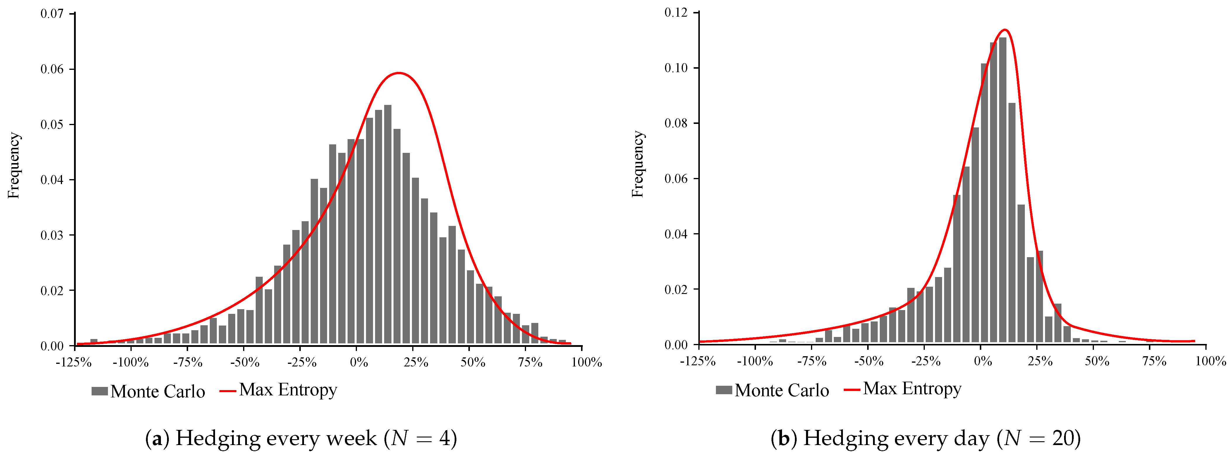
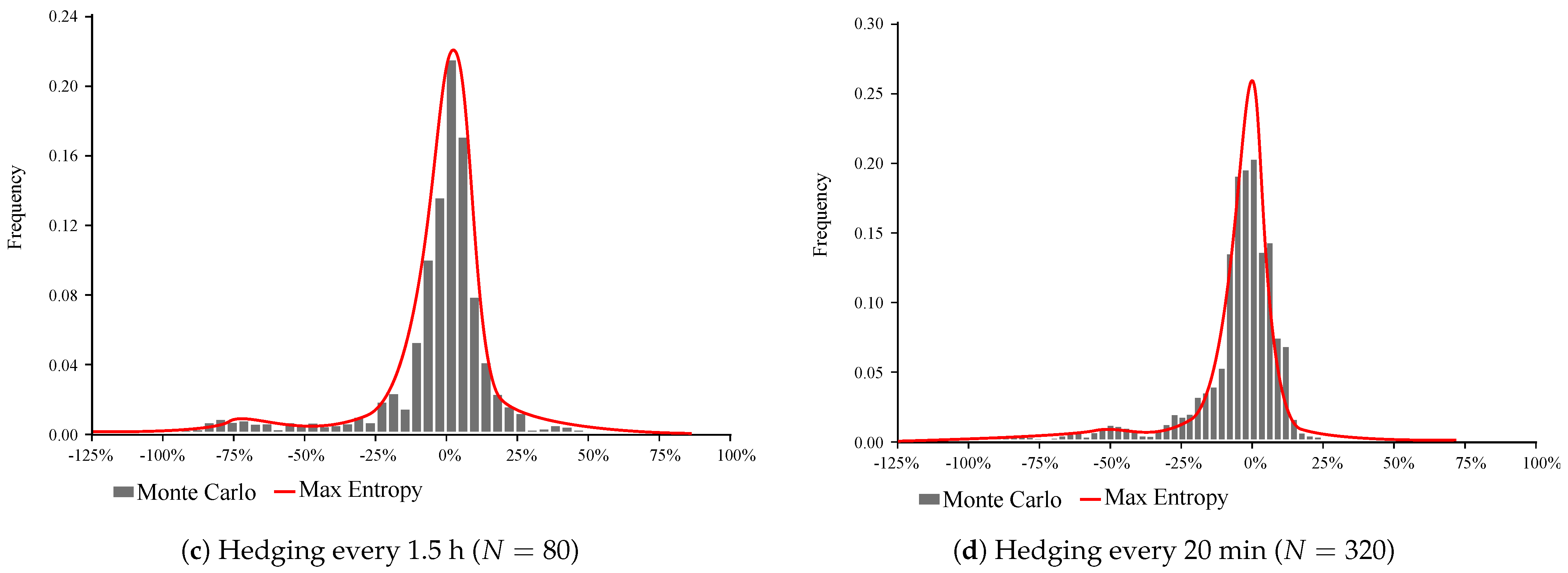
Figure 1 compares the distribution of hedging error obtained from the Monte Carlo Simulation and estimated from the ME method. In
Table 1 we report the summary statistics for the distribution of hedging error, as well as the 99% and 95% VaR, obtained by the above two methods. From the numerical analysis, it follows that the distribution of hedging error for a small number of trades has a high volatility and is negatively skewed, which indicates that it is more likely to have large losses than large wins. It is noteworthy that the ME estimation of the distribution fails to sufficiently capture the right tail of the empirical distribution, nevertheless it adequately describes the left tail.
As we increase the frequency of the delta hedging trades, the distribution becomes more symmetric, and our ME estimation performs better. For , our distribution is strongly leptokurtic, indicating the option writers’ large exposure to jumps. When trading frequency increases to 80 and 320, the distribution peaks around zero and the volatility significantly decreases, however, the left tail is still noticeable. From our analysis, it appears that the volatility is negatively related to the frequency of delta hedging trades. However, further research is required to conclusively establish the relationship between the number of trades and moments of the distributions.


