
Modeling and Simulating Cross Country Banking Contagion Risks


1
Department of Economics and Business Sciences, University of Cagliari, Via S. Ignazio 17, 09123 Cagliari, Italy
2
Department of Accountancy, Bentley University, 175 Forest Street, Waltham, MA 02452, USA
*
Author to whom correspondence should be addressed.
J. Risk Financial Manag. 2021, 14(8), 351; https://0-doi-org.brum.beds.ac.uk/10.3390/jrfm14080351
Submission received: 28 June 2021
/
Revised: 25 July 2021
/
Accepted: 27 July 2021
/
Published: 31 July 2021
(This article belongs to the Special Issue The Future of Banking Risk and Regulation)
Abstract
:The recent financial crisis proved that financial contagion could spread among countries resulting in disruptive effects. In this paper, by modeling and simulating banking system behavior and linkages across countries, we assess, based on data from the BIS and IMF, the possible outcome of domestic crises and how contagion spreads over countries. Results allow detailing the role of a “lighter” or of a “fueler” of financial crises for each country and assessing how each country can affect each other country by contagion, signaling the importance of financial interdependence between some neighboring countries, and detailing which counterpart country would be affected by the ring-fencing of each considered country’s banking system. The method also allows for what-if analyses to optimize the risk exposures, and to plan an emergency strategy in case of alarms coming from specific countries.
JEL Classification:
G01; G17; G15; G211. Introduction and Literature Review
The recent financial crises proved that, as banking systems are interrelated, financial contagion can spread among banks and countries, resulting in disruptive effects.
Analyses devoted to financial contagion have explored two main approaches. The first approach is based on balance sheet values and exposures, so including almost all banks, and aims at verifying how the balance sheet equilibriums of the considered banks would impact on banking system stability. In this way, it is possible to link the micro regulation (at single bank level) to the system effects, allowing supervisors and regulators to assess how macroprudential regulation would affect system stability (see, e.g., European Commission 2014). The second approach is based on market values, which, on the one hand, allow for a timely evaluation of early warning signals (Holopainen and Sarlin 2017), and on the other hand limits its application to listed banks, typically large, so not giving a correct picture of the whole system.
In this paper, we follow the first approach. The literature on this topic, starting from the seminal paper of Allen and Gale (2000), reports that two components are fundamental in determining contagion risks, namely correlation and exposures.
Contagion occurs when the financial distress of a single bank affects one bank’s ability to pay debts to other financial institutions. Interbank exposures have a fundamental role because, if a troubled bank does not repay its obligations to the other banks, the impact can compromise the solvency of its creditor banks and start a domino effect that spreads through the banking system, possibly impacting the whole financial system and, beyond that, the health of the entire economy.
Correlation also plays a fundamental role in contagion risk. If banks tend to react in the same way to the business cycle and common external shocks, the system is then exposed to fewer but more intense crises that impact more banks simultaneously.
These two components, correlation, and exposures, affect system (in)stability in an interrelated way. In fact, correlation mainly sets the favorable conditions for contagion to start, while exposures are the channels through which the crises propagate from one troubled entity to the others, leading to further weakening or defaults.
Theoretical studies have applied network theory to banking systems and focused on the specific characteristics of the interbank matrix structure. Allen and Gale (2000) considered a banking system with different lending structures. Their analysis distinguished between “complete” structures where every bank has direct exposure to all the other banks and “incomplete” structures where some banks are not directly linked to any other bank. Furthermore, they identified “connected” structures, where each bank is, at least indirectly, linked to one another, and “disconnected” structures, and showed that, for any given shock, some structures would lead to contagion while others would not. More network analysis results, as in Brusco and Castiglionesi (2007) and Hasman and Samartin (2008), show that “incompletely connected” structures have higher resilience to contagion effects, since “disconnected” structures are more prone to contagion than “complete” structures, but the latter prevent contagion from spreading to all banks. Looking at empirical approaches, Upper (2011) summarizes the papers focusing on the role played by the interbank market in spreading financial contagion, all of which are based on simulations, due to the limited number of crises reporting contagion cases.
Other studies, such as Battiston et al. (2012), Elliott et al. (2014), and Acemoglu et al. (2015), confirm that the system resilience is related to the interbank market topological structure.
These studies confirm that the interbank matrix structure plays a fundamental role in determining contagion risks, but it is not publicly available when dealing with banks or banking groups, where bank-to-bank exposure mapping is only available to supervisors.
In this paper, instead, we focus on the interrelations among countries’ banking systems and the country-to-country exposures coming from the BIS, which significantly improves the quality of contagion estimates.
A second stream of the literature focuses its attention on the actual assessment of default risks, and places higher attention on bank characteristics, such as dimension, capitalization, and asset riskiness, which evidently play a role not only in determining the banks’ weakness, but also in supporting contagion risks.
In this direction, the contribution of Zedda and Cannas (2020), after estimating each bank’s risk contribution, quantified the impact of the characteristics of banks on contagion risks, proving that interbank exposures (positive) and capital coverage (negative) are the main drivers of contagion risk contributions. In this case, no specific attention is given to the interbank matrix structure, which is estimated based on the maximum entropy hypothesis.
With specific reference to the Monte Carlo simulation of banking systems, the main references in the literature are the models developed by Elsinger et al. (2006), De Lisa et al. (2011) and Drehmann and Tarashev (2013). A complete and in-depth review of the literature on this topic is in Zedda (2017).
The Elsinger et al. (2006) model bases its simulation on the market value of listed banks and then inverting the European call option pricing formula (with maturity fixed to one year) to derive the riskiness of the banks’ assets. They then simulate the system performances assuming that the banks’ asset portfolio returns are normally distributed. Correlation is included in the model by drawing the same quantile of each bank’s average default frequency distribution. Finally, the interbank matrix is approximated by the maximum entropy hypothesis for the unknown bank-to-bank exposures.
Like the other models based on market values, this approach can only be applied to banks whose shares are traded in stock exchanges, so it is typically not applied to small banks. This limit is more evident when considering that simulations are always system-dependent and that the small banks’ balance sheets, equilibriums, and business models are typically different from the larger ones so that the simulation of a system consisting only of large banks can lead to biased results.
The second model, proposed in De Lisa et al. (2011), is known as SYMBOL (SYstemic Model of Banking Originated Losses) and was initially used for Deposit Guarantee Schemes dimensioning. Since then the model has been used both for scientific analyses (see e.g., Galliani and Zedda 2015; Zedda and Sbaraglia 2020; Zhang et al. 2020; Parrado-Martínez et al. 2019) and repeatedly applied by the European Commission for the ex-ante impact assessment of several legislative proposals (for instance, Marchesi et al. 2012), to estimate the impact of financial crises on public finances (see European Commission 2011a, 2011b; Zedda et al. 2012), and back testing the effects of the new European regulation (European Commission 2014). The model is based on the simulation of shocks coming from credit risk, and on the subsequent accounting for direct contagion through interbank lending. An important feature of this model is that it is only based on balance sheet data, so it can be applied to all banks and not only to the listed ones. Even in this model, the interbank exposures are estimated through the maximum entropy hypothesis, and the correlation among banks’ results is set at 50% for all banks.
The Drehmann and Tarashev (2013) model for evaluating the systemic risk contribution of banks developed an approach similar to Elsinger et al. (2006) with Monte Carlo simulated common shocks, based on setting the idiosyncratic and common shocks variance–covariance matrix, in order to have an a posteriori default rate coherent with the estimates of the banks’ probability of default as published by rating agencies. Shocks are partially common and partially idiosyncratic. Here the interbank matrix is also estimated based on the total bank exposures and on the maximum entropy. The limits of this approach, due to the fact that it is based on ratings data, are similar to those of market-based measures.
In this paper, we further developed the SYMBOL model to apply it to countries’ banking systems instead of single banks. So, coherently with the original model, we keep the shocks coming from credit risk, and include direct interbank lending as contagion channel, without any reference to market data.
As for the previous papers, our adaptation brings some loss of quality in data approximation because it considers countries banks’ total assets and capitalization instead of single values for each bank, so using a proxy of the average country value and losing the specificity of each bank. Some previous studies examined the risks of cross-border bank contagion, e.g., Gropp et al. (2009) for Europe, but due to the banking system complexity (in 2008, the European banking system included more than 8000 banks1) the system had to be proxied by a sample of 40 banks. The simplification of considering the whole national banking system as one single entity is equivalent to the approximation we make when considering one bank risk as determined by the average of its assets portfolio, i.e., to hypothesize the same (average) riskiness for all assets, the same capitalization, and the same correlation level.
Conversely, the data publicly available within the BIS database includes country-to-country exposures (also by sector), which gives a much more detailed evaluation of the actual exposures and the possible interbank contagion channeling. We thus adapted the model for including the additional information coming from this source.
A second enhancement of the model is in setting a specific value for each country’s shocks correlation. Regarding the common risk sources, as reported by the literature, credit risk is mainly linked to GDP variations, while financial market correlation both includes local shock effects and impulse-response effects. When dealing with financial markets data, the correlation of shocks can be proxied by stock market indices (Forbes and Rigobon 2002), credit-to-GDP gaps or house prices gaps which are found to be leading indicators of financial crises (Andries and Sprincean 2021). When, instead, the research is based on balance sheet data, as in this paper, the main references can be found in the analyses of Demirgüç-Kunt and Huizinga (2000) and Bikker and Hu (2002) which suggest that bank profitability is related to the business cycle, and of Karimzadeh et al. (2013) whose results showed that bank yields, risk, and loan losses are strictly related to the yearly changes in GDP. Following these references, we set the correlation among country shocks as proxied by the same countries’ GDP correlation, as detailed in the next section.
The third adaptation consists of a smoother contagion mechanism. In the original model, contagion is based on a step effect, as each single bank either defaults and spreads losses to the counterparts or does not default. When dealing with countries, instead, the outcome of a crisis is smooth, and typically some bank would default while others would not, so the spreading losses cannot be modeled as a fixed share of the interbank debts of the whole country, but must consider the crisis dimension, resulting in an endogenous estimation of the system Loss Given Default (LGD).
With these changes, the new model keeps the original model approach and adapts it to the new problem to obtain a proxy of the countries’ risk of domestic banking default and the risk of inducing or suffering from contagion. The resulting model allows the assessment of international interbank contagion risks and the performance of what-if analyses on the impact of one country ring-fencing, or limiting one country so it would not lend to other countries or borrow from other countries.
Based on the simulation model described above, we performed a more in-depth analysis of the contagion effects to verify the role of each considered country in the global crises and assess the effect of each country’s risks on every other country.
This exercise is performed similarly to the Leave-One-Out approach, first proposed in Zedda and Cannas (2020) which is based on the idea that the marginal effects of each considered entity on systemic risk can be obtained by comparing the performance of the entire system with the performance of the same system when excluding (or ring-fencing) the entity under consideration.
In this way, we can address the question of which countries contribute most to starting a crisis (playing the role of a crisis lighter) and which countries are likely to sustain financial contagion (fueling the crisis), detailing each country’s risk contribution and its effects on other countries, providing significant information for supervision and regulation.
Furthermore, we verified the effect of limiting each country’s international banking activity to avoid the country’s lending or borrowing from other countries.
Results show that contagion risks are significant, and the details of the point-to-point exposures allow the assessment of which country’s risk affects every other country, providing significant information for system supervision. On the one hand, this assessment allows verification of whether the exposures are in line with expectations and the strategic planning, and on the other hand it allows testing for the effects of any variation in capitalization or exposures, and the evaluation of which effects can come from the variation of other parameters, to help in setting the emergency plan for dealing with possible risks coming from any country.
2. Methodology
The analysis is developed by a Monte Carlo simulation, which includes the representation of each country’s banking system through its dimension (in terms of Total Assets), assets riskiness, capitalization, and exposures (in terms of interbank lending from and borrowing to every other country). Shocks are correlated to verify the effectiveness of contagion on scenarios as closely as possible to the real banking system situation.
As anticipated in the introduction, the model used for this exercise is based on the SYMBOL model2, adapted for its application to countries instead of single banks, including three main innovations.
The first innovation is the setting of the shock correlation as specific for each considered country, estimated on the basis of the country’s GDP variation correlation with respect to the world GDP variation.
Thus, posing as the GDP of country i at time t, and as the world GDP at time t, and noting the variations as we have:
The correlation index for country i, , is obtained as follows:
The second and third innovations refer to contagion modeling.
The obtained correlation index is used in Drehmann and Tarashev (2013) and in Frey and Hledik (2014) for combining an idiosyncratic shock, specific for each considered country, and a common shock, so as to include the effects of common risk sources, of macro variables, and of the business cycle.
Formally, each simulated shock is obtained as follows:
where the common factor just reports the j index, as this is common to all entities considered in simulation j, while the idiosyncratic shock is different for every entity i and every simulation j.
Within Equation (3) the weight of the common factor is , while represents the weight of the idiosyncratic factor . To visualize the two shocks’ composition, one can think of the common shock as the world pandemic outcome, or as the effect of crude oil price variation, which affects the whole world economy, and the idiosyncratic shock as a domestic shock, due, e.g., to a national currency rate significant variation or reduced public spending, which induces a reduction in the national GDP.
Similarly to the previous literature (Elsinger et al. 2006; De Lisa et al. 2011; Drehmann and Tarashev 2013), on each simulation, the losses of each country’s banking system are compared with their capitalization, and countries’ banking systems are considered to be in distress whenever the simulated losses bring the i country below its banking minimum capital requirement , which is set as 8% of its Risk Weighted Assets, or RWA3.
As the total capital is given by the sum of the minimum capital requirement, , plus the excess capital, , we have:
and the country is considered to be in distress as soon as:
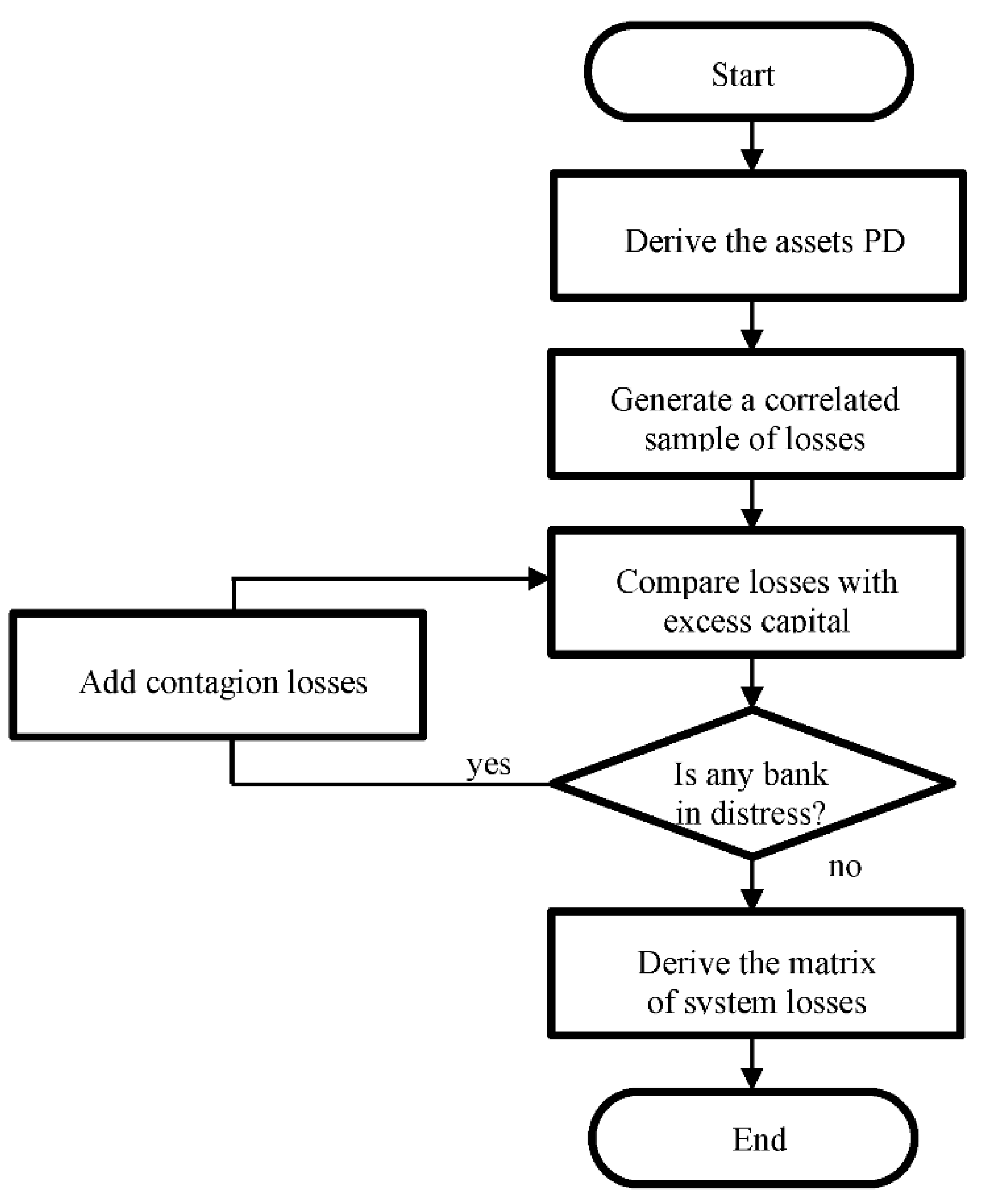
Contagion is then simulated, passing a share of the interbank debts of the defaulted country as losses to the counterpart countries. The share is proportional to the reduction in the MCR suffered by the distressed country. So, a country with 130 billion USD of total capital, of which 100 bn. Is MCR and 30 bn. is EXC, after suffering a loss of, say, 70 bn. will have a residual of 60 bn., with a reduction of capital of 40 bn. below its MCR, and, thus, passing a loss of 40 bn. of its exposures to the creditor countries, which will be spread to each counterpart on the basis of its exposure share. In this evolution, as the country-to-country exposures are known, as measured by the BIS (as in Giudici et al. 2020; Elliott et al. 2014), the attribution of losses can be based on the actual exposure to each counterpart and the interbank exposures can be mapped by means of a matrix. Whenever this additional loss makes a creditor country’s banking system in distress, a share of its interbank debts is passed to the counterpart countries, and the process goes on until it brings another country’s banking systems to distress (as per Equation (5)), as in the Furfine (2003) sequential algorithm. The final losses for each country in each simulation are obtained as the total value of losses above capital for each distressed country and set to zero for non-failed countries. Figure 1 depicts the model flowchart.
To obtain a reliable result in terms of the probability distribution, simulations are performed so as to have 100,000 cases with at least one default, which required around 7.46 million simulations.
3. Data and Results
The model is applied to a sample of countries selected on the basis of data availability. The main source of our data are the BIS international banking statistics, which include values on the country’s banking system dimension, capitalization, and exposures. Exposures are detailed as domestic and foreign, and the foreign exposures are detailed by counterpart country and by counterpart sector. Thus, it is possible to obtain the matrix of country-to-country banking exposures, which, as reported in the introduction, is a key reference for correctly estimating contagion risks.
The second data source are the IMF financial soundness indicators, which report the value of each country’s Risk Weighted Assets (RWAs) needed for proxying the country’s assets riskiness in terms of the country’s average assets’ Probability to Default, PD. Finally, correlation values are obtained from the IMF GDP series, as the correlation between the year-to-year GDP variations of the considered country and the same values for the whole world from 2015 to 2019. The resulting values, referring to the end of 2019, are reported in Table 1, where the assets PD is the average probability to default of the banks’ customers, obtained by inverting the Basel II FIRB formula (see Appendix A for details), and the excess capital is the difference between the actual capital and the minimum capital requirement.
Table 2 reports each country’s foreign interbank exposures, data coming from the BIS, as of end 2019.
The output data are obtained by setting the simulation procedure to record 100,000 cases with one default, which needed 7,461,093 simulations, and resulted in 126,884 primary defaults (before contagion), and a total of 137,335 defaults, including the ones deriving from contagion. Table 3 reports the risk contributions, computed as the total estimated losses divided by the number of simulations.
The values in Table 3 show that the USA is the leading risk contributor before contagion, followed by Switzerland and Korea, and, on average, contagion risks have a minor effect, even if some countries seem significantly exposed to this risk, as in the case of Ireland, Belgium, France, UK, and Singapore.
Previous studies explained this effect by the role of exposures, which make the more exposed countries more prone to contagion. They also highlight that contagion estimates include important complexity, and in some cases, entities not suffering from contagion can induce contagion to other entities involved in the simulation exercise.
One possible representation of these effects can be obtained by measuring the role of “lighter” of crises, i.e., the tendency to start financial crises, which can be measured by the stand-alone contribution, , and the role of “fueling” crises, i.e., to support contagion coming from crises already started, as measured by the contagion risk contribution.
The results reported in Table 3 show the possible “lighter” role of the US, Switzerland, and Korea, which pair a high value for the idiosyncratic risk contribution with a low role in contagion. Instead, other countries can have a highly significant role in supporting contagion risks (crises fuelers), such as Ireland, Belgium, France, the UK, and Singapore.
Other significant results come from the detailed analysis of which country’s exclusion (or ring-fencing) affects each counterpart country’s risk contribution, reported in Table 4 where the risk contribution of each country (rows) is reported as a result of the ring-fencing of one country (column), or of avoiding its foreign lending (Table 5) or its foreign borrowing (Table 6).
As expected, the first evidence of this is that the effect of ring-fencing of one country (Table 4) is in the cells on the main diagonal (from upper left to lower right), where the risk contribution of the ring-fenced country comes back to its stand-alone contribution, so scoring a significant reduction for the “fueler” countries (see, e.g., Ireland). What is less expected is that, in other cases, the exclusion of one country (e.g., UK) induces important reductions in the risk contribution of another country (e.g., Ireland).
Similar cases are of France affecting Finland and Ireland. These cases are probably due to the solid financial linkages between these countries, which are in geographical proximity and are economically linked.
The ring-fencing considered for the previous exercise involves both the exclusion of lending and borrowing from other countries. In fact, we can split the previous effect into its two components, the exclusion of lending to other countries (Table 5) and the exclusion of borrowing from other countries (Table 6).
In the first case (no foreign lending), the not-lending country would not suffer from losses coming from other countries, so the contagion effect is wiped out in the considered country, due to the ring-fencing, resulting in a significant reduction in the values on the main diagonal., Other interesting effects can be evidenced, particularly the effect of the UK not lending to Ireland, Finland, Sweden, and Belgium, bringing more risk for these countries.
In the second case, the most significant effects are for the USA not borrowing from Ireland, Finland, and Sweden, which significantly reduces contagion risks for these countries.
The previous analyses, detailing the effect of each country’s lending or borrowing from each other country, add novel information on country-to-country relationships. These results are of significant importance for banking system supervision, as the knowledge of which countries can bring financial instability risks allows more focused monitoring of the risks and gives some examples of the expected effects of the reduction in the banks’ interlinkages to each counterpart country.
4. Economic Discussion and Conclusions
In this paper, we analyzed the risk contribution of banking systems through a Monte Carlo simulation, taking into consideration national banking systems as single entities and assessing their role in systemic crises, both when considering and not considering financial contagion. Results show that the risk contributions before and after contagion can be different, as contagion risks are significant.
The comparison of results when ring-fencing one country, or excluding its international lending and borrowing, adds important information. It describes each country’s role as “a lighter” or “a fueler” of financial crises, and allows assessment of which countries are affected by contagion risks from other countries, which signals the importance of financial interdependence between some neighboring countries and defines which counterpart country would be affected by the ring-fencing of each considered country’s banking system.
The distinction between countries responsible for starting a crisis, and those only involved in a crisis as a consequence of contagion effects, allows for a more focused supervision.
As reported in Zedda and Cannas (2020), the two risks are driven by different variables. The risk related to primary distress (crisis lighter) is mainly driven by the assets’ riskiness and capitalization levels, so it can be mitigated by raising the minimum capital requirements for the supervised banking system, and monitored for the counterpart countries by periodically measuring these variables. Contagion risks, such as the risk of becoming a crisis fueler, is instead strictly linked to exposures, whose role is analyzed in depth in this paper by means of Monte Carlo simulations, in which contagion effects are specifically modeled, and not just estimated as results of market data, so as to allow verification of the effects of each variation in the exposures’ matrix.
These results add significant information and allow for more focused policy interventions. The higher approximation of risk sources allows monitoring and prevention of contagion risks and verifying if contagion risks are concentrated in some specific country. Moreover, it allows to verification of whether the actual interdependence and exposure to risks are in line with expectations and strategical planning. In case the risk value and distribution among countries are not in line with expectations, it is also possible to verify which changes allow reaching the expected equilibrium, by means of focused what-if tests, similar to those in this paper. The same approach can be applied to assess the expected effects of new exposures, due, e.g., to mergers or acquisitions realized by foreign banking groups, which typically bring significant exposures to the host institution, and so to its home country. In this case, the exercise will be similar, but of the opposite sign, testing for the effects of higher exposure to the acquiring bank’s home country.
Another use of the methodology presented here is in case of alarms coming from any early warning system about financial risks coming from a specific country. In this case, the method can be used to develop what-if analyses, for assessing the possible effects of reducing or closing any financial exposure to the risky country, and planning the emergency strategy by assessing which of the alternative financial sources is coming from less risky countries, and those less exposed to the risky ones.
The approach can be refined by regulators and supervisors, who have access to confidential data on bank-to-bank exposures. With these data, they can perform a similar exercise with higher precision, and arrive at a more complete estimation of contagion effects by considering the indirect contagion channels, i.e., the possible effects of short-selling in case of financial crises, which can suddenly reduce the market value of some assets (e.g., sovereign bonds). These weakening effects would add to the initial crisis and to the direct contagion of weakening effects, significantly worsening the framework (Zedda 2015). These indirect contagion effects have not been explored in this paper, due to the unavailability of the necessary data, which are instead available to supervisors, as disclosed by the EBA for some European countries4.
Finally, the results reported in this paper, and the methodology developed for obtaining them, add new tools and can be useful for regulators and supervisors to lower the risk of financial crises spreading across countries, to react to incoming crises properly, and to keep the financial system safe and sound.
Author Contributions
Conceptualization, S.Z.; methodology, S.Z.; data curation, A.S.-C.; writing: S.Z. and A.S.-C. Both authors have read and agreed to the published version of the manuscript.
Funding
This research received no external funding.
Institutional Review Board Statement
Not applicable.
Informed Consent Statement
Not applicable.
Conflicts of Interest
The authors declare no conflict of interest.
Appendix A. The SYMBOL Model
The first step in the SYMBOL model is the estimation of the riskiness of each bank’s credit portfolio.
This estimation is based on the minimum capital requirement FIRB formula (Basel II Foundation Internal Ratings-Based function for credit risk, see Basel Committee on Banking Supervision 2005, 2006, 2010, 2013), which states that the minimum capital requirement for each bank is given by the sum of the capital allocation parameter Cik for each exposure k in the portfolio of bank i multiplied by its amount Aik:
where the capital allocation parameter (Cik) for each exposure k in the portfolio of bank is given by:
where:
is the probability of default of the loan k in the portfolio of bank i
is the loss given default of the same loan;
is the maturity of loan k;
is the size of the counterpart firm for loan k;
N(x) is the normal cumulative density function and N−1(x) is its inverse function;
and
A proxy of each bank’s credit portfolio riskiness denoted by , can be obtained by numerical inversion of the FIRB formula, on the base of the bank’s minimum capital requirements and total assets value, and setting the other parameters contained in the Basel FIRB function, i.e., loss given default (LGD), maturity (M) and size (S), to their standard values:
As a second step, the estimated credit portfolio riskiness are used as to generate a set of calibrated losses , correlated across the system, on the base of the same FIRB formula modified so to replace the 0.999 value, set for determining the confidence level of 99.9%, with the random variable .
So, the estimated losses are generated by the following formula:
where
are the countries’ indexes;
identify each simulation run;
are correlated normal random shocks.
| 1 | Source: ECB. |
| 2 | See the Appendix A for details. |
| 3 | The New York University Stern School Vlab SRISK documentation reports that “By default, the prudential capital requirement used in calculating such capital shortfalls is set to be 8% for firms in Africa, Asia and Americas and 5.5% for firms in Europe due to differences in accounting standards” (https://vlab.stern.nyu.edu/docs/srisk (accessed on 27 June 2021)). The scientific literature instead typically sets the minimum capital requirement to 8%, see, e.g., Brownlees and Engle (2017), Berger et al. (2019), and Chen et al. (2021) thus we kept this setting as reference for the estimations. |
| 4 | See the EBA 2020 EU-wide transparency exercise, in which for every bank in the sample is reported the exposure to each counterpart country, detailed by maturity classes. https://www.eba.europa.eu/risk-analysis-and-data/eu-wide-transparency-exercise (accessed on 27 June 2021). |
References
- Acemoglu, Daron, Asuman Ozdaglar, and Alireza Tahbaz-Salehi. 2015. Systemic risk and stability in financial networks. American Economic Review 105: 564–608. [Google Scholar] [CrossRef]
- Allen, Franklin, and Douglas Gale. 2000. Financial contagion. Journal of Political Economy 108: 1–33. [Google Scholar] [CrossRef]
- Andries, Alin Marius, and Nicu Sprincean. 2021. Cyclical behaviour of systemic risk in the banking sector. Applied Economics 53: 1463–97. [Google Scholar] [CrossRef]
- Basel Committee on Banking Supervision. 2005. An Explanatory Note on the Basel II IRB Risk Weight Functions. Available online: https://www.bis.org/bcbs/irbriskweight.pdf (accessed on 27 June 2021).
- Basel Committee on Banking Supervision. 2006. International Convergence of Capital Measurement and Capital Standards. Available online: https://www.bis.org/publ/bcbs128.pdf (accessed on 27 June 2021).
- Basel Committee on Banking Supervision. 2010. A Global Regulatory Framework for More Resilient Banks and Banking Systems. Available online: https://www.bis.org/publ/bcbs189_dec2010.pdf (accessed on 27 June 2021).
- Basel Committee on Banking Supervision 2013. Revised Basel III Leverage Ratio Framework and Disclosure Requirements. Available online: https://www.bis.org/publ/bcbs270.pdf (accessed on 27 June 2021).
- Battiston, Stefano, Domenico Delli Gatti, Mauro Gallegati, Bruce Greewald, and Joseph E. Stiglitz. 2012. Liaisons dangereuses: Increasing connectivity, risk sharing, and systemic risk. Journal of Economic Dynamics and Control 36: 1121–41. [Google Scholar] [CrossRef] [Green Version]
- Berger, Allen N., Raluca A. Roman, and John Sedunov. 2019. Did TARP reduce or increase systemic risk? The effects of government aid on financial system stability. Journal of Financial Intermediation 43: 100810. [Google Scholar] [CrossRef]
- Bikker, Jacob, and H aixia Hu. 2002. Cyclical Patterns in Profits, Provisioning and Lending of Banks. DNB Staff Reports, No. 86. Amsterdam: De Nederlandsche Bank. [Google Scholar]
- Brownlees, Christian, and Robert F. Engle. 2017. SRISK: A conditional capital shortfall measure of systemic risk. The Review of Financial Studies 30: 48–79. [Google Scholar] [CrossRef]
- Brusco, Sandro, and Fabio Castiglionesi. 2007. Liquidity coinsurance, moral hazard and financial contagion. Journal of Finance 62: 2275–302. [Google Scholar] [CrossRef]
- Chen, Lei, Hui Li, Frank Hong Liu, and Yue Zhou. 2021. Bank regulation and systemic risk: Cross country evidence. Review of Quantitative Finance and Accounting 57: 353–87. [Google Scholar] [CrossRef]
- De Lisa, Riccardo, Stefano Zedda, Francesco Vallascas, Francesca Campolongo, and Massimo Marchesi. 2011. Modelling Deposit Insurance Schemes’ losses in a Basel 2 framework. Journal of Financial Services Research 40: 123–41. [Google Scholar] [CrossRef]
- Demirgüç-Kunt, Asli, and Harry Huizinga. 2000. Financial Structure and Bank Profitability. Policy Research Working Paper Series 2430; Washington: The World Bank. [Google Scholar]
- Drehmann, Mathias, and Nikola Tarashev. 2013. Measuring the systemic importance of interconnected banks. Journal of Financial Intermediation 22: 586–607. [Google Scholar] [CrossRef] [Green Version]
- Elliott, Matthew, Benjamin Golub, and Matthew O. Jackson. 2014. Financial network and contagion. American Economic Review 104: 3115–53. [Google Scholar] [CrossRef] [Green Version]
- Elsinger, Helmut, Alfred Lehar, and Martin Summer. 2006. Using market information for banking system risk assessment. International Journal of Central Banking 2: 137–65. [Google Scholar] [CrossRef] [Green Version]
- European Commission. 2011a. Directorate-General for Economic and Financial Affairs, Public Finances in EMU 2011, European Economy 3. Available online: https://ec.europa.eu/economy_finance/publications/european_economy/2011/pdf/ee-2011-3_en.pdf (accessed on 27 June 2021).
- European Commission. 2011b. Directorate-General for Internal Market and Services: Commission Staff Working Document—Impact Assessment Accompanying the Proposal for a Directive of the European Parliament and of the Council Establishing a Framework for the Recovery and Resolution. Available online: https://www.eumonitor.eu/9353000/1/j9vvik7m1c3gyxp/vk9idfnk1qrb (accessed on 27 June 2021).
- European Commission. 2014. Directorate-General for Internal Market and Services, Commission Staff Working Document—Economic Review of the Financial Regulation Agenda. Available online: https://eur-lex.europa.eu/legal-content/EN/TXT/HTML/?uri=CELEX:52014SC0158&from=fr (accessed on 27 June 2021).
- Forbes, Kristin J., and Roberto Rigobon. 2002. No contagion, only interdependence: Measuring stock market comovements. The Journal of Finance 57: 2223–61. [Google Scholar] [CrossRef]
- Frey, Rüdiger, and Juraj Hledik. 2014. Correlation and Contagion as Sources of Systemic Risk, SSRN. Available online: http://ssrn.com/abstract=2541733 (accessed on 27 June 2021).
- Furfine, Craig H. 2003. Interbank exposures: Quantifying the risk of contagion. Journal of Money, Credit and Banking 35: 111–28. [Google Scholar] [CrossRef]
- Galliani, Clara, and Stefano Zedda. 2015. Will the bail-in break the vicious circle between banks and their sovereign? Computational Economics 45: 597–614. [Google Scholar] [CrossRef]
- Giudici, Paolo, Peter Sarlin, and Alessandro Spelta. 2020. The interconnected nature of financial systems: Direct and common exposures. Journal of Banking and Finance 112: 105–49. [Google Scholar] [CrossRef]
- Gropp, Reint, Marco Lo Duca, and Jukka Vesala. 2009. Cross-border bank contagion in Europe. International Journal of Central Banking 5: 97–139. [Google Scholar]
- Hasman, Augusto, and Margarita Samartin. 2008. Information acquisition and financial contagion. Journal of Banking & Finance 32: 2136–47. [Google Scholar]
- Holopainen, Markus, and Peter Sarlin. 2017. Toward Robust Early-Warning Models: A Horse Race, Ensembles and Model Uncertainty. Quantitative Finance 17: 1–31. [Google Scholar] [CrossRef]
- Karimzadeh, Majid, S. M. Jawed Akhtar, and Behzad Karimzadeh. 2013. Determinants of profitability of banking sector in India. Transition Studies Review 20: 211–19. [Google Scholar] [CrossRef]
- Marchesi, Massimo, Marco Petracco Giudici, Jessica Cariboni, Stefano Zedda, and Francesca Campolongo. 2012. Macroeconomic Cost-Benefit Analysis of Basel III Minimum Capital Requirements and of Introducing Deposit Guarantee Schemes and Resolution Funds. Eur—Scientific and Technical Research Series; Luxembourg: European Commission Publication Office, ISBN 978–92-79-17781-1. [Google Scholar]
- Parrado-Martínez, Purificación, Pilar Gómez-Fernández-Aguado, and Antonio Partal-Ureña. 2019. Factors influencing the European bank’s probability of default: An application of SYMBOL methodology. Journal of International Financial Markets, Institutions and Money 61: 223–40. [Google Scholar] [CrossRef]
- Upper, Christian. 2011. Simulation methods to assess the danger of contagion in interbank markets. Journal of Financial Stability 7: 111–25. [Google Scholar] [CrossRef]
- Zedda, Stefano. 2015. Direct vs. side effects in financial contagion: What weights more? In Advances in Artificial Economics, Lecture Notes in Economics and Mathematical Systems. Edited by Frédéric Amblard, Francisco J. Miguel, Adrien Blanchet and Benoit Gaudou. Cham: Springer, vol. 676, pp. 131–38. [Google Scholar]
- Zedda, Stefano. 2017. Banking Systems Simulation: Theory, Practice, and Application of Modeling Shocks, Losses, and Contagion. Hoboken: John Wiley & Sons. [Google Scholar]
- Zedda, Stefano, and Giuseppina Cannas. 2020. Assessing banks’ systemic risk contribution and contagion determinants trough the leave-one-out approach. Journal of Banking and Finance 112: 105160. [Google Scholar] [CrossRef]
- Zedda, Stefano, and Simone Sbaraglia. 2020. Which interbank net is the safest? Risk Management 22: 65–82. [Google Scholar] [CrossRef]
- Zedda, Stefano, Jessica Cariboni, Massimo Marchesi, Marco Petracco Giudici, and Matteo Salto. 2012. The EU Sovereign Debt Crisis: Potential Effects on EU Banking Systems and Policy Options. Eur—Scientific and Technical Research Series; Luxembourg: European Commission Publication Office. [Google Scholar]
- Zhang, Xiaoming, Chunyan Wei, and Stefano Zedda. 2020. Analysis of China commercial banks’ systemic risk sustainability through the leave-one-out approach. Sustainability 12: 203. [Google Scholar] [CrossRef] [Green Version]
Figure 1.
Simulation flowchart.


Table 1.
Countries’ banking systems data as of 2019.
| Country | Assets PD % | Excess Capital US$ bn. | Total Assets US$ bn. | Correlation |
|---|---|---|---|---|
| Australia | 0.002125 | 87.4 | 2890.5 | 0.682 |
| Austria | 0.002055 | 49.5 | 840.4 | 0.500 |
| Belgium | 0.001357 | 19.8 | 560.4 | 0.688 |
| Canada | 0.001243 | 141.2 | 4755.0 | 0.532 |
| Denmark | 0.000555 | 35.3 | 1066.4 | −0.351 |
| Finland | 0.001082 | 37.4 | 723.1 | 0.551 |
| France | 0.001133 | 289.0 | 7960.4 | 0.672 |
| Germany | 0.001142 | 284.7 | 7990.2 | 0.853 |
| India | 0.002748 | 84.7 | 2290.0 | 0.582 |
| Ireland | 0.002415 | 22.3 | 285.6 | 0.198 |
| Italy | 0.001895 | 129.4 | 3130.0 | 0.827 |
| Japan | 0.000616 | 680.5 | 20,857.3 | 0.574 |
| Korea | 0.003001 | 75.2 | 2345.0 | 0.933 |
| Netherlands | 0.001017 | 96.0 | 2616.8 | 0.889 |
| Portugal | 0.002239 | 18.3 | 304.8 | 0.636 |
| Singapore | 0.002640 | 54.5 | 1024.0 | 0.976 |
| Spain | 0.001775 | 156.1 | 3877.8 | 0.468 |
| Sweden | 0.000810 | 38.6 | 926.2 | 0.427 |
| Switzerland | 0.001894 | 71.4 | 3032.5 | 0.667 |
| United Kingdom | 0.001020 | 285.2 | 7420.8 | 0.334 |
| United States | 0.004232 | 759.3 | 14,903.3 | 0.248 |
The table reports the input values for the considered banking systems in terms of assets riskiness, capitalization dimension and GDP correlation, showing that the major differences are in the system dimension.
Table 2.
Countries’ banking systems foreign exposures (US$ bn.).
| Australia | Austria | Belgium | Canada | Denmark | Finland | France | Germany | India | Ireland | Italy | Japan | Korea | Netherlands | Portugal | Singapore | Spain | Sweden | Switzerland | United Kingdom | United States | |
|---|---|---|---|---|---|---|---|---|---|---|---|---|---|---|---|---|---|---|---|---|---|
| Australia | 0 | 18 | 238 | 3190 | 57 | 527 | 16,995 | 9629 | 9048 | 502 | 196 | 12,370 | 3783 | 2832 | 80 | 12,864 | 763 | 212 | 954 | 56,633 | 25,542 |
| Austria | 186 | 0 | 387 | 2597 | 1321 | 970 | 15,313 | 26,399 | 1361 | 556 | 2164 | 242 | 44 | 1600 | 11 | 24 | 2668 | 593 | 4436 | 5261 | 597 |
| Belgium | 602 | 225 | 0 | 3026 | 1182 | 71,338 | 83,592 | 37,481 | 2050 | 2004 | 6473 | 5953 | 634 | 39,662 | 145 | 1313 | 4408 | 745 | 1642 | 45,020 | 9185 |
| Canada | 4465 | 1338 | 3704 | 0 | 1224 | 461 | 28,371 | 31,745 | 1151 | 8650 | 1061 | 2652 | 1090 | 13,941 | 99 | 5487 | 1096 | 1057 | 989 | 96,988 | 85,668 |
| Denmark | 114 | 567 | 787 | 226 | 0 | 15,565 | 14,150 | 15,825 | 38 | 1724 | 259 | 78 | 1 | 668 | 5 | 23 | 888 | 35,873 | 175 | 11,316 | 2459 |
| Finland | 210 | 401 | 528 | 1173 | 12,983 | 0 | 10,792 | 6818 | 29 | 264 | 392 | 87 | 38 | 1012 | 1 | 1 | 219 | 45,560 | 341 | 11,177 | 5067 |
| France | 11,945 | 3506 | 69,783 | 24,768 | 8865 | 8314 | 0 | 124,951 | 28,536 | 31,604 | 162,329 | 108,616 | 7933 | 55,121 | 6564 | 11,242 | 90,326 | 7881 | 44,054 | 248,566 | 157,970 |
| Germany | 13,772 | 35,834 | 9726 | 17,261 | 8324 | 6568 | 293,141 | 0 | 19,982 | 24,837 | 84,979 | 34,661 | 4771 | 87,436 | 185 | 185 | 56,927 | 4647 | 17,261 | 234,695 | 134,718 |
| India | 28,236 | 573 | 1284 | 7489 | 106 | 638 | 25,107 | 14,959 | 0 | 7 | 278 | 54,829 | 24,675 | 7634 | 15 | 46,859 | 1029 | 997 | 5065 | 52,435 | 44,042 |
| Ireland | 789 | 582 | 10,615 | 1491 | 3131 | 264 | 55,575 | 30,737 | 73 | 0 | 38,913 | 328 | 97 | 24,421 | 170 | 142 | 3654 | 1288 | 843 | 67,912 | 24,198 |
| Italy | 258 | 10,303 | 2986 | 1537 | 411 | 774 | 84,116 | 60,329 | 3151 | 12,754 | 0 | 324 | 87 | 13,117 | 92 | 81 | 8608 | 292 | 2934 | 34,560 | 18,615 |
| Japan | 23,608 | 895 | 18,965 | 7519 | 5467 | 1759 | 93,445 | 18,446 | 56,224 | 207 | 8060 | 0 | 9774 | 11,328 | 725 | 48,747 | 2257 | 2059 | 3304 | 125,976 | 213,682 |
| Korea | 1605 | 419 | 145 | 570 | 39 | 1 | 4726 | 2494 | 7955 | 140 | 59 | 8164 | 0 | 507 | 88 | 2101 | 122 | 48 | 232 | 4122 | 23,232 |
| Netherlands | 13,335 | 948 | 31,748 | 9044 | 1031 | 1047 | 105,326 | 51,689 | 25,716 | 28,900 | 15,085 | 2577 | 958 | 0 | 701 | 23,210 | 9338 | 1344 | 12,840 | 183,463 | 28,937 |
| Portugal | 250 | 169 | 191 | 216 | 147 | 82 | 3700 | 453 | 150 | 441 | 62 | 842 | 191 | 238 | 0 | 712 | 3063 | 5 | 377 | 953 | 3836 |
| Singapore | 11,423 | 177 | 639 | 5432 | 18 | 0 | 7492 | 453 | 41,582 | 636 | 54 | 26,620 | 11,251 | 255 | 5795 | 0 | 140 | 529 | 5592 | 24,462 | 29,913 |
| Spain | 363 | 1555 | 3906 | 1971 | 1072 | 302 | 66,157 | 25,495 | 5500 | 6195 | 27,837 | 468 | 430 | 22,036 | 8971 | 813 | 0 | 322 | 3204 | 60,579 | 26,041 |
| Sweden | 329 | 630 | 674 | 1309 | 37,736 | 51,749 | 8046 | 8971 | 333 | 2520 | 279 | 2141 | 38 | 3888 | 0 | 0 | 331 | 0 | 1207 | 23,660 | 31,757 |
| Switzerland | 7119 | 3260 | 8320 | 3365 | 2241 | 2642 | 66,650 | 31,745 | 6581 | 4637 | 1955 | 2860 | 1773 | 11,238 | 9 | 5397 | 3038 | 1687 | 0 | 123,352 | 30,874 |
| United Kingdom | 96,838 | 8450 | 31,344 | 144,394 | 13,859 | 15,195 | 452,037 | 268,304 | 43,881 | 102,161 | 43,987 | 279,629 | 11,871 | 158,640 | 2394 | 38,365 | 40,834 | 20,271 | 204,928 | 0 | 391,974 |
| United States | 82,764 | 6292 | 5965 | 92,834 | 1367 | 32,996 | 201,161 | 56,226 | 32,952 | 43,120 | 4088 | 325,041 | 27,368 | 10,276 | 2333 | 27,616 | 16,134 | 52,715 | 10,717 | 324,512 | 0 |
The table reports the international banking claims, detailing how each (column header) country is exposed to every other (row header) country.
Table 3.
Systemic risk contributions (US$ bn.) by country.
| No Contagion | With Contagion | |
|---|---|---|
| Australia | 78.79 | 81.92 |
| Austria | 3.48 | 3.64 |
| Belgium | 4.88 | 6.68 |
| Canada | 53.57 | 54.35 |
| Denmark | 2.45 | 2.45 |
| Finland | 1.39 | 1.66 |
| France | 48.17 | 57.47 |
| Germany | 50.24 | 56.93 |
| India | 59.75 | 65.06 |
| Ireland | 0.55 | 2.13 |
| Italy | 30.65 | 33.73 |
| Japan | 54.20 | 55.73 |
| Korea | 96.25 | 99.56 |
| Netherlands | 12.50 | 15.92 |
| Portugal | 1.35 | 1.44 |
| Singapore | 8.95 | 14.65 |
| Spain | 37.59 | 37.98 |
| Sweden | 2.09 | 2.76 |
| Switzerland | 114.13 | 115.82 |
| United Kingdom | 29.93 | 35.77 |
| United States | 335.10 | 337.44 |
The risk contribution estimates report that the United States is the main risk contributors, while Singapore and the UK show the largest difference from no contagion to contagion contributions.
Table 4.
Variation in countries’ systemic risk contributions when the column header country is isolated (%).
Table 4.
Variation in countries’ systemic risk contributions when the column header country is isolated (%).
| Australia | Austria | Belgium | Canada | Denmark | Finland | France | Germany | India | Ireland | Italy | Japan | Korea | Netherlands | Portugal | Singapore | Spain | Sweden | Switzerland | United Kingdom | United States | |
|---|---|---|---|---|---|---|---|---|---|---|---|---|---|---|---|---|---|---|---|---|---|
| Australia | −4% | 0% | 0% | 0% | 0% | 0% | 1% | 0% | 0% | 0% | 0% | 1% | −1% | 0% | 0% | 0% | 0% | 0% | 0% | 2% | 1% |
| Austria | 0% | −4% | 0% | 0% | 0% | 0% | 3% | −2% | 0% | 0% | −1% | 0% | −1% | 0% | 0% | 0% | 0% | 0% | 0% | 2% | 1% |
| Belgium | 1% | 0% | −27% | 0% | 0% | 0% | −5% | 1% | 2% | 1% | 2% | −2% | −1% | −3% | 0% | 1% | 2% | 0% | −2% | 20% | 14% |
| Canada | 0% | 0% | 0% | −1% | 0% | 0% | 1% | 0% | 0% | 0% | 0% | 1% | 0% | 0% | 0% | 0% | 0% | 0% | 0% | 1% | 0% |
| Denmark | 0% | 0% | 0% | 0% | 0% | 0% | 0% | 0% | 0% | 0% | 0% | 0% | 0% | 0% | 0% | 0% | 0% | 0% | 0% | 1% | 0% |
| Finland | 4% | 0% | −1% | 5% | 3% | −16% | 17% | 4% | 2% | 2% | 0% | 32% | 1% | 1% | 0% | 1% | 1% | −6% | 0% | 36% | −12% |
| France | 0% | 0% | 0% | 1% | 0% | 0% | −16% | −3% | 1% | 1% | −2% | 3% | −2% | 0% | 0% | 0% | 0% | 0% | −2% | 9% | 5% |
| Germany | −1% | 0% | 0% | 0% | 0% | 0% | 2% | −12% | 0% | 0% | −3% | 1% | −2% | −1% | 0% | 0% | 0% | 0% | −1% | 5% | 4% |
| India | 0% | 0% | 0% | 0% | 0% | 0% | 2% | 0% | −8% | 0% | 0% | 0% | −4% | 0% | 0% | −2% | 0% | 0% | 0% | 3% | 7% |
| Ireland | 12% | 2% | 3% | 14% | 1% | 5% | 49% | 5% | 7% | −74% | −4% | 76% | 2% | −2% | 0% | 4% | 4% | 7% | 1% | 71% | −42% |
| Italy | 0% | 0% | 0% | 0% | 0% | 0% | −1% | −4% | 0% | 0% | −9% | 1% | 0% | 0% | 0% | 0% | 0% | 0% | 0% | 5% | 2% |
| Japan | 0% | 0% | 0% | 0% | 0% | 0% | 1% | 0% | 0% | 0% | 0% | −3% | −1% | 0% | 0% | 0% | 0% | 0% | 0% | 2% | 2% |
| Korea | 0% | 0% | 0% | 0% | 0% | 0% | 0% | 0% | −1% | 0% | 0% | 0% | −3% | 0% | 0% | −1% | 0% | 0% | 0% | 1% | 1% |
| Netherlands | −1% | 1% | 0% | 0% | 0% | 0% | 5% | −8% | 0% | 1% | −2% | 1% | −1% | −21% | 0% | 0% | 0% | 0% | −1% | 8% | 7% |
| Portugal | 0% | 0% | 0% | 0% | 0% | 0% | 1% | 0% | 2% | 0% | 0% | 1% | −1% | 0% | −6% | −4% | −1% | 0% | 0% | 4% | 3% |
| Singapore | −5% | 0% | 1% | 1% | 0% | 0% | 8% | 2% | −5% | 0% | 0% | −3% | −9% | −2% | 0% | −39% | 0% | 0% | −1% | 18% | 22% |
| Spain | 0% | 0% | 0% | 0% | 0% | 0% | 0% | 0% | 0% | 0% | 0% | 0% | 0% | 0% | 0% | 0% | −1% | 0% | 0% | 0% | 0% |
| Sweden | 6% | 0% | 0% | 7% | 0% | 1% | 20% | 5% | 2% | 3% | 0% | 39% | 2% | 1% | 0% | 2% | 1% | −24% | 1% | 38% | −23% |
| Switzerland | 0% | 0% | 0% | 0% | 0% | 0% | 0% | 0% | 0% | 0% | 0% | 0% | 0% | 0% | 0% | 0% | 0% | 0% | −1% | 0% | 1% |
| United Kingdom | 1% | 0% | 1% | 2% | 0% | 1% | 10% | 0% | 1% | 1% | 0% | 14% | 0% | −1% | 0% | 1% | 1% | 1% | −2% | −16% | 1% |
| United States | 0% | 0% | 0% | 0% | 0% | 0% | 0% | 0% | 0% | 0% | 0% | 0% | 0% | 0% | 0% | 0% | 0% | 0% | 0% | 0% | −1% |
The estimations allow assessment of how the exclusion of one country form the system would affect each counterpart country.
Table 5.
Variation in countries’ systemic risk contributions when the column header country is not lending to other countries (%).
Table 5.
Variation in countries’ systemic risk contributions when the column header country is not lending to other countries (%).
| Australia | Austria | Belgium | Canada | Denmark | Finland | France | Germany | India | Ireland | Italy | Japan | Korea | Netherlands | Portugal | Singapore | Spain | Sweden | Switzerland | United Kingdom | United States | |
|---|---|---|---|---|---|---|---|---|---|---|---|---|---|---|---|---|---|---|---|---|---|
| Australia | −4% | 0% | 0% | 0% | 0% | 0% | 1% | 0% | 0% | 0% | 0% | 2% | 0% | 0% | 0% | 0% | 0% | 0% | 0% | 2% | 2% |
| Austria | 0% | −4% | 0% | 0% | 0% | 0% | 3% | 1% | 0% | 0% | 0% | 0% | 0% | 0% | 0% | 0% | 0% | 0% | 0% | 2% | 1% |
| Belgium | 1% | 0% | −27% | 1% | 0% | 0% | 6% | 5% | 3% | 1% | 4% | 4% | 0% | 0% | 0% | 2% | 2% | 0% | 1% | 20% | 14% |
| Canada | 0% | 0% | 0% | −1% | 0% | 0% | 1% | 0% | 0% | 0% | 0% | 1% | 0% | 0% | 0% | 0% | 0% | 0% | 0% | 1% | 0% |
| Denmark | 0% | 0% | 0% | 0% | 0% | 0% | 0% | 0% | 0% | 0% | 0% | 0% | 0% | 0% | 0% | 0% | 0% | 0% | 0% | 1% | 0% |
| Finland | 5% | 0% | 0% | 6% | 3% | −16% | 18% | 5% | 2% | 2% | 1% | 32% | 1% | 1% | 0% | 2% | 1% | −6% | 1% | 36% | 3% |
| France | 1% | 1% | 0% | 1% | 0% | 0% | −16% | 3% | 1% | 1% | 0% | 5% | 0% | 1% | 0% | 1% | 1% | 0% | 0% | 9% | 7% |
| Germany | 0% | 0% | 0% | 0% | 0% | 0% | 4% | −12% | 1% | 0% | 0% | 1% | 0% | 0% | 0% | 0% | 0% | 0% | 0% | 5% | 4% |
| India | 1% | 0% | 0% | 0% | 0% | 0% | 2% | 1% | −8% | 0% | 0% | 2% | 0% | 0% | 0% | −1% | 0% | 0% | 0% | 3% | 7% |
| Ireland | 14% | 2% | 3% | 16% | 1% | 5% | 57% | 17% | 7% | −74% | 2% | 78% | 4% | 2% | 0% | 5% | 5% | 7% | 4% | 73% | 16% |
| Italy | 0% | 0% | 0% | 0% | 0% | 0% | 2% | 1% | 0% | 0% | −9% | 1% | 0% | 1% | 0% | 0% | 1% | 0% | 0% | 5% | 3% |
| Japan | 0% | 0% | 0% | 0% | 0% | 0% | 1% | 0% | 0% | 0% | 0% | −3% | 0% | 0% | 0% | 0% | 0% | 0% | 0% | 2% | 2% |
| Korea | 0% | 0% | 0% | 0% | 0% | 0% | 1% | 0% | 0% | 0% | 0% | 1% | −3% | 0% | 0% | 0% | 0% | 0% | 0% | 1% | 1% |
| Netherlands | 1% | 1% | 0% | 1% | 0% | 0% | 9% | 2% | 1% | 1% | 1% | 2% | 0% | −21% | 0% | 0% | 1% | 0% | 0% | 8% | 7% |
| Portugal | 0% | 0% | 0% | 0% | 0% | 0% | 2% | 1% | 2% | 0% | 1% | 1% | 0% | 0% | −6% | −1% | 0% | 0% | 0% | 4% | 3% |
| Singapore | 2% | 0% | 1% | 1% | 0% | 0% | 9% | 3% | 2% | 0% | 1% | 7% | 1% | 0% | 0% | −39% | 0% | 0% | 0% | 18% | 23% |
| Spain | 0% | 0% | 0% | 0% | 0% | 0% | 0% | 0% | 0% | 0% | 0% | 0% | 0% | 0% | 0% | 0% | −1% | 0% | 0% | 1% | 0% |
| Sweden | 6% | 0% | 0% | 7% | 1% | 1% | 20% | 5% | 2% | 3% | 0% | 39% | 2% | 1% | 0% | 2% | 1% | −24% | 1% | 38% | 1% |
| Switzerland | 0% | 0% | 0% | 0% | 0% | 0% | 0% | 0% | 0% | 0% | 0% | 0% | 0% | 0% | 0% | 0% | 0% | 0% | −1% | 0% | 1% |
| United Kingdom | 2% | 0% | 1% | 3% | 0% | 1% | 13% | 4% | 2% | 1% | 1% | 16% | 1% | 1% | 0% | 1% | 1% | 1% | 0% | −16% | 9% |
| United States | 0% | 0% | 0% | 0% | 0% | 0% | 0% | 0% | 0% | 0% | 0% | 1% | 0% | 0% | 0% | 0% | 0% | 0% | 0% | 0% | −1% |
The estimations allow assessment of how the lending restrictions to one country would affect each other country. The most significant effects refer to the UK and Japan.
Table 6.
Variation in countries’ systemic risk contributions when the column header country is not borrowing from other countries (%).
Table 6.
Variation in countries’ systemic risk contributions when the column header country is not borrowing from other countries (%).
| Australia | Austria | Belgium | Canada | Denmark | Finland | France | Germany | India | Ireland | Italy | Japan | Korea | Netherlands | Portugal | Singapore | Spain | Sweden | Switzerland | United Kingdom | United States | |
|---|---|---|---|---|---|---|---|---|---|---|---|---|---|---|---|---|---|---|---|---|---|
| Australia | 0% | 0% | 0% | 0% | 0% | 0% | 0% | 0% | −1% | 0% | 0% | 0% | −1% | 0% | 0% | −1% | 0% | 0% | 0% | 0% | −1% |
| Austria | 0% | 0% | 0% | 0% | 0% | 0% | 0% | −2% | 0% | 0% | −1% | 0% | −1% | 0% | 0% | 0% | 0% | 0% | 0% | 0% | 0% |
| Belgium | −1% | 0% | 0% | −1% | 0% | 0% | −12% | −4% | 0% | 0% | −2% | −6% | −1% | −5% | 0% | −1% | 0% | 0% | −3% | −1% | −1% |
| Canada | 0% | 0% | 0% | 0% | 0% | 0% | 0% | 0% | 0% | 0% | 0% | 0% | 0% | 0% | 0% | 0% | 0% | 0% | 0% | 0% | −1% |
| Denmark | 0% | 0% | 0% | 0% | 0% | 0% | 0% | 0% | 0% | 0% | 0% | 0% | 0% | 0% | 0% | 0% | 0% | 0% | 0% | 0% | 0% |
| Finland | 0% | 0% | −2% | 0% | 0% | −1% | −1% | −1% | 0% | 0% | 0% | 0% | 0% | 0% | 0% | 0% | 0% | −7% | −1% | −1% | −13% |
| France | −1% | 0% | −1% | 0% | 0% | 0% | −2% | −6% | −1% | 0% | −3% | −1% | −2% | −2% | 0% | −1% | −1% | 0% | −2% | −1% | −2% |
| Germany | −1% | 0% | 0% | −1% | 0% | 0% | −2% | −2% | 0% | 0% | −4% | 0% | −2% | −1% | 0% | 0% | 0% | 0% | −2% | −1% | 0% |
| India | −1% | 0% | 0% | 0% | 0% | 0% | 0% | −1% | −1% | 0% | 0% | −2% | −4% | 0% | 0% | −2% | 0% | 0% | 0% | 0% | 0% |
| Ireland | −2% | 0% | 0% | −2% | 0% | 0% | −9% | −10% | −1% | −1% | −8% | −1% | −2% | −7% | 0% | −1% | −1% | −1% | −3% | −11% | −57% |
| Italy | 0% | 0% | 0% | 0% | 0% | 0% | −4% | −5% | 0% | 0% | 0% | 0% | 0% | −1% | 0% | 0% | −1% | 0% | 0% | 0% | 0% |
| Japan | 0% | 0% | 0% | 0% | 0% | 0% | 0% | 0% | 0% | 0% | 0% | −1% | −1% | 0% | 0% | −1% | 0% | 0% | 0% | 0% | −1% |
| Korea | −1% | 0% | 0% | 0% | 0% | 0% | 0% | 0% | −1% | 0% | 0% | 0% | 0% | 0% | 0% | −1% | 0% | 0% | 0% | 0% | 0% |
| Netherlands | −1% | 0% | −1% | −1% | 0% | 0% | −4% | −10% | −1% | 0% | −3% | −1% | −2% | −1% | 0% | 0% | −1% | 0% | −2% | −1% | 0% |
| Portugal | 0% | 0% | 0% | 0% | 0% | 0% | −1% | 0% | 0% | 0% | 0% | 0% | −1% | 0% | 0% | −4% | −2% | 0% | 0% | 0% | 0% |
| Singapore | −7% | 0% | 0% | −1% | 0% | 0% | −1% | −1% | −9% | 0% | 0% | −9% | −10% | −3% | 0% | −1% | 0% | 0% | −2% | 0% | −1% |
| Spain | 0% | 0% | 0% | 0% | 0% | 0% | 0% | 0% | 0% | 0% | 0% | 0% | 0% | 0% | 0% | 0% | 0% | 0% | 0% | 0% | 0% |
| Sweden | 0% | 0% | 0% | 0% | 0% | −2% | 0% | 0% | 0% | 0% | 0% | 0% | 0% | 0% | 0% | 0% | 0% | 0% | 0% | −1% | −23% |
| Switzerland | 0% | 0% | 0% | 0% | 0% | 0% | 0% | 0% | 0% | 0% | 0% | 0% | 0% | 0% | 0% | 0% | 0% | 0% | 0% | 0% | 0% |
| United Kingdom | −2% | 0% | 0% | −1% | 0% | 0% | −3% | −4% | −1% | −1% | −1% | −2% | −1% | −2% | 0% | −1% | 0% | 0% | −2% | 0% | −8% |
| United States | 0% | 0% | 0% | 0% | 0% | 0% | 0% | 0% | 0% | 0% | 0% | 0% | 0% | 0% | 0% | 0% | 0% | 0% | 0% | 0% | 0% |
The estimations allow assessing how the borrowing restrictions to one country would affect each other country. The most significant effects refer to the US.
Publisher’s Note: MDPI stays neutral with regard to jurisdictional claims in published maps and institutional affiliations. |
© 2021 by the authors. Licensee MDPI, Basel, Switzerland. This article is an open access article distributed under the terms and conditions of the Creative Commons Attribution (CC BY) license (https://creativecommons.org/licenses/by/4.0/).
Share and Cite
MDPI and ACS Style
Zedda, S.; Spinace-Casale, A. Modeling and Simulating Cross Country Banking Contagion Risks. J. Risk Financial Manag. 2021, 14, 351. https://0-doi-org.brum.beds.ac.uk/10.3390/jrfm14080351
AMA Style
Zedda S, Spinace-Casale A. Modeling and Simulating Cross Country Banking Contagion Risks. Journal of Risk and Financial Management. 2021; 14(8):351. https://0-doi-org.brum.beds.ac.uk/10.3390/jrfm14080351
Chicago/Turabian StyleZedda, Stefano, and Antonella Spinace-Casale. 2021. "Modeling and Simulating Cross Country Banking Contagion Risks" Journal of Risk and Financial Management 14, no. 8: 351. https://0-doi-org.brum.beds.ac.uk/10.3390/jrfm14080351