
The Skewness Risk in the Energy Market


Department of Accountancy and Finance, Otago Business School, University of Otago, Dunedin 9054, New Zealand
*
Author to whom correspondence should be addressed.
J. Risk Financial Manag. 2021, 14(12), 620; https://0-doi-org.brum.beds.ac.uk/10.3390/jrfm14120620
Submission received: 29 October 2021
/
Revised: 6 December 2021
/
Accepted: 11 December 2021
/
Published: 20 December 2021
(This article belongs to the Special Issue Energy Finance and Sustainable Development)
Abstract
:In this paper, we study the skewness risk and its return predictability in the energy market. Skewness risk is often used to measure the possibility of market crash. We study both physical skewness (market skewness and cross-sectional average realized skewness) estimated from underlying stock returns and risk-neutral skewness evaluated from the options market. We find a significant positive relationship between one-month-ahead market return and average realized skewness in the energy market. This unique feature should be noted by investors and carefully considered by energy policymakers.
JEL Classification:
G12; G171. Introduction
Intro1 START1 The change in the energy market condition reflects economic shocks that are often captured by the skewness of energy-related asset returns during times of massive oil price movement. Skewness risk is often used to measure the possibility of a market crash. Oil price fluctuations also often result from a demand shift in the sources of energy that effectively influence the performance of energy stocks (Hamilton 1983; Van Hoang et al. 2019; Gagnon and Power 2020). Studying the skewness or crash risk in predicting future returns has been extensively explored at the individual and market level in the existing literature. For example, skewness risk (both based on realized and risk-neutral measures) predicts future equity and options returns (Amaya et al. 2015; Byun and Kim 2016; Da Fonseca and Xu 2017; Long et al. 2019; Atilganet al. 2019).1 Although a large volume of research has been carried out on studying skewness risk, there have been a limited number of empirical investigations into the relationship between skewness risk and energy-related equity returns; therefore, studying the crash risk in the energy market, which captures the aggregate sensitivity of individual energy stocks returns concerning their price changes over time, is our important current work.
This study examines skewness risk and its return predictability in the energy market by creating its own energy market index (EMI), which tracks the Energy Select Sector SPDR ETF (XLE). To date, the XLE is one of the largest energy ETFs, among others, and also the first energy sector–concentrated ETF in the US. This is the first paper focusing on the energy market to examine the predictability of both physical skewness (market skewness and cross-sectional average realized skewness) estimated from energy stock returns and risk-neutral skewness evaluated from the energy options. The study follows theoretical frameworks by Goyal and Santa-Clara (2003) and Bali et al. (2005), to provide empirical evidence that the cross-sectional average skewness helps to predict subsequent (risk-adjusted) energy market returns. We further adapt the methodology from Ruan and Zhang (2018, 2019) to study nonparametric risk-neutral skewness in the energy sector. We find a significant positive relationship between one-month-ahead market return and average realized skewness in the energy market. That is, a one-standard-deviation increase in the average skewness results, on average, in a 0.54% (=0.06 × 0.0903) increase in the energy market excess return the next month.
Additionally, the results also hold with the inclusion of several economic control variables. These include default spread, term spread, the average correlation across all energy stocks, implied volatility of energy market index (XLE), and the variance risk premium (VRP) that are known to help predict aggregate market returns. The predictability of average energy stock skewness is further tested with the inclusion of an illiquidity measure, and we find that consistent with the baseline regression, the effect of average energy stock skewness remains significant and positive. In the case of using nonparametric risk-neutral variance (NRNV) and skewness (NRNSk) in this study, however, we find an insignificant relationship with the future energy market return.2
Our study contributes to the existing literature primarily by linking individual average skewness to the energy market at the aggregate level. We present a unique relationship between the skewness of individual energy stock returns (derived from the return of individual distribution of the energy stocks) and expected energy market returns. Specifically, we find the average realized skewness (of energy stocks) positively predicts subsequent energy market returns. This outcome is contrary to that of Goyal and Santa-Clara (2003); Bali et al. (2005) and Jondeau et al. (2019), who study the impact of the average skewness risk in the overall stock market. These results, however, reflect those of Stilgeret al. (2016) and Mohrschladt and Schneider (2021), who also find a positive link between skewness risk and future stock returns,3 though our empirical evidence primarily stems from average realized skewness. The evidence from this study suggests that realized skewness is an important driver of subsequent energy market returns, while skewness risk implied by options is not. The findings of this study have a number of important implications for future practice; therefore, investors in the energy market should be aware of this unique feature and it should be carefully considered by energy policymakers. For example, market participants should pay attention to the effect of the skewness of energy stock prices, as the relationship between the skewness of energy return and equity premium from other assets enables investors to form more diverse equity portfolios by using energy-related assets to hedge against risks. Policymakers could make use of our findings when forming effective hedging strategies to mitigate the impact of oil price shocks on energy-related stocks. Potential policy implications could be motivating companies to efficiently manage the usage of the main source of energy and to support alternative sources to effectively hedge downside risk in energy stock prices. Thus, policymakers should develop a dynamic policy system to handle the risk arising from the unsteady energy market.
2. Literature Review
LiteratureStarts A large strand of the literature uses skewness risk to capture the possibility of market crashes and relates this factor to future individual or market returns. The aspect of the skewed distribution of underlying returns has received at least two competing views. Bali et al. (2009); Huang et al. (2012) and Gennaioli et al. (2013) argue that preference for higher skewness captures the gambling behavior of investors, while others, such as Kelly and Jiang (2014); Bollerslev et al. (2015); Long et al. (2019) and Dertwinkel-Kalt and Köster (2019) view it as a source of tail risk. Modeling such dynamics of irrational randomness in stock prices dates back to Press (1967) and Merton (1976), who propose a model for the distribution of changes in stock prices and derive an option pricing formula for the more general case with the underlying security returns, respectively; however, previous research exploring the relationship between skewness risk and energy market returns is rather scarce.
In early years, Merton (1976) argued that the loss-aversion utility is frequently used to express the role of unsystematic volatility and the role of idiosyncratic skewness. The author finds that in an economy with investors who are loss averse, only with regard to the movements of individual stocks that they own, their stock returns tend to be high, on average, excessively risky, and can observe large cross-sectional premiums by a commonly used multi-factor model. In recent years, Mitton and Vorkink (2007) show that investors who favor positive skewness diversify their portfolio less to have more exposure in underlying assets with positive unsystematic skewness. The study suggests, as a result and at equilibrium, stocks with large unsystematic skewness often pay a reward. Kumar (2009) finds that investors’ tendency to bet on a gamble and their investment decisions are closely related. Boyer et al. (2009) find expected unsystematic skewness and returns are negatively correlated.
Xing et al. (2010) and Yan (2011) find implied volatility smirk factors significantly predict future stock returns. Chang et al. (2013) and Conrad et al. (2013) use higher moments of market returns to see whether these factors explain the cross-sectional variation in individual stock returns. Stilger et al. (2016) use risk-neutral skewness to predict the future market return and equity returns. Bali et al. (2019) examine the relationship between implied volatility, skewness, kurtosis, and ex-ante cross-sectional equity returns and find a significant and positive predictive power from all three moments. Jondeau et al. (2019) use realized skewness to predict the future market returns and equity returns. More recently, Mohrschladt and Schneider (2021) find short-lived predictability of out-of-the-money (OTM) based model-free option-implied skewness (MFIS) using common ordinary US stocks for their sample period. The authors also find predictability of MFIS significantly reverses when in-the-money (ITM) options are used instead.
Although a large volume of research has studied skewness risk, there have been a limited number of empirical investigations into the relationship between skewness risk and energy-related equity returns; therefore, studying the crash risk in the energy market, which captures aggregate sensitivity of individual energy stock returns concerning their price changes over time, is our important current work.
Another strand of literature studies the link between energy-related underlying or commodity return and the equity market. Studying these links dates back to Hamilton (1983) and Gilbert and Mork (1984), who find that the economic recession is highly related to oil price shocks.
The economic recession affects the overall equity market as a whole, which also can be seen in the recent financial crisis periods, such as the 2000 dot-com bubble and the 2008 financial crisis, respectively. Ciner (2013) examines the relationship between changes in oil price and equity returns in the US, and finds significant time variation in the link between oil and other equity prices. The author finds the impact of oil price shocks that persist less than 12 months on stock returns is negative and significant. The paper also observes a joint-movement of the stock market and oil prices. More recently, Maghyereh et al. (2016) find that the bulk of interconnection is predominantly governed by the transmission of information from the oil market to equity markets but not vice versa. Van Hoang et al. (2019) and Chuliáet al. (2019) present the existence of a spillover effect in the energy market in the US and Europe, respectively. Gagnon and Power (2020) find skewness and tail risks are locally driven in Brent and WTI oil indexes and suggest that these two indices can be used for hedging extreme risks during market disruptions. Dutta et al. (2020) study how equity investors in clean energy markets can reduces their downside risk. Specifically, the authors examine the roles of the commodity market volatility indexes of crude oil, gold, and silver. The authors find that the volatility indexes of these commodities provide effective hedging that reduce their downside risk. Dawaret al. (2021) examine the relationship between crude oil and renewable energy stock prices by employing a quantile-based regression approach. The authors suggest that clean energy stock returns react differently to new information on oil returns under different market conditions. By analyzing the asymmetrical effect of oil returns on clean energy stock returns, they find a strong effect of negative oil returns during bearish periods.
In this paper, we study the skewness risk and its return predictability in the energy market. Skewness risk is often used to measure the possibility of market crash. Unlike the standing literature, we study both physical skewness (market skewness and cross-sectional average realized skewness) estimated from underlying stock returns and risk-neutral skewness evaluated from options market.
Our study contributes to the existing literature primarily by linking individual average skewness to the energy market at the aggregate level. We present the unique relationship between skewness of individual energy stock returns (derived from the return of individual distribution of the energy stocks) and expected energy market returns. Specifically, we find the average realized skewness (of energy stocks) positively predicts subsequent energy market returns. This outcome is contrary to that of Goyal and Santa-Clara (2003); Bali et al. (2005) and Jondeau et al. (2019), who study the overall stock market. These results reflect those of Stilger et al. (2016) and Mohrschladt and Schneider (2021), who also find a positive link between skewness risk and future stock returns,4 though our empirical evidence primarily stems from average realized skewness.
3. Data
3.1. Energy Market Index (EMI)
EMISTART XLE is the first energy-sector-concentrated ETF in the US that tracks the index of the US energy companies in the S&P 500 and is considered as the largest energy ETF to date. XLE was launched in December 1998 to provide a high volume of exposure to a basket of US companies in the energy sector with a small amount of holding costs (Ruan and Zhang 2019). Because State Street Global Advisors, the issuer of XLE ETF, does not report the list of securities held in its ETF, we create our own energy market index (EMI) which tracks the performance of the XLE ETF very closely. XLE has net assets under management of $9.98 billion, and the average daily trading volume of XLE is around 14.84 million as of the 18th of November 2019.5 The correlation between XLE and EMI is as high as 98% and is used for all model specifications in Section 5. Given the size and growing interest in its market, it is important to study the role of skewness (crash) risk in the energy market to provide information to investors, who seek to invest in commodity or energy-related equity portfolios and for effective risk management.
3.2. The Energy Market Return and Average Factors
Daily energy stock returns are downloaded from the Center for Research in Security Prices (CRSP) for the sample period ranging from January 1996 to December 2018.6 We keep the daily stocks with a share code equal to 10 or 11 and exchange code equal to 1, 2, or 3. We use standard industry classification (SIC) codes to obtain energy sector stocks only and the risk-free rate to compute daily excess returns. The 48 industry classifications for the energy sector are obtained directly from Kenneth French’s website and the risk-free rate is downloaded from CRSP for the sample period, which is the one-month Treasury bill rate.
The initial sample contained 42,775,300 daily observations, and it drops to 900,518 daily observations after applying the above filters. The final sample comprises 494 energy stocks in total. These data are used to compute EMI. Data for the energy market options, such as implied volatility, delta, and days to maturity, are downloaded from IvyDB OptionMetrics matched by their permanent security identifier (PERMNO) and the committee on uniform securities identification procedures (CUSIP) for the sample period of January 1996 to December 2018 and are used to compute nonparametric risk-neutral factors.
3.3. Control Variables
Default Spread
Default spread () is calculated as the difference between a Moody’s Baa corporate bond yield and the ten-year Treasury bond yield.7 The monthly Moody’s corporate bond yield is downloaded directly from the Federal Reserve Bank of St. Louis (FRED) for the sample period ranging from January 1996 to December 2018. The monthly ten-year Treasury bond yield is downloaded from CRSP. is computed using two rates, that is, taking the difference by subtracting the ten-year Treasury bond yield from Moody’s Baa corporate bond yield, which can be defined as
where is the default spread in a current month, t. denotes the monthly Moody’s Baa corporate bond yield at a current month, t, and denotes the monthly ten-year Treasury bond yield at a current month, t.
Term Spread
Term spread () is calculated as the difference between the monthly ten-year Treasury bond yield and three-month Treasury bill rate. is calculated as the difference between the monthly ten-year Treasury bond yield and three-month Treasury bill rate as
where is the term spread in a current month t, and and denote the ten-year Treasury bond and three-month Treasuy bill rate, respectively.
Illiquidity Measure
Illiquidity variable () is calculated using a daily return of energy stocks downloaded from the CRSP dataset, following Amihud (2002) illiquidity measure. The illiquidity of a given stock i in month t is defined as
where is the dollar trading volume of firm i on day d. The aggregate illiquidity is the average across all stocks available in month t:
where denotes the corresponding market capitalization of firm, i, in month, t. We multiply by a million to avoid values being extremely small.
Average Correlation
Average correlation () across all energy stocks is computed using daily returns of energy stocks downloaded from the CRSP dataset for the sample period ranging from January 1996 to December 2018. Following Pollet and Wilson (2010) the number of trading days, , in month t, the sample variance of daily returns for stock j is
where d is a trading day in a month t, and is daily return of stock j at day d.
The sample correlation for stocks j and k, denoted as , is calculated in the usual way given the definition of .
our estimator of , average correlation can be defined as
Implied Volatility
The monthly implied volatility () is computed using daily implied volatilities of XLE index options, only including 30 days to expiration and both call and put options, downloaded from IvyDB OptionMetrics for the sample period ranges from December 1998 to December 2018. is simply the sum of equal-weighted average of daily implied volatilities
where , the average daily implied volatility at month t. d and denote a particular day of the month and total number of days in a month, t, respectively.
Implied Volatility Skew
The skew variable () is the value between the implied volatility of OTM put options and the implied volatility of at-the-money (ATM) call options, which are directly downloaded from IvyDB OptionMetrics for the sample period ranging from January 1996 to December 2017. The days to maturity range from 7 to 186 days, and the minimum (maximum) value of implied volatilities is set to zero (two). The number of days used for calculating historical volatility is set at 30 days. After downloading the value for the sample period, we remove non-energy equity options by matching with the energy stocks’ PERMNO, then take the average for each month across firms. Initially, 323 energy stocks matched for the sample period and then it dropped to 201 energy stock options after removing missing values.
Put-Call-Parity Implied Volatility Spread
Put-call-parity implied volatility spread () is the weighted average of the difference between the implied volatilities of put options and corresponding parity call options, matched by their expiration date and strike price. This variable is directly downloaded from IvDB OptionMetrics for the sample period, from January 1996 to December 2017. The values are only for the energy stocks’ options as they are matched by their PERMNO. Similarly, 323 energy stocks matched and then the number dropped to 303 energy stock options after removing missing values.
Variance Risk Premium
The variance risk premium () of the energy market is simply the difference between the implied volatilities of the XLE index available from IvyDB OptionMetrics and the realized volatility calculated using daily returns of energy stocks from the CRSP dataset for the sample period ranging from December 1998 to December 2018.8 Following Bollerslev et al. (2009) the monthly of the energy market is defined as
where is simply the ex-ante implied volatility of the XLE index options over the time interval and is the realized energy market variance over the time interval. Using the variance differences has the advantage that and , and therefore , are now directly observable at time t.
3.4. Preliminary Analysis
The average monthly EMI return for the entire sample period is 0.0132 with a standard deviation of 0.0561, which is reported in Table 1. The table also reports changes in the EMI return over the sample period. Table 2 shows the summary statistics of the energy sector concerning several available firms and the amount of their total market capitalization over time for both options and stocks. The average total market capitalization of energy stocks and options is $949 and $934 million, respectively. There are 494 and 266 firms available over the sample period for energy stocks and options, respectively. The correlation between EMI and XLE daily return is 98% which is close to 1.9
Table 3 shows the summary statistics and correlation matrix for the following variables: value-weighted CRSP of EMI excess return, , energy market variance, , energy market skewness, , value-weighted average variance, , equal-weighted average variance, , value-weighted average skewness, , and equal-weighted average skewness, , nonparametric risk-neutral volatility, , nonparametric risk-neutral skewness, .
The energy market variance and value-weighted average variance of the energy stocks are both positive, i.e., 0.005 and 0.0072, respectively. The monthly energy market skewness is negative, on average, while average monthly energy stock skewness with equal- and value-weighted measures are positive. Panel B provides a correlation matrix between each variable. EMI return and value- and equal-weighted average energy stock skewness is positively correlated, whereas market variance and nonparametric risk-neutral average variance of the energy stocks are negatively correlated. This may imply that the energy market return decreases (increases) with increases (decreases) in variance risk (skewness risk) of energy stock returns.
Table 4 provides the summary statistics and the correlation matrix of the economic and financial variables under consideration. is a skewness between OTM put and ATM call of the energy sector options, is the put-call-parity implied volatility spread variable of the energy sector options. and are economic control variables and , , , and are financial control variables that we consider in our regression specifications. In Panel A, the mean value of most of the control variables over the sample period are positive on average, apart from —which is −0.0140. , which is the implied volatility of energy stock options—has the highest mean value of 0.2565. Panel B reports the correlation matrix between control variables. Most of control variables have relatively low correlation with each other, ranging from −0.2810 (between and ) to 0.4547 (between and ), apart from a correlation of −0.8616 between and which is considered relatively high. These numbers confirm that the control variables convey the different types of information that is appropriate to be included in testing the robustness of average factors.
4. Methodology
4.1. Theoretical Background of Predictability in Average Variance and Skewness Factors
We adapt the theoretical model of Goyal and Santa-Clara (2003); Bali et al. (2005); and Jondeau et al. (2019),10 which provides assumptions that the expected energy market return should be defined by
where and denote energy market return and risk-free rate for current month t, and denote energy market variance and energy market skewness at a future month, , conditional on the information available at current month, t, and denote average variance and skewness of energy stocks, and is the weight (either based on equal or value), the relative market capitalization of a energy firm i.
4.2. Average Variance and Skewness of the Energy Stocks
Following Jondeau et al. (2019), the individual variance of energy stocks at month t is defined as
where i denotes the energy stock i at month t, d and denote the day in a particular month t and the total number of days in month t. denotes daily individual energy stock i’s excess return and denotes average excess daily return of energy stock i at month t. The average energy stock variance at month t is calculated using either equal weights or value weights, used by Goyal and Santa-Clara (2003) and Bali et al. (2005), respectivley.11
The individual skewness at month t is defined as
where i denotes stock i at month t, d and denote the day in a month t and the total number of days in month t. is based on standardized measure, , is the variance of individual stock i in a month t. The average skewness can also be computed using either value or equal weight, same as the average variance above.
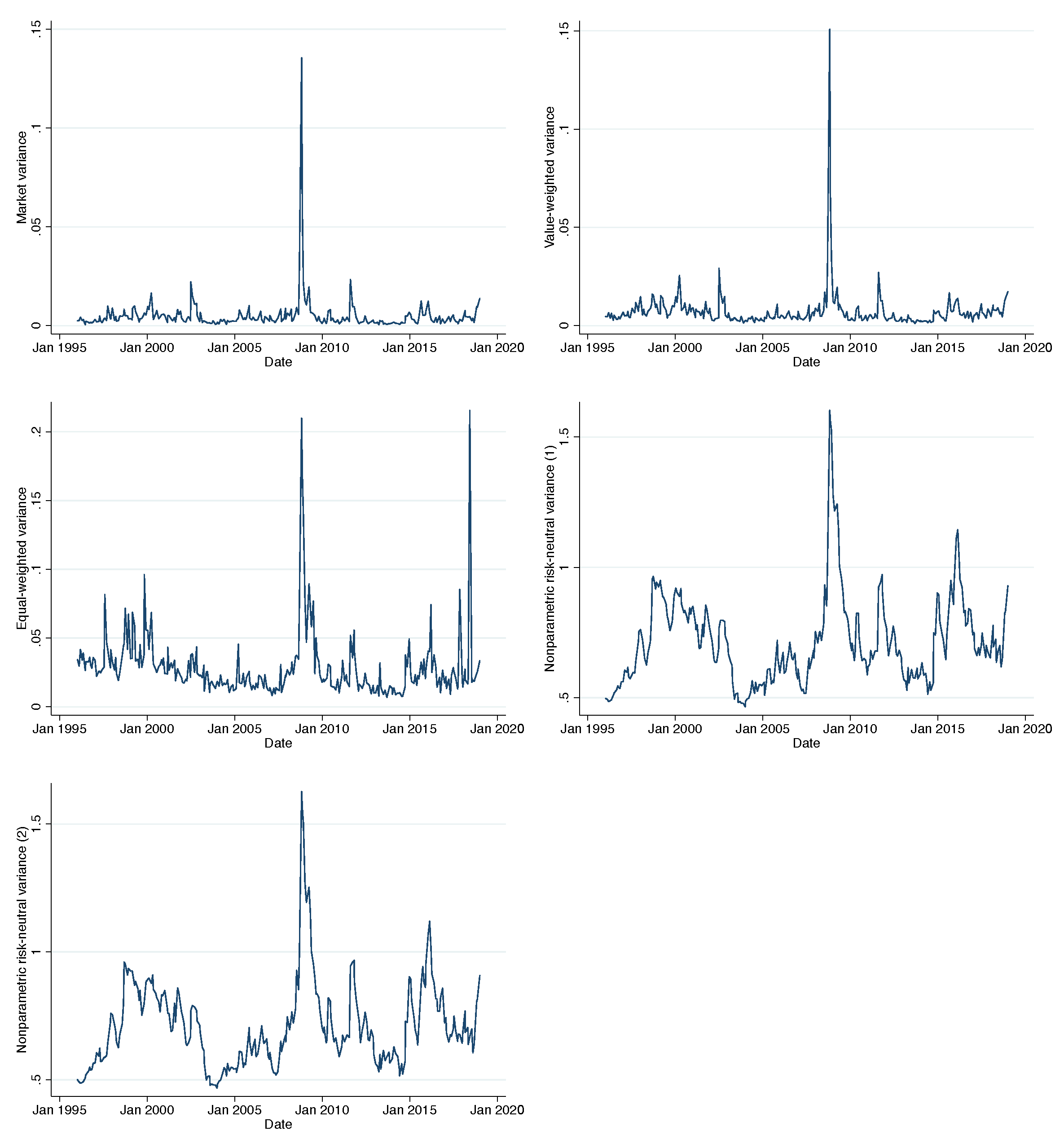
Figure 1 and Figure 2 plot the dynamics of variance and skewness, respectively. The top row in Figure 1 plots the movement of the market and value-weighted variance over time. Interestingly, market variance and value-weighted average variance share similar patterns, unlike market variance with equal-weighted average variance. The value-weighted variance is smoothed out before and after the 2008 global financial crisis but has the highest spike in the same year, which is the same as the other two variance measures (i.e., market and equal-weighted). The last two figures confirm that two average nonparametric risk-neutral volatilities move almost identically.12 This is quite distinct from Jondeau et al. (2019), who observe three different patterns from each variance measure for the overall market index (S&P 500) (i.e., market and two realized average variances).
4.3. Nonparametric Risk-Neutral Moments
Following Xing et al. (2010); Yan (2011); and Ruan and Zhang (2018), NRNV and NRNSk can be defined as
where the implied volatilities of the 50 delta call options () and the delta put options () are the ATM call and put implied volatilities t-day fitted implied volatility surface at time t.13 Similarly, the implied volatility of the 25 delta call options () and the delta put options () are the OTM call and put implied volatilities, respectively.14
The negative relationship between skewness and future equity returns has long been recognized. For instance, Yan (2011) finds that the expected stock return is a function of the average jump size, in the presence of jump risk. This suggests there is a negative predictive relation between the slope of the implied volatility smirk, which is related to risk-neutral skewness, and stock returns. Xing et al. (2010) find that the shape of the implied volatility smirk is known to have statistically and economically significant predictive power, and that the shape of the volatility smirk has significant cross-sectional predictive power for future equity returns. Jondeau et al. (2019) also find that average realized skewness has significant predictability on subsequent market returns. Consistent with the studies mentioned above, we expect to find a consistent result in the US energy market.
5. Empirical Results
This section evaluates the ability of energy market variance and skewness, average realized variance and skewness, and nonparametric risk-neutral variance and skewness to predict the subsequent energy market excess return in the regression corresponding to theoretical expression in Equation (1).
5.1. Baseline Regression
The baseline regression can be written as follows, with the definitions of average variance and skewness based on value- and equal-weights, respectively, and average and based on equal weights:15
where denotes future energy market excess returns, and denote energy market variance and skewness, respectively. and denote either value- or equal-weighted average variance and skewness of energy stock returns, and denote nonparametric average variance and skewness, respectively.
In Table 5, we consider each of the variables in Equations (6) and (7) separately. Panel A reports the results of the regressions for the 1996–2018 sample period using individual variables. The coefficients for market variance and skewness are insignificant as well as all the other average predictors, except for value-weighted average skewness. The value-weighted average skewness has a positive coefficient of 0.006 and is also significant at a conventional level with p-value and adjusted- of 0.046 and 1.11%, respectively. Other variables, including market, average skewness, and equal-weighted variance, have no significant coefficients, which implies that the future energy market excess return cannot be predicted using these variables.
Table 5 Panel B reports the baseline regression of individual variables with the current energy market excess return. The significance of value-weighted average skewness increases slightly with the inclusion of current energy market excess return; however, adjusted- decreases to 0.91%. This means that although the model with current energy market return increases the significance of the value-weighted average skewness factor, the model with value-weighted average skewness as a sole predictor can predict with better precision. Our findings are distinct from the results in many of the existing studies that find significant and negative predictive power in the average skewness factor (Boyer et al. 2009; Conrad et al. 2013; Bali and Murray 2013; Amaya et al. 2015; Byun and Kim 2016; Jondeau et al. 2019); however, our result is consistent, to some extent, with Stilger et al. (2016), who examine the relationship between the risk-neutral skewness of individual stock returns’ distribution obtained from option prices. The study reports a positive relationship between the risk-neutral skewness (RNS), using options, of individual stock returns’ distribution and future realized stock returns during the period from 1996 to 2012.
Table 6 reports predictive regressions of energy market return using a combination of variables. Each specification in Panel A includes variance and skewness at the same time. None of the coefficients is significant in all models inclusive, except for the model with value-weighted average variance and skewness. In Column (2), though it is rather weak, value-weighted skewness positively and significantly predicts subsequent energy market excess return. Panel B in Table 6 reports the baseline regression with a combination of variables with the current energy market excess return. In Column (2) in Panel B, with the inclusion of market factors, the predictive power of value-weighted average skewness is slightly higher than when it used as a sole predictor. The market skewness also has some predictive power in Column (3), where we include equal-weighted average variance and skewness factors. The predictive power in market skewness and equal-weighted skewness may not be as reliable, as they are only significant as additional factor; that is, there was no strong predictability in the market skewness factor alone in predicting subsequent energy market return.
Overall, the results of predictive regression with a combination of variables are consistent with the baseline regression, where we test the predictability of individual variables. The value-weighted skewness has positive predictive power, and it is statistically significant at a 5% level. That is, a one-standard-deviation increase in the average skewness results, on average, in a 0.54% (= 0.0903) increase in the energy market excess return the next month. The results are different from the existing studies that find a negative relationship between the skewness factor and expected stock, market, and options returns (Goyal and Santa-Clara 2003; Bali et al. 2005; Jondeau et al. 2019). However, it is consistent with Stilger et al. (2016), who find a positive relationship between RNS and future equity returns. They argue that this relation is driven by holding stocks that are likely to be over-valued, too risky, or too costly to trade. Further, they find that only the idiosyncratic component of the RNS factor contributes to this relationship, not the systematic part.
5.2. Controlling for the Economic and Financial Variables
In this section, we look at whether the results from baseline regression are robust with the inclusion of the economic and financial variables. Goyal and Santa-Clara (2003) investigate the relationship between market return and average stock variance after controlling for several economic variables.
We consider a similar set of economic variables following Goyal and Santa-Clara (2003). The default spread (), the term spread () as well as the illiquidity measure by Amihud (2002). Bali et al. (2005) hypothesize that a premium from liquid stocks partly enables the equal-weighted average stock variance to predict future market returns for their sample period. They find empirical evidence that the positive predictive power of variance of return diminishes with the inclusion of the illiquidity factor. For this reason, we also consider the illiquidity factor to test the robustness of our average factors. Additionally, an alternative measure of energy stock skewness, , is also included, which can be directly obtained from IvyDB OptionMetrics and , put-call-parity implied volatility spread are also included. Gao et al. (2019) re-examine the stock return predictability of the call-put implied volatility spread through the eyes of investor attention. They find that as investor attention heightens, the volatility spread return predictability becomes more pronounced, presenting evidence for the informed trading hypothesis as opposed to the mispricing hypothesis; therefore, it is important to test whether or not the predictability of average energy stock skewness persists with the inclusion of these variables.
Table 7 reports the predictive regression of skewness and other economic variables, which we introduced earlier, that are known to have return predictability. We also consider an alternative measure of the skewness factor, , as well as the implied volatility spread variable, .
The first column includes value-weighted average skewness and term spread as well as Amihud’s illiquidity measure. The result is consistent with baseline regression that the value-weighted average energy stock skewness predicts positively and significantly on subsequent energy market excess return; the coefficient is 0.06 with adjusted- of 0.41%. The significance of value-weighted energy stock average skewness is consistently significant at a 5% and 10% level for all model specifications; that is, even with the inclusion of economic, illiquidity, put-call-parity, and skew variables, the value-average skewness factor is the dominant predictor which is positive and significantly related to subsequent energy market return.
Finally, we compare the predictability of average skewness to three additional control variables. We first consider the average correlation () across the energy stocks as a proxy for a total energy market risk following Pollet and Wilson (2010), who show that the cross-sectional average value of the correlation between daily stock returns has significant predictability on subsequent quarterly stock market excess returns. The authors argue that the individual stock returns share an almost identical effect from true events in the market return, larger accumulated risk can be depicted by a similarity in time-varying movements between individual securities, which is the correlation between individual stocks. They show that fluctuations in equity market risk, keeping the average correlation across individual stocks constant, can be understood as changes in the average volatility of a cross-section of stocks. Belief1Further, Buraschi et al. (2014) find evidence that disagreement in investors’ beliefs is positively related to the correlation risk premium. Thus the authors suggest the average correlation captures the misalignment between investors which has significant predictive power on future equity returns.16 They find that the volatility of option contracts and portfolios sorted on correlation generate attractive returns with notable sharpe ratios and have economically and statistically significant exposure to systematic impact in interest alignment;Belief2 therefore, we consider the average correlation across energy stocks in our comparison. Secondly, we include implied volatility (), which is to measure the expectation of volatility implied by XLE index options in the energy stock market. This is used as a proxy for how anxious the market participants are about the energy market, given the market conditions in that particular period. Lastly, we include the variance risk premium (), which is also often observed as a sign of fear in financial markets (Bollerslev et al. 2009, 2015; López 2018). According to Bollerslev et al. (2015), the variance risk premium, which is often described as the difference between the ex-post and ex-ante expectations of the future aggregate market variance, helps to predict future market returns. More recently, Londono and Zhou (2017) also confirmed that, in both currency and the US stock market, variance risk premiums have essential and statistically significant predictive ability; therefore, it is reasonable to include that of the energy market in our analysis and compare the predictability of these variables to our average value-weighted energy stock skewness factor.
Table 8 reports the results of the one-month-ahead predictive regressions of the value-weighted CRSP of energy market excess return, . and is the value-weighted average variance and skewness. We also consider several control variables, represented by , including the average correlation, , the variance risk premium, , and the volatility index, . Panel A reports the results of predictive regression in the comparison between value-weighted skewness, , and average correlation across energy stocks, . The value-weighted skewness is consistently positive and significant in Columns (1), (3), and (4), whereas average correlation has insignificant negative coefficients across all model specifications. The value-weighted average skewness alone can predict subsequent energy market return at a 5% level of significance with an adjusted- of 1.46%. In Panel B, we consider the variance risk premium to compare our value-weighted skewness factor. Similar to Panel A, there is no significant relationship between the variance risk premium factor and subsequent energy market excess return. Panel C also has similar results with A and B; that is, only the value-weighted average skewness has predictive power in the future energy market excess return.
Overall, the results of comparative analysis with economic and financial variables confirm the finding from baseline regression that the value-weighted average skewness is a dominant predictor in predicting subsequent energy market return, with adjusted- as high as 1.46%.
6. Conclusions
This study set out to examine the skewness risk and its return predictability in the energy market. The study finds a significant positive relationship between one-month-ahead energy market return and the average realized skewness of energy stocks. The influence of the average monthly skewness of energy stocks on the future energy market (risk-adjusted) return is significant at a conventional level across all regression specifications. The coefficient of the monthly average skewness is significant at a 5% level of significance and has a positive value of 0.06 in our baseline regression with individual variables.
Additionally, the predictability of average skewness is unchanged even with alternative regression specifications, independent variables, and definitions (of skewness factor; ) that we consider in this study. These findings suggest that realized skewness risk is more valuable than skewness risk derived from energy stock options in forecasting energy market returns in the US energy market sector. ConclusionPolicy1This unique feature should be noted by investors and carefully considered by energy policymakers. For example, market participants should pay attention to the effect of the skewness of energy stock prices as the relationship between the skewness of energy return and equity premiums from other assets enables investors to form more diverse equity portfolios by using energy-related assets to hedge against risks. Policymakers could make use of our findings when forming effective hedging strategies to mitigate the impact of oil price shocks on energy-related stocks. A potential policy implication could be motivating companies to efficiently manage the usage of the main sources of energy and to support alternative sources to effectively hedge downside risk in energy stock prices. Thus, policymakers should develop dynamic policy systems to handle risk arising from the unsteady energy market.
While skewness risk has been a widely accepted proxy for crash risk, there remains a paucity in measuring true skewness. For example, Neuberger (2012) and Jiang et al. (2020) proposed a different measure of computing the skewness factor due to the inconclusive predictive power of skewness that is measured in a standard way. The result observed in this study, together with the current state of the literature, confirms that an accurate measure of skewness of returns is needed to strengthen this area of research. Thus our study sheds new light on potential future research avenues: (1) exploring the drivers of conflicting results regarding the predictability of risk-neutral skewness risk in the US energy sector, (2) how it contributes to the positive relationship between monthly average skewness risk and subsequent energy market returns, and (3) developing a methodology to more accurately measure true skewness of returns.
Author Contributions
Conceptualization, J.Y. and X.R.; methodology, X.R. and J.Y.; software, J.Y.; validation, X.R. and J.E.Z.; formal analysis, J.Y.; investigation, J.Y.; resources, University of Otago; data curation, J.Y.; writing-original draft preparation, J.Y.; writing-review and editing, all authors; visualization, all authors; supervision, X.R. and J.E.Z.; project administration, J.Y. All authors have read and agreed to the published version of the manuscript.
Funding
Jin E. Zhang has been supported by an establishment grant from the University of Otago.
Data Availability Statement
The data that support the findings of this study are available from CRSP and IvyDB OptionMetrics, respectively. Restrictions apply to the availability of these data, which were used under license for this study. Other data that support the findings of this study are openly available.
Acknowledgments
We are grateful to the editor and anonymous referees for their helpful comments and suggestion. We would also like to acknowledge helpful comments and suggestions from Feng He (our ICFOD discussant), Quinzi Zhang (our ICFOD session chair), Tinyang Wang and seminar participants at the Ninth International Conference on Futures and Other Derivatives (ICFOD 2020) in Shanghai. Jungah Yoon is particularly grateful to Pakorn (Beam) Aschakulporn and Sebastian A. Gehricke for their research support. She appreciates having interesting discussions with Pakorn (Beam) Aschakulporn, Jasson Ford, Sebastian A. Gehricke, Wei Guo, Xiaolan Jia, Wei Lin, and Tian (Tin) Yue during their regular group meetings.
Conflicts of Interest
We declare that we have no relevant or material financial interests that relate to the research described in this paper.
Appendix A
Appendix A.1. Additional Table

Table A1.
Correlation matrix of EMI and XLE return. This table shows the correlation between EMI and XLE daily return over the period between 23 December 1998 and 31 December 2018.
Table A1.
Correlation matrix of EMI and XLE return. This table shows the correlation between EMI and XLE daily return over the period between 23 December 1998 and 31 December 2018.
| 1.00 | ||
| 0.98 | 1.00 |
Appendix A.2. Predictability in Average Skewness
To understand the theoretical relationship between the energy market return at a subsequent month, , and the average skewness at current month, t, we review the theoretical model by Jondeau et al. (2019). In a future month , the return of the energy firm i can also be described as , where denotes the expected energy stocks’ return conditional on the information available at current month, t, and denotes the unexpected return of the energy stocks. Based on Jondeau et al.’s (2019) theoretical model, we can assume that the unexpected energy stock return also arises from two sources:
where is the combined innovation and is only the unsystematic part. It is possible that both innovations have a non-symmetric distribution, with conditional variance denoted by and conditional skewness denoted by and , respectively. and are assumed to be independent from each other, so are and for all i and j.
Given the above process, the individual energy stock variance and skewness can be defined following Jondeau et al. (2019):
In the three-moment CAPM, the center of the pricing kernel is quadratic in the market return as
where the definition for each parameter and can be derived from a model of the investors’ preferences.17 This pricing kernel provides the following definitions for the stock (energy stock) and market (energy market) risk premia:
The details regarding the market prices of risk and can be found in Harvey and Siddique (2000).
The most common approach is to write the pricing kernel as linear in the underlying sources of risk. In this context with quadratic terms, the pricing kernel is written as below following Jondeau et al. (2019):
where parameters and display investors’ dislike for individual variance and preference for individual skewness (from energy stocks in our case).
Jondeau et al. (2019) state that the pricing kernel provides the following expression for the expected excess return on a firm i:
which generalized to
where , , , . Jondeau et al. (2019) further assume that market prices of risk are the same across firms, i.e., , and for all i. By aggregation, they obtain the expected excess market return as
where denotes the relative market capitalization of firm i. In the authors’ data-generating process, they have the following equalities: = and . This simplifies to
where and denote the expected average variance and skewness across firms, respectively. Parameters are defined by Jondeau et al. (2019) as
This relation corresponds to Equation (1) in Section 4.1.
In short, we also believe that the expected market return is driven not only by the energy market variance and skewness but also by the cross-sectional average variance and skewness of returns from energy stocks, following Jondeau et al. (2019); however, we find different results from Jondeau et al. (2019) that average energy stock skewness predict positively on future energy market returns. Studying the drivers of the contrasting finding, positive predictive power in average energy stock skewness on subsequent energy market return is left for future research.
Appendix A.3. SIC: Standard Industry Classification Codes
The followings are the energy sector SIC codes:
- 1300–1300 Oil and gas extraction.
- 1310–1319 Crude petroleum & natural gas.
- 1320–1329 Natural gas liquids.
- 1330–1339 Petroleum and natural gas.
- 1370–1379 Petroleum and natural gas.
- 1380–1380 Oil and gas field services.
- 1381–1381 Drilling oil & gas wells.
- 1382–1382 Oil-gas field exploration.
- 1389–1389 Oil and gas field services.
- 2900–2912 Petroleum refining.
- 2990–2999 Misc. petroleum products.
| 1 | This is also found in Boyer et al. (2009); Bali and Murray (2013); Conrad et al. (2013) and Boyer and Vorkink (2014), among others. |
| 2 | The difficulty in measuring skewness is still present to date; for example, Neuberger (2012) and Jiang et al. (2020), who propose a different measure of computing the skewness factor due to the inconclusive predictive power of skewness that is measured in a standard way; Stilger et al. (2016) and Chordia et al. (2020), who find positive predictive power on the skewness factor and Albuquerque (2012), who reconciles evidence of skewness of return on firm versus aggregate returns. The result observed in this study, together with the current state of the literature, confirms that an accurate measure of skewness of returns is needed to strengthen this area of research. Further, studying the driver of a positive relationship between the cross-sectional average skewness and energy market return should be further investigated and is left for future work. |
| 3 | The authors argue that the results are driven mainly by individual stocks that were less liquid and more expensive to short-sell. |
| 4 | The authors argue that the results are driven mainly by individual stocks that were less liquid and more expensive to short-sell. |
| 5 | The ETF XLE provides precise exposure not only to companies in the oil and gas but also in consumable fuel, energy equipment and services. Details can be found in https://www.ssga.com/library-content/products/factsheets/etfs/us/factsheet-us-en-xle.pdf, accessed on 1 October 2021. |
| 6 | Due to the availablity of data, our sample starts from January 1996 and ends December 2018. The size of a sample period is appropriate for our study to (1) precisely estimates the coefficient of beta (i.e., average skewness variable) and (2) draw a conclusions with acceptable significance level. |
| 7 | Moody’s Corporation, often referred to as Moody’s, is an American business and financial services company. |
| 8 | Following Bollerslev et al. (2009), we first need to quantify the actual return variation. denotes the logarithmic price of the asset. The realized variation over the set period time t to time interval can then be measured in a “model-free” style as: → Return variation , where the convergence depends on , i.e., an increasing number of within-period price observations. This “model-free” realized variance measure based on high-frequency data can generate much more accurate historical observations of the true (unobserved) return variation than other traditional sample variances based on daily or less frequent returns. |
| 9 | The correlation table can be found in Appendix A.1. |
| 10 | See Appendix A.2 for more detail. |
| 11 | The first measure, following by Goyal and Santa-Clara (2003), is based on equal weights: , where is the number of energy firms available in month t. The second measure is following by Bali et al. (2005), is based on value weights: , where is the relative market capitalization of energy stock i in month t. |
| 12 | This confirms that there is no significant difference between (1) taking the average across equal-weighted average individual volatility or (2) selecting at the end of each month the value of individual or and then taking the average. |
| 13 | denotes the time-to-maturity which is set to 30 days. |
| 14 | Values range from 100 to −100 (or 1.0 to −1.0, depending on the convention employed). |
| 15 | Denoted as w for equal and value weights, respectively. |
| 16 | The authors defined two investors, indexed by , update their beliefs following Bayes’s rule and a standard Kalma-Bucy filter. They define an uncertainty parameter that models the investor-specific perception of the noisiness of certain market signals. This is then said to affect investors’ belief and thus their future dividend disagreement. The authors then estimate the comovement of belief disagreement between two investors. |
| 17 |
References
- Albuquerque, Rui. 2012. Skewness in stock returns: Reconciling the evidence on firm versus aggregate returns. Review of Financial Studies 25: 1630–73. [Google Scholar] [CrossRef]
- Amaya, Diego, Peter Christoffersen, Kris Jacobs, and Aurelio Vasquez. 2015. Does realized skewness predict the cross-section of equity returns? Journal of Financial Economics 118: 135–67. [Google Scholar] [CrossRef] [Green Version]
- Amihud, Yakov. 2002. Llliquidity and stock returns: Cross-section and time-series effects. Journal of Financial Markets 5: 31–56. [Google Scholar] [CrossRef] [Green Version]
- Atilgan, Yigit, Turan G. Bali, K. Ozgur Demirtas, and A. Doruk Gunaydin. 2019. Global downside risk and equity returns. Journal of International Money and Finance 98: 102065. [Google Scholar] [CrossRef]
- Bali, Turan G., and Scott Murray. 2013. Does risk-neutral skewness predict the cross-section of equity option portfolio returns? Journal of Financial and Quantitative Analysis 48: 1145–71. [Google Scholar] [CrossRef] [Green Version]
- Bali, Turan G., Jianfeng Hu, and Scott Murray. 2019. Option implied volatility, skewness, and kurtosis and the cross-section of expected stock returns. Available online: https://ssrn.com/abstract=2322945 (accessed on 1 October 2021).
- Bali, Turan G., K. Ozgur Demirtas, and Haim Levy. 2009. Is there an intertemporal relation between downside risk and expected returns? Journal of Financial and Quantitative Analysis 44: 883–909. [Google Scholar] [CrossRef] [Green Version]
- Bali, Turan G., Nusret Cakici, Xuemin Yan, and Zhe Zhang. 2005. Does idiosyncratic risk really matter? Journal of Finance 60: 905–29. [Google Scholar] [CrossRef]
- Bollerslev, Tim, George Tauchen, and Hao Zhou. 2009. Expected stock returns and variance risk premia. Review of Financial Studies 22: 4463–92. [Google Scholar] [CrossRef]
- Bollerslev, Tim, Viktor Todorov, and Lai Xu. 2015. Tail risk premia and return predictability. Journal of Financial Economics 118: 113–34. [Google Scholar]
- Boyer, Brian H., and Keith Vorkink. 2014. Stock options as lotteries. Journal of Finance 69: 1485–527. [Google Scholar]
- Boyer, Brian, Todd Mitton, and Keith Vorkink. 2009. Expected idiosyncratic skewness. Review of Financial Studies 23: 169–202. [Google Scholar] [CrossRef]
- Buraschi, Andrea, Fabio Trojani, and Andrea Vedolin. 2014. When uncertainty blows in the orchard: Comovement and equilibrium volatility risk premia. Journal of Finance 69: 101–37. [Google Scholar] [CrossRef]
- Byun, Suk-Joon, and Da-Hea Kim. 2016. Gambling preference and individual equity option returns. Journal of Financial Economics 122: 155–74. [Google Scholar] [CrossRef]
- Chang, Bo Young, Peter Christoffersen, and Kris Jacobs. 2013. Market skewness risk and the cross section of stock returns. Journal of Financial Economics 107: 46–68. [Google Scholar] [CrossRef]
- Chordia, Tarun, Tse-Chun Lin, and Vincent Xiang. 2020. Risk-neutral skewness, informed trading, and the cross-section of stock returns. Journal of Financial and Quantitative Analysis 56: 1713–37. [Google Scholar] [CrossRef]
- Chuliá, Helena, Dolores Furió, and Jorge M. Uribe. 2019. Volatility spillovers in energy markets. Energy Journal 40: 127–52. [Google Scholar] [CrossRef]
- Ciner, Cetin. 2013. Oil and stock returns: Frequency domain evidence. Journal of International Financial Markets, Institutions and Money 23: 1–11. [Google Scholar] [CrossRef]
- Conrad, Jennifer, Robert F. Dittmar, and Eric Ghysels. 2013. Ex ante skewness and expected stock returns. Journal of Finance 68: 85–124. [Google Scholar] [CrossRef] [Green Version]
- Da Fonseca, José, and Yahua Xu. 2017. Higher moment risk premiums for the crude oil market: A downside and upside conditional decomposition. Energy Economics 67: 410–22. [Google Scholar] [CrossRef]
- Dawar, Ishaan, Anupam Dutta, Elie Bouri, and Tareq Saeed. 2021. Crude oil prices and clean energy stock indices: Lagged and asymmetric effects with quantile regression. Renewable Energy 163: 288–99. [Google Scholar] [CrossRef]
- Dertwinkel-Kalt, Markus, and Mats Köster. 2019. Salience and skewness preferences. Journal of the European Economic Association 18: 2057–107. [Google Scholar] [CrossRef]
- Dittmar, Robert F. 2002. Nonlinear pricing kernels, kurtosis preference, and evidence from the cross section of equity returns. Journal of Finance 57: 369–403. [Google Scholar] [CrossRef]
- Dutta, Anupam, Elie Bouri, Debojyoti Das, and David Roubaud. 2020. Assessment and optimization of clean energy equity risks and commodity price volatility indexes: Implications for sustainability. Journal of Cleaner Production 243: 118669. [Google Scholar] [CrossRef]
- Gagnon, Marie-Hélène, and Gabriel J. Power. 2020. International oil market risk anticipations and the cushing bottleneck: Option-implied evidence. Energy Journal 41. [Google Scholar] [CrossRef]
- Gao, Xuechen, Xuewu Wang, and Zhipeng Yan. 2019. Attention: Implied volatility spreads and stock returns. Journal of Behavioral Finance 21: 385–98. [Google Scholar] [CrossRef]
- Gennaioli, Nicola, Pedro Bordalo, and Andrei Shleifer. 2013. Salience theory of choice under risk. Quarterly Journal of Economics 127: 1243–85. [Google Scholar]
- Gilbert, Richard J., and Knut Anton Mork. 1984. Will oil markets tighten again? A survey of policies to manage possible oil supply disruptions. Journal of Policy Modeling 6: 111–42. [Google Scholar] [CrossRef]
- Goyal, Amit, and Pedro Santa-Clara. 2003. Idiosyncratic risk matters! Journal of Finance 58: 975–1007. [Google Scholar] [CrossRef]
- Hamilton, James Douglas. 1983. Oil and the macroeconomy since World War II. Journal of Political Economy 91: 228–48. [Google Scholar]
- Harvey, Campbell Russell, and Akhtar Siddique. 2000. Conditional skewness in asset pricing tests. Journal of Finance 55: 1263–95. [Google Scholar] [CrossRef]
- Huang, Wei, Qianqiu Liu, S. Ghon Rhee, and Feng Wu. 2012. Extreme downside risk and expected stock returns. Journal of Banking and Finance 36: 1492–502. [Google Scholar] [CrossRef]
- Jiang, Lei, Ke Wu, Guofu Zhou, and Yifeng Zhu. 2020. Stock return asymmetry: Beyond skewness. Journal of Financial and Quantitative Analysis 55: 357–86. [Google Scholar] [CrossRef]
- Jondeau, Eric, Qunzi Zhang, and Xiaoneng Zhu. 2019. Average skewness matters. Journal of Financial Economics 134: 29–47. [Google Scholar] [CrossRef]
- Kelly, Bryan, and Hao Jiang. 2014. Tail risk and asset prices. Review of Financial Studies 27: 2841–71. [Google Scholar] [CrossRef] [Green Version]
- Kumar, Alok. 2009. Who gambles in the stock market? Journal of Finance 64: 1889–933. [Google Scholar] [CrossRef]
- Londono, Juan M., and Hao Zhou. 2017. Variance risk premiums and the forward premium puzzle. Journal of Financial Economics 124: 415–40. [Google Scholar] [CrossRef] [Green Version]
- Long, Huaigang, Yanjian Zhu, Lifang Chen, and Yuexiang Jiang. 2019. Tail risk and expected stock returns around the world. Pacific-Basin Finance Journal 56: 162–78. [Google Scholar] [CrossRef]
- López, Raquel. 2018. The behaviour of energy-related volatility indices around scheduled news announcements: Implications for variance swap investments. Energy Economics 72: 356–64. [Google Scholar] [CrossRef]
- Maghyereh, Aktham I., Basel Awartani, and Elie Bouri. 2016. The directional volatility connectedness between crude oil and equity markets: New evidence from implied volatility indexes. Energy Economics 57: 78–93. [Google Scholar] [CrossRef] [Green Version]
- Merton, Robert C. 1976. Option pricing when underlying stock returns are discontinuous. Journal of Financial Economics 3: 125–44. [Google Scholar] [CrossRef] [Green Version]
- Mitton, Todd, and Keith Vorkink. 2007. Equilibrium underdiversification and the preference for skewness. Review of Financial Studies 20: 1255–88. [Google Scholar] [CrossRef]
- Mohrschladt, Hannes, and Judith C. Schneider. 2021. Option-implied skewness: Insights from itm-options. Journal of Economic Dynamics and Control 131: 104227. [Google Scholar] [CrossRef]
- Neuberger, Anthony. 2012. Realized skewness. Review of Financial Studies 25: 3423–55. [Google Scholar] [CrossRef]
- Pollet, Joshua M., and Mungo Wilson. 2010. Average correlation and stock market returns. Journal of Financial Economics 96: 364–80. [Google Scholar] [CrossRef]
- Press, S. James. 1967. A compound events model for security prices. Journal of Business 40: 317–35. [Google Scholar] [CrossRef]
- Ruan, Xinfeng, and Jin E. Zhang. 2018. Risk-neutral moments in the crude oil market. Energy Economics 72: 583–600. [Google Scholar] [CrossRef]
- Ruan, Xinfeng, and Jin E. Zhang. 2019. Moment spreads in the energy market. Energy Economics 81: 598–609. [Google Scholar] [CrossRef]
- Stilger, Przemysaw S., Alexandros Kostakis, and Ser-Huang Poon. 2016. What does risk-neutral skewness tell us about future stock returns? Management Science 63: 1814–34. [Google Scholar] [CrossRef] [Green Version]
- Van Hoang, Thi Hong, Syed Jawad Hussain Shahzad, Robert L. Czudaj, and Javed Ahmad Bhat. 2019. How do oil shocks impact energy consumption? A disaggregated analysis for us. Energy Journal 40. [Google Scholar] [CrossRef] [Green Version]
- Xing, Yuhang, Xiaoyan Zhang, and Rui Zhao. 2010. What does the individual option volatility smirk tell us about future equity returns? Journal of Financial and Quantitative Analysis 45: 641–62. [Google Scholar] [CrossRef]
- Yan, Shu. 2011. Jump risk, stock returns, and slope of implied volatility smile. Journal of Financial Economics 99: 216–33. [Google Scholar] [CrossRef]
Figure 1.
Time-series movement of variance. This figure shows the market, average realized, and nonparametric risk-neutral variance of energy stock returns. The sample period is from January 1996 to December 2018. The nonparametric risk-neutral variance is computed in two different ways; (1) taking the average across equal-weighted average individual variance or (2) selecting at the end of each month the value of individual and then taking the average.

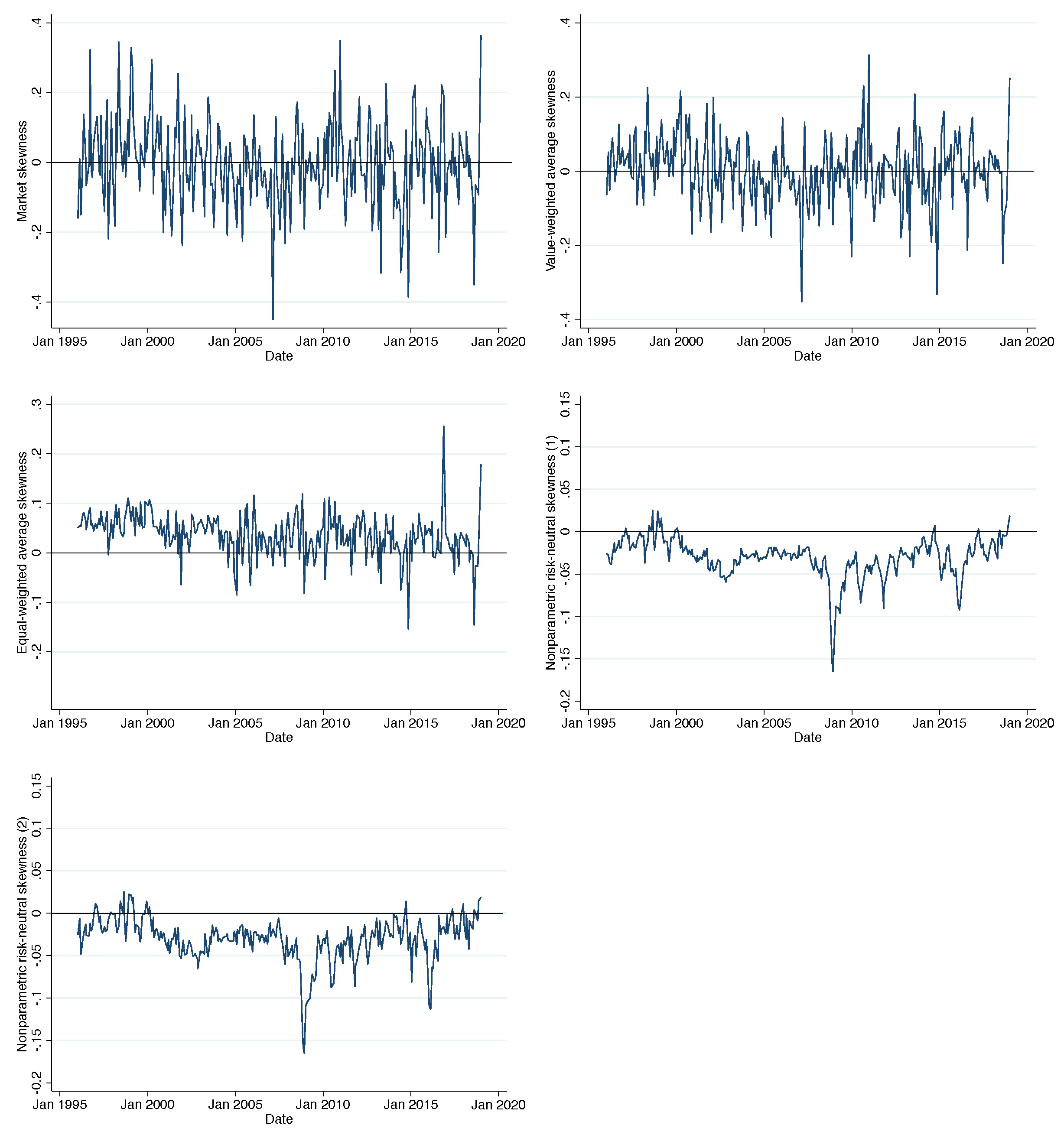
Figure 2.
Time-series movement of skewness. This figure shows the market, average realized, and nonparametric risk-neutral skewness of energy stock returns. The sample period is from January 1996 to December 2018. The nonparametric risk-neutral skewness is computed in two different ways; (1) taking the average across equal-weighted average individual skewness or (2) selecting at the end of each month the value of individual and then taking the average.

Table 1.
Summary statistics of EMI monthly return. This table shows the summary statistics of energy market index (EMI) monthly excess return over the full sample period, which is from January 1996 to December 2018. Monthly return of is the simple sum of EMI daily return, , and the correlation between and returns is as high as 98%. (See Table A1 for more details.) stands for standard deviation of .
| Year | Mean | SD | Skewness | Kurtosis | Minimum | Median | Maximum |
|---|---|---|---|---|---|---|---|
| 1996 | 0.0249 | 0.0288 | −0.8207 | 3.4403 | −0.0442 | 0.0258 | 0.0630 |
| 1997 | 0.0224 | 0.0418 | −0.1868 | 1.9234 | −0.0558 | 0.0211 | 0.0782 |
| 1998 | 0.0048 | 0.0633 | 0.2638 | 2.6285 | −0.1042 | −0.0084 | 0.1364 |
| 1999 | 0.0243 | 0.0645 | 1.1669 | 3.1001 | −0.0512 | 0.0058 | 0.1575 |
| 2000 | 0.0284 | 0.0631 | 0.3469 | 1.6690 | −0.0519 | 0.0062 | 0.1371 |
| 2001 | −0.0050 | 0.0486 | 0.7433 | 2.7513 | −0.0735 | −0.0083 | 0.1005 |
| 2002 | −0.0024 | 0.0518 | −0.5885 | 2.5463 | −0.1086 | 0.0046 | 0.0761 |
| 2003 | 0.0233 | 0.0453 | 1.1138 | 3.2004 | −0.0216 | 0.0191 | 0.1294 |
| 2004 | 0.0262 | 0.0317 | 0.4041 | 2.1495 | −0.0202 | 0.0114 | 0.0885 |
| 2005 | 0.0272 | 0.0664 | 0.2600 | 3.4421 | −0.0966 | 0.0237 | 0.1806 |
| 2006 | 0.0215 | 0.0570 | −0.0465 | 2.2568 | −0.0848 | 0.0370 | 0.1274 |
| 2007 | 0.0269 | 0.0381 | −0.0847 | 1.7228 | −0.0386 | 0.0306 | 0.0778 |
| 2008 | −0.0095 | 0.0759 | −0.3255 | 1.9853 | −0.1512 | 0.0008 | 0.1048 |
| 2009 | 0.0201 | 0.0566 | −0.9197 | 3.8556 | −0.1227 | 0.0331 | 0.1129 |
| 2010 | 0.0209 | 0.0590 | −0.5936 | 2.0549 | −0.0962 | 0.0466 | 0.0913 |
| 2011 | 0.0117 | 0.0712 | 0.2256 | 2.9588 | −0.1152 | 0.0115 | 0.1631 |
| 2012 | 0.0076 | 0.0466 | −0.9331 | 3.7565 | −0.1066 | 0.0171 | 0.0704 |
| 2013 | 0.0234 | 0.0280 | 0.1083 | 2.2029 | −0.0192 | 0.0255 | 0.0767 |
| 2014 | −0.0051 | 0.0510 | −0.4290 | 1.7975 | −0.0957 | 0.0133 | 0.0592 |
| 2015 | −0.0112 | 0.0632 | 0.8119 | 2.7141 | −0.0902 | −0.0353 | 0.1266 |
| 2016 | 0.0291 | 0.0504 | 0.5486 | 1.9749 | −0.0324 | 0.0218 | 0.1185 |
| 2017 | 0.0035 | 0.0424 | 1.0075 | 3.4931 | −0.0494 | −0.0087 | 0.1083 |
| 2018 | −0.0101 | 0.0690 | −0.5445 | 2.2442 | −0.1324 | 0.0113 | 0.1007 |
| Total | 0.0132 | 0.0561 | −0.0613 | 3.2927 | −0.1512 | 0.0131 | 0.1806 |
Table 2.
Summary statistics of energy stocks and options. This table shows the summary statistics of energy market stocks and options as well as their corresponding market capitalization over the sample period. The sample period is from January 1996 to December 2018. denotes the total number of firms available for the entire sample period.
| Energy Stocks | Energy Options | |||
|---|---|---|---|---|
| Year | No. Firms | Market Cap | No. Firms | Market Cap |
| 1996 | 273 | 423 | 90 | 395 |
| 1997 | 270 | 555 | 116 | 523 |
| 1998 | 252 | 567 | 125 | 544 |
| 1999 | 227 | 546 | 122 | 526 |
| 2000 | 196 | 611 | 104 | 568 |
| 2001 | 206 | 652 | 95 | 612 |
| 2002 | 165 | 548 | 86 | 526 |
| 2003 | 150 | 536 | 85 | 515 |
| 2004 | 151 | 712 | 99 | 692 |
| 2005 | 160 | 993 | 116 | 964 |
| 2006 | 175 | 1133 | 123 | 1093 |
| 2007 | 177 | 1334 | 119 | 1284 |
| 2008 | 172 | 1340 | 111 | 1278 |
| 2009 | 170 | 986 | 111 | 950 |
| 2010 | 163 | 1076 | 107 | 1021 |
| 2011 | 170 | 1318 | 116 | 1244 |
| 2012 | 167 | 1290 | 119 | 1214 |
| 2013 | 160 | 1449 | 122 | 1361 |
| 2014 | 159 | 1574 | 127 | 1478 |
| 2015 | 151 | 1238 | 127 | 1177 |
| 2016 | 149 | 1176 | 123 | 1124 |
| 2017 | 152 | 1249 | 125 | 1190 |
| 2018 | 142 | 1345 | 122 | 1273 |
| Total | 494 | 949 | 266 | 934 |
Table 3.
Summary statistics and correlation matrix. This table provides the summary statistics and the correlation matrix for the following variables: the energy market (EMI) excess return , energy market variance , energy market skewness , value-weighted average variance of energy stocks , equal-weighted average variance of energy stocks , value-weighted average skewness of energy stocks , and equal-weighted average skewness of energy stocks , nonparametric risk-neutral volatility of energy stocks, and , nonparametric risk-neutral skewness of energy stocks, , . and N stand for standard deviation and number of observations in our sample, respectively. The sample period is from January 1996 to December 2018.
| Panel A: Summary Statistics | |||||||||||
|---|---|---|---|---|---|---|---|---|---|---|---|
| Mean | SD | Skewness | Kurtosis | Minimum | Median | Maximum | N | ||||
| 0.0025 | 0.0132 | 0.1541 | 5.9435 | −0.0435 | 0.0018 | 0.0639 | 276 | ||||
| 0.0050 | 0.0094 | 10.7269 | 142.0966 | 0.0005 | 0.0032 | 0.1356 | 276 | ||||
| −0.0039 | 0.1231 | −0.0376 | 4.1341 | −0.4507 | −0.0071 | 0.3631 | 276 | ||||
| 0.0072 | 0.0105 | 10.1142 | 131.3646 | 0.0011 | 0.0052 | 0.1508 | 276 | ||||
| 0.0031 | 0.0903 | −0.2623 | 4.6761 | −0.3521 | 0.0051 | 0.3135 | 276 | ||||
| 0.0289 | 0.0247 | 4.3528 | 28.6839 | 0.0070 | 0.0232 | 0.2155 | 276 | ||||
| 0.0369 | 0.0441 | −0.3589 | 6.9115 | −0.1538 | 0.0420 | 0.2559 | 276 | ||||
| 0.7162 | 0.1735 | 1.6965 | 8.2693 | 0.4650 | 0.6816 | 1.6018 | 276 | ||||
| −0.0308 | 0.0239 | −1.7400 | 9.7367 | −0.1650 | −0.0283 | 0.0249 | 276 | ||||
| 0.7125 | 0.1717 | 1.7722 | 8.7897 | 0.4678 | 0.6796 | 1.6268 | 276 | ||||
| −0.0302 | 0.0264 | −1.5276 | 8.1326 | −0.1653 | −0.0272 | 0.0251 | 276 | ||||
| Panel B: Correlation Matrix | |||||||||||
| 1 | |||||||||||
| −0.0021 | 1 | ||||||||||
| 0.0413 | 0.0555 | 1 | |||||||||
| 0.0195 | 0.9306 | 0.0752 | 1 | ||||||||
| 0.0648 | 0.0575 | 0.8675 | 0.0753 | 1 | |||||||
| −0.0165 | 0.5973 | 0.0711 | 0.6383 | 0.1031 | 1 | ||||||
| −0.091 | 0.0667 | 0.6617 | 0.0803 | 0.6597 | 0.1594 | 1 | |||||
| −0.0055 | 0.6193 | 0.1045 | 0.7016 | 0.0896 | 0.6291 | 0.0671 | 1 | ||||
| −0.0298 | −0.5175 | −0.0055 | −0.4788 | −0.0234 | −0.3488 | −0.0452 | −0.5381 | 1 | |||
| −0.0076 | 0.6155 | 0.1061 | 0.6979 | 0.0923 | 0.6266 | 0.0691 | 0.9984 | −0.5371 | 1 | ||
| −0.0893 | −0.4776 | 0.0483 | −0.4363 | 0.0162 | −0.2832 | 0.0357 | −0.4777 | 0.9286 | −0.4739 | 1 | |
Table 4.
Summary statistics of control variables. This table provides the summary statistics and the correlation matrix for the following control variables. The default spread, , the term spread, . The market illiquidity measure proposed by Amihud (2002) is also included, . is a skewness between OTMP and ATMC of the energy sector options, is put-call-parity implied volatility spread variable of the energy sector options, both of which can be downloaded directly from IvyDB OptionMetrics for the sample period ranging from January 1996 to 2017. and N stand for standard deviation and number of observations in our sample, respectively.
| Panel A: Summary Statistics of Control Variables | ||||||||
|---|---|---|---|---|---|---|---|---|
| 0.0367 | 0.0091 | −0.2940 | 2.3091 | 0.0173 | 0.0379 | 0.0588 | ||
| −0.0140 | 0.0060 | −1.4891 | 6.9020 | −0.0405 | −0.0134 | −0.0011 | ||
| 0.0600 | 0.0228 | 0.3681 | 3.3019 | 0.0021 | 0.0582 | 0.1330 | ||
| 0.0023 | 0.0196 | 0.1147 | 4.2492 | −0.0676 | 0.0013 | 0.0844 | ||
| 0.0957 | 0.1170 | 3.7187 | 23.2601 | 0.0099 | 0.0593 | 1.0336 | ||
| 0.0124 | 0.0129 | 3.7522 | 26.5037 | 0.0020 | 0.0085 | 0.1273 | ||
| 0.2565 | 0.0880 | 2.6363 | 14.3155 | 0.1377 | 0.2380 | 0.8002 | ||
| 0.0410 | 0.0413 | 4.3437 | 33.3495 | 0.0001 | 0.0333 | 0.4101 | ||
| Panel B: Correlation Matrix between Control Variables | ||||||||
| 1 | ||||||||
| −0.2367 | 1 | |||||||
| −0.2810 | −0.2150 | 1 | ||||||
| 0.0592 | 0.0190 | −0.8616 | 1 | |||||
| −0.0042 | 0.0075 | −0.0245 | −0.0099 | 1 | ||||
| 0.1726 | −0.2115 | 0.0202 | 0.0322 | 0.1392 | 1 | |||
| 0.2091 | −0.5638 | 0.0453 | 0.2064 | 0.0304 | 0.3923 | 1 | ||
| 0.1454 | −0.2335 | −0.0939 | 0.2216 | 0.0202 | 0.1747 | 0.4547 | 1 | |
Table 5.
Baseline regression–Individual variables. The table contains results of the predictive regressions of the energy market excess return . and are energy market variance and skewness. and are the value-weighted average energy stock variance and skewness. and are the equal-weighted average energy stock variance and skewness. , and , are nonparametric risk-neutral volatility and skewness. p-values (two-sided) are reported using Newey–West adjusted t-statistics and in parentheses. The table also reports adjusted values. ** denotes 5% level of significance. The sample period is from January 1996 to December 2018.
| (1) | (2) | (3) | (4) | (5) | (6) | (7) | (8) | (9) | (10) | |
|---|---|---|---|---|---|---|---|---|---|---|
| Panel A: Individual Variables | ||||||||||
| 0.14 | ||||||||||
| (0.202) | ||||||||||
| 0.03 | ||||||||||
| (0.177) | ||||||||||
| 0.14 | ||||||||||
| (0.179) | ||||||||||
| 0.06 ** | ||||||||||
| (0.046) | ||||||||||
| 0.00 | ||||||||||
| (0.982) | ||||||||||
| −0.04 | ||||||||||
| (0.479) | ||||||||||
| −0.00 | ||||||||||
| (0.718) | ||||||||||
| −0.02 | ||||||||||
| (0.849) | ||||||||||
| −0.01 | ||||||||||
| (0.666) | ||||||||||
| −0.05 | ||||||||||
| (0.603) | ||||||||||
| Adj. | −0.26% | 0.20% | −0.24% | 1.11% | −0.37% | −0.18% | −0.33% | −0.35% | −0.32% | −0.26% |
| Panel B: Individual Variables with Current Market Return | ||||||||||
| −0.03 | −0.03 | −0.03 | −0.04 | −0.03 | −0.03 | −0.04 | −0.03 | −0.04 | −0.04 | |
| (0.557) | (0.488) | (0.561) | (0.383) | (0.477) | (0.518) | (0.434) | (0.473) | (0.426) | (0.460) | |
| 0.12 | ||||||||||
| (0.318) | ||||||||||
| 0.03 | ||||||||||
| (0.180) | ||||||||||
| 0.12 | ||||||||||
| (0.272) | ||||||||||
| 0.06 ** | ||||||||||
| (0.041) | ||||||||||
| −0.00 | ||||||||||
| (0.999) | ||||||||||
| −0.04 | ||||||||||
| (0.505) | ||||||||||
| −0.01 | ||||||||||
| (0.656) | ||||||||||
| −0.02 | ||||||||||
| (0.831) | ||||||||||
| −0.01 | ||||||||||
| (0.603) | ||||||||||
| −0.06 | ||||||||||
| (0.594) | ||||||||||
| Adj. | −0.56% | −0.06% | −0.53% | 0.91% | −0.63% | 0.46% | −0.57% | −0.61% | −0.55% | −0.50% |
Table 6.
Baseline regression–Combination of variables. The table contains results of the predictive regressions of the energy market excess return . and are energy market variance and skewness. and are the value-weighted average energy stock variance and skewness. and are the equal-weighted average energy stock variance and skewness. and are nonparametric risk-neutral volatility and skewness. p-values (two-sided) are reported using Newey–West adjusted t-statistics and in parentheses. The table also reports adjusted values. * and ** denote 10% and 5% level of significance, respectively. The sample periods are January 1996 to December 2018.
| (1) | (2) | (3) | (4) | (5) | |
|---|---|---|---|---|---|
| Panel A: Combination of Variables | |||||
| 0.12 | |||||
| (0.654) | |||||
| 0.03 | |||||
| (0.228) | |||||
| 0.09 | |||||
| (0.694) | |||||
| 0.06 ** | |||||
| (0.050) | |||||
| 0.01 | |||||
| (0.925) | |||||
| −0.04 | |||||
| (0.472) | |||||
| −0.01 | |||||
| (0.622) | |||||
| −0.05 | −0.06 | ||||
| (0.665) | (0.638) | ||||
| Adj. | −0.10% | 0.81% | −0.54% | −0.63% | −0.61% |
| Panel B: Combination Variables with Current Market Return | |||||
| −0.03 | −0.05 | −0.01 | −0.04 | −0.04 | |
| (0.641) | (0.415) | (0.835) | (0.551) | (0.542) | |
| 0.10 | −0.24 | 0.23 | 0.24 | 0.27 | |
| (0.718) | (0.885) | (0.534) | (0.481) | (0.443) | |
| 0.03 | −0.07 | 0.05 ** | 0.03 | 0.03 | |
| (0.227) | (0.161) | (0.042) | (0.182) | (0.175) | |
| 0.27 | |||||
| (0.854) | |||||
| 0.14 ** | |||||
| (0.034) | |||||
| −0.05 | |||||
| (0.698) | |||||
| −0.13 * | |||||
| (0.078) | |||||
| −0.02 | |||||
| (0.297) | |||||
| −0.07 | −0.07 | ||||
| (0.611) | (0.580) | ||||
| Adj. | −0.38% | 0.58% | 0.12% | −0.72% | −0.63% |
Table 7.
Comparison with economic variables. The table contains results of the predictive regressions of the energy market excess return . are the value-weighted average variance and skewness. The default spread, , the term spread, . The market illiquidity measure proposed by Amihud (2002) is also included, . is a skewness between OTMP and ATMC of the energy sector options, is put-call-parity implied volatility spread variable of the energy sector options, both of which can be downloaded directly from IvyDB OptionMetrics for the sample period ranging from January 1996 to 2017. p-values (two-sided) are reported using Newey–West adjusted t-statistics and in parentheses. The table also reports adjusted values. * and ** denote 10% and 5% level of significance, respectively. The sample period is from January 1996 to December 2018.
| (1) | (2) | (3) | (4) | |
|---|---|---|---|---|
| Business cycle and market illiquidity (1996–2018) | ||||
| −0.04 | −0.03 | |||
| (0.395) | (0.501) | |||
| 0.06 ** | 0.06 ** | 0.05 * | 0.05 * | |
| (0.036) | (0.036) | (0.076) | (0.070) | |
| −0.09 | −0.11 | −0.13 | ||
| (0.659) | (0.753) | (0.729) | ||
| 0.07 | −0.03 | −0.07 | −0.09 | |
| (0.532) | (0.909) | (0.845) | (0.809) | |
| 0.00 | 0.00 | 0.00 | 0.00 | |
| (0.976) | (0.970) | (0.989) | (0.985) | |
| −0.11 | −0.11 | |||
| (0.801) | (0.799) | |||
| 0.39 | 0.34 | |||
| (0.512) | (0.595) | |||
| Adj. | 0.41% | −0.90% | 0.69% | −0.11% |
Table 8.
Comparison with financial variables. The table contains results of the predictive regressions of the energy market excess return . and are the value-weighted average variance and skewness. The average correlation across energy stocks, , the variance risk premium of energy market stocks, , and the volatility index of energy stocks, . p-values (two-sided) are reported using Newey–West adjusted t-statistics and in parentheses. The table also reports adjusted values. ** denotes 5% level of significance.
| (1) | (2) | (3) | (4) | |
|---|---|---|---|---|
| Panel A:AC(1996–2018) | ||||
| −0.04 | ||||
| (0.422) | ||||
| 0.06 ** | 0.06 ** | 0.06 ** | ||
| (0.046) | (0.041) | (0.037) | ||
| −0.08 | −0.12 | −0.11 | ||
| (0.589) | (0.419) | (0.472) | ||
| Adj. | 1.46% | −0.69% | 0.76% | 0.12% |
| Panel B:VRP(1998–2018) | ||||
| −0.03 | ||||
| (0.549) | ||||
| 0.06 ** | 0.06 ** | 0.06 ** | ||
| (0.045) | (0.048) | (0.043) | ||
| 0.01 | 0.00 | 0.00 | ||
| (0.797) | (0.952) | (0.965) | ||
| Adj. | 1.27% | −0.40% | 0.85% | 0.52% |
| −0.03 | ||||
| (0.599) | ||||
| 0.06 ** | 0.06 ** | 0.06 ** | ||
| (0.045) | (0.048) | (0.043) | ||
| 0.01 | 0.01 | 0.01 | ||
| (0.611) | (0.698) | (0.764) | ||
| Adj. | 1.27% | −0.33% | 0.90% | 0.55% |
Publisher’s Note: MDPI stays neutral with regard to jurisdictional claims in published maps and institutional affiliations. |
© 2021 by the authors. Licensee MDPI, Basel, Switzerland. This article is an open access article distributed under the terms and conditions of the Creative Commons Attribution (CC BY) license (https://creativecommons.org/licenses/by/4.0/).
Share and Cite
MDPI and ACS Style
Yoon, J.; Ruan, X.; Zhang, J.E. The Skewness Risk in the Energy Market. J. Risk Financial Manag. 2021, 14, 620. https://0-doi-org.brum.beds.ac.uk/10.3390/jrfm14120620
AMA Style
Yoon J, Ruan X, Zhang JE. The Skewness Risk in the Energy Market. Journal of Risk and Financial Management. 2021; 14(12):620. https://0-doi-org.brum.beds.ac.uk/10.3390/jrfm14120620
Chicago/Turabian StyleYoon, Jungah, Xinfeng Ruan, and Jin E. Zhang. 2021. "The Skewness Risk in the Energy Market" Journal of Risk and Financial Management 14, no. 12: 620. https://0-doi-org.brum.beds.ac.uk/10.3390/jrfm14120620