Machine-Learning-Based Semiparametric Time Series Conditional Variance: Estimation and Forecasting

Abstract

This paper proposes a new combined semiparametric estimator of the conditional variance that takes the product of a parametric estimator and a nonparametric estimator based on machine learning. A popular kernel-based machine learning algorithm, known as the kernel-regularized least squares estimator, is used to estimate the nonparametric component. We discuss how to estimate the semiparametric estimator using real data and how to use this estimator to make forecasts for the conditional variance. Simulations are conducted to show the dominance of the proposed estimator in terms of mean squared error. An empirical application using S&P 500 daily returns is analyzed, and the semiparametric estimator effectively forecasts future volatility.

1. Introduction

It is well known that financial time series data, especially stock returns, are not predictable. On the other hand, volatility (risk) or the conditional variance of the returns is easier to predict since autocorrelations are shown to be significant in various time series data. There are a plethora of models that try and capture the dynamics of the volatility of a series, including both parametric and nonparametric models. In this paper, both a parametric and nonparametric model of the conditional variance are combined in a multiplicative way, resulting in a semiparametric estimator of the conditional variance. The semiparametric estimator is shown to dominate both fully parametric and nonparametric counterparts in forecasting ability and can successfully capture the asymmetric volatility effect of return.

To model the conditional variance of a series, one can specify a parametric model, but this can lead to misspecification issues of the volatility function. One can also specify a nonparametric model, where the explicit specification of the form of the conditional variance function is not needed. However, this may be harder to estimate when, for example, some of the conditioning set of variables are unobserved lagged conditional variances. The proposed semiparametric estimator of the conditional variance uses a parametric component as a basis. This basis is then multiplied by an adjustment factor based on the nonparametric modeling of parametric squared residuals using estimated lagged conditional variances, if present, in the conditioning set. Thus, such a semiparametric estimator combines a parametric conditional variance estimator with a nonparametric estimator of the conditional variance. The parametric component of the conditional variance is used mainly to capture the overall dynamics whereas the nonparametric part analyzes the residual variance and catches the nonlinearities in the data that the parametric component fails to capture. The generalized autoregressive conditional heteroskedasticity (GARCH) family of models are considered for the parametric estimation. For the nonparametric estimation, a popular machine learning (ML) algorithm is used, known as Kernel Regularized Least Squares (KRLS), which does not rely on linearity or additivity assumptions (Hainmueller and Hazlett 2014).

The GARCH family of models is a common method to modeling volatility as the conditional variance, ${\sigma }_t^2$, for a stocastic process $y_t$. The first among these started with Engle (1982) for the autoregressive conditional heteroskedasticity (ARCH) model and Bollerslev (1986) for the GARCH model of the conditional variance. Later, many papers following their work paved the way for other GARCH-type models that capture many stylized facts including being able to capture volatility dynamics and incorporating leverage effects (Glosten et al. (1993); Nelson (1991) and Ding et al. (1993)). All of these models are considered to be parametric and are subject to misspecification. If a GARCH model, or any other parametric model, is correctly specified, then it can be shown that the model can consistently estimate the conditional variance. However, when a parametric model is misspecified, then the volatility estimator is often inconsistent for ${\sigma }_t^2$. In this paper, we will use $ARCH\left(1\right)$ and $GARCH(1,1)$ models to estimate the parametric conditional variance and use a ML based nonparametric method to enhance the conditional variance estimates.

Nonparametric and semiparametric estimation of the conditional variance have also proven to capture dynamics in the volatility well. To estimate the conditional variance, Ziegelmann (2002) models the squared residuals, from the conditional mean equation, nonparametrically via the local exponential estimator. However, this procedure may not be applicable for the GARCH-type conditional variation. In this paper, however, the conditional variance function is considered to be semiparametric as the product of a parametric part and nonparametric part similar to Mishra et al. (2010). This framework stems from the seminal work by Glad (1998) where a multiplicative semiparametric model of the conditional mean function is formulated. In this paper, the framework is based on Glad (1998) and Mishra et al. (2010) for the conditional variance by multiplying the parametric component by the nonparametric component. However, instead of using local exponential (or polynomial) smoothing for estimating the nonparametric component as they do, we will use another nonparametric technique known as KRLS based ML.

KRLS is a common ML technique in the nonparametric ML literature. The method uses kernels to find the best fit surface in a flexible hypothesis space by minimizing a penalized least squares problem, see Hainmueller and Hazlett (2014). De Brebanter et al. (2011) refer to the same method as Least Squares Support Vector Machines (LSSVM) and propose bias corrected confidence intervals for the estimator. However, these papers study the conditional mean function, and not the conditonal variance function. This paper differs by estimating the conditional variance function with the help of ML. That is, standardized squared residuals, obtained from the conditional mean equation, are used in a ML regression to estimate the nonparametric component of the conditional variance. With the help of ML, the nonparametric component can hopefully capture the nonlinearites in the true volatility function, where the parametric component failed to do so.

Overall, this paper proposes a semiparametric estimator based on the ML technique KRLS. The proposed estimator is capable of handling in and out of sample data, where forecasting the future conditional variance based on a conditioning set is achieved. We show in simulation that the semiparametric estimator beats the parametric counterpart in terms of mean squared error. An empirical example with real data from S&P 500 daily returns is also given to illustrate the advantage of using the semiparametric ML estimator of the conditional variance, where news impact curves and out of sample forecasts are evaluated. In the empirical example, the semiparametric estimator is shown to be superior to the parametric estimators when evaluating out of sample forecasts.

The structure of this paper is as follows: Section 2 discusses the model framework of the conditional variance, Section 3 proposes the semiparametric estimator using ML to estimate the nonparametric component, Section 4 shows how forecasts are made via the semiparametric estimator, Section 5 runs through a simulation example, Section 6 illustrates an empirical example using S&P 500 daily returns, and Section 7 concludes the paper.

2. The Model

Consider the following model:

$$\begin{array}{c}{y}_t={\alpha }_t+{\epsilon }_t,\end{array}$$

(1)

$$\begin{array}{c}{\alpha }_t=g(U_t,\mathbf{\beta })\end{array}$$

(2)

where ${\epsilon }_t$ satisfies $\mathbb{E}\left[{\epsilon }_t\right|{\mathcal{F}}_{t-1}]=0$ and $\mathbb{E}\left[{\epsilon }_t^2\right|{\mathcal{F}}_{t-1}]={\sigma }_t^2$ and $U_t\in {\mathcal{F}}_{t-1}$ represents a vector of regressors, and $\mathbf{\beta }$ represents the vector of parametric parameters for the mean regression. The function $g(·)$ can be any parametric function of the data $U_t$ and parameter vector $\mathbf{\beta }$, such as an Autoregressive Moving Average (ARMA) function or a constant function for the conditional mean function. Note that since $U_t\in {\mathcal{F}}_{t-1}$, $Var\left[y_t\right|{\mathcal{F}}_{t-1}]=Var[y_t-{\alpha }_t|{\mathcal{F}}_{t-1}]=Var\left[{\epsilon }_t\right|{\mathcal{F}}_{t-1}]={\sigma }_t^2$.

Similar to Glad (1998) and Mishra et al. (2010), we can redefine the conditional variance, ${\sigma }_t^2=\mathbb{E}\left[{\epsilon }_t^2\right|{\mathcal{F}}_{t-1}]$ as

$$\mathbb{E}\left[{\epsilon }_t^2\right|{\mathcal{F}}_{t-1}]={\sigma }_{p,t}^2\mathbb{E}\left[{\left(\frac{{\epsilon }_t}{{\sigma }_{p,t}}\right)}^2|{\mathcal{F}}_{t-1}\right],$$

(3)

where ${\sigma }_{p,t}^2\in {\mathcal{F}}_{t-1}$ is found by a parametric specification of the conditional variance. Let ${\sigma }_{np,t}^2=\mathbb{E}\left[{({\epsilon }_t/{\sigma }_{p,t})}^2|{\mathcal{F}}_{t-1}\right]\in {\mathcal{F}}_{t-1}$ denote the nonparametric specification of the conditional variance. We can think of ${({\epsilon }_t/{\sigma }_{p,t})}^2$ as a new dependent variable in the nonparametric estimation stage. Then, the final semiparametric estimator of the conditional variance is

$${\sigma }_t^2={\sigma }_{p,t}^2{\sigma }_{np,t}^2.$$

(4)

The idea is that if the parametric form of the conditional variance fails to capture some feature of the true conditional variance, the nonparametric form of the conditional variance will have a multiplicative correction factor that will hopefully be easier to estimate. If the parametric conditional variance underestimates the true conditional variance, in which the parametric model will be subject to misspecification, the nonparametric component, ${\sigma }_{np,t}^2$, will be greater than one and vice versa. In the extreme case, where the parametric form of the conditional variance is correctly specified, the nonparametric component, ${\sigma }_{np,t}^2$, will hopefully be constant over time.

3. The Semiparametric ML Estimator

Since ${\epsilon }_t$ is unobservable, the first step is to obtain the residuals of the estimated regression equation.

$${\widehat{\epsilon }}_t=y_t-{\widehat{\alpha }}_t,t=1,\dots ,T$$

(5)

where ${\widehat{\alpha }}_t=\widehat{g}(U_t,\widehat{\mathbf{\beta }})$ is the estimated regression function, e.g., ARMA process and T is the total number of observations in the sample. We will then use the residuals in Equation (5) to estimate both the parametric and nonparametric components of the conditional variance.

3.1. Estimating the Parametric Component

Let ${\sigma }_{p,t}^2={\sigma }_p^2\left(X_{1,t}\right)$ denote the paramatric conditional variance, which depends on regressors $X_{1,t}\in {\mathbb{R}}^{d_1}$. We can estimate the parametric conditional variance, ${\sigma }_p^2\left(X_{1,t}\right)$, by using the squared residuals obtained from Equation (5), with any parametric form, such as an $ARCH\left(1\right)$ model, where ${\sigma }_p^2\left(X_{1,t}\right)=\omega +{\alpha }_1{\epsilon }_{t-1}^2$ and $X_{1,t}={\epsilon }_{t-1}$. Any GARCH type model may also be used, which is often estimated by the quasi maximum likelihood approach. Note that the parametric form may be misspecified. The idea is that even if the parametric form is misspecified, the nonparametric component will hopefully pick up the parts of the conditional variance that the parametric part failed to estimate correctly. Once the parametric conditional variance is estimated, predictions can be made by ${\widehat{\sigma }}_p^2\left(x_1\right)$ for some test observation $x_1$.

3.2. Estimating the Nonparametric Component via ML

To get the new dependent variable to be used in the nonparametric estimation of the conditional variance, we can estimate the standardized residuals as $z_t={\widehat{\epsilon }}_t/{\widehat{\sigma }}_p\left(X_{1,t}\right),$$t=1,\dots ,T$, using the estimated residuals and the estimated parametric conditional variance evaluated at each data point in the sample. Let $z_t^2=z^2\left(X_{2,t}\right)$ depend on regressors $X_{2,t}\in {\mathbb{R}}^{d_2}$. Note that the regressors, $X_{j,t}\in {\mathcal{F}}_{t-1}$ for $j=1,2$, are considered past information. Then, we can regress $z_t^2$ on $X_{2,t}$ to get the nonparametric component of the conditional variance.

For KRLS based ML, the function ${\sigma }_{np}^2(·)$ can be approximated by some function in the space of functions constituted by

$${\sigma }_{np}^2\left(x_2\right)=\sum _{i=1}^T{c}_t{K}_{\gamma }(X_{2,i},x_2),$$

(6)

where $X_{2,i},i=1,\dots ,T$ is the vector of regressors considered for the nonparametric estimation for some test observation $x_2$ and where $c_i,i=1,\dots ,T$ are the parameters of interest, which can be thought of as the weights of the kernel functions $K_{\gamma }(·)$. The subscript of the kernel function, $K_{\gamma }(·)$, indicates that the kernel depends on the bandwidth parameter, $\gamma$. We will use the Radial Basis Function (RBF) kernel,

$$K_{\gamma }(X_i,x_2)=e^{-\frac{1}{{\gamma }^2}\left|\right|X_i-x_2{\left|\right|}^2}.$$

(7)

Notice that the RBF kernel is very similar to the Gaussian kernel, in that it does not have the normalizing term out in front and that $\gamma$ is proportional to the bandwidth h in the Gaussian kernel often used in nonparametric local polynomial regression. This functional form is justified by a regularized least squares problem with a feature mapping function that maps x into a higher dimension, see Hainmueller and Hazlett (2014), where this derivation of KRLS is also known as Kernel Ridge Regression (KRR). Overall, KRLS uses a quadratic loss with a weighted $L_2$-regularization. Then, in matrix notation, the minimization problem is

$$\underset{\mathbf{c}}{argmin}{(\mathbf{z}-{\mathbf{K}}_{\gamma }\mathbf{c})}^{\top }(\mathbf{z}-{\mathbf{K}}_{\gamma }\mathbf{c})+\lambda {\mathbf{c}}^{\top }{\mathbf{K}}_{\gamma }\mathbf{c},$$

(8)

where $\mathbf{z}={\left(\begin{array}{ccc}{\widehat{\epsilon }}_1^2/{\widehat{\sigma }}_p^2\left(X_{1,1}\right),& \dots ,& {\widehat{\epsilon }}_T^2/{\widehat{\sigma }}_p^2\left(X_{1,T}\right)\end{array}\right)}^{\top }$ is the vector of the standardized squared residuals to be used as the responses in this regression and ${\mathbf{K}}_{\gamma }$ is the kernel matrix, with $K_{\gamma ,i,j}=K_{\gamma }(X_i,X_j)$ for $i,j=1,\dots ,T$ and $\mathbf{c}$ is the vector of coefficients that is optimized over. The solution to this minimization problem is

$$\widehat{\mathbf{c}}={({\mathbf{K}}_{\gamma }+\lambda \mathbf{I})}^{-1}\mathbf{z}.$$

(9)

The kernel function and its parameters are user specified but can be found via cross validation along with the regularization parameter $\lambda$. In simulation and in the empirical application, leave one out cross validation is used to find the hyperparameters, $\gamma$ and $\lambda$. Finally, predictions for the nonparametric ML conditional variance estimator can be made by

$${\widehat{\sigma }}_{np}^2\left(x_2\right)=\sum _{i=1}^T{\widehat{c}}_i{K}_{\gamma }(X_i,x_2),$$

(10)

for some test observation $x_2$.

3.3. The Semiparametric ML Estimator

Now that we have both the estimated parametric, ${\widehat{\sigma }}_p^2\left(x_1\right)$, and nonparametric, ${\widehat{\sigma }}_{np}^2\left(x_2\right)$, components of the conditional variance, we can estimate the final semiparametric conditional variance in a multiplicative way and predictions can be made by

$${\widehat{\sigma }}_{sp}^2\left(x\right)={\widehat{\sigma }}_p^2\left(x_1\right){\widehat{\sigma }}_{np}^2\left(x_2\right),$$

(11)

for some test observation point $x={\left(\begin{array}{cc}{x}_1^{\top },& x_2^{\top }\end{array}\right)}^{\top }$.

Notice that both $X_1$ and $X_2$ can be unobservable. To illustrate, we will discuss the $GARCH(1,1)$ model of the conditional variance, ${\sigma }_t^2\left(X_{1,t}\right)=\omega +\alpha {\epsilon }_{t-1}+{\mathbf{\beta }}_1{\sigma }_{t-1}^2$. Here, $X_{1,t}={\left(\begin{array}{cc}{\epsilon }_{t-1},& {\sigma }_{t-1}^2\end{array}\right)}^{\top }$. The estimate for ${\sigma }_{p,t}^2$ can be obtained by any parametric model based on quasi maximum likelihood estimation (QMLE), which is standard for ARCH and GARCH models. Now, suppose that we estimate the nonparametric component in a similar fashion but instead of imposing a parametric form of the conditional variance, we will use ML. That is, we estimate ${\sigma }^2\left(X_{2,t}\right)$ nonparametrically via ML, where $X_{2,t}={\left(\begin{array}{cc}{\epsilon }_{t-1},& {\sigma }_{t-1}^2\end{array}\right)}^{\top }$. In this case, we estimate the lagged residuals by Equation (5) and we will use the parametric conditional variance estimates for ${\sigma }_{t-1}^2$. Therefore, we use ${\widehat{X}}_{2,t}={\left(\begin{array}{cc}{\widehat{\epsilon }}_{t-1},& {\widehat{\sigma }}_{p,t-1}^2\end{array}\right)}^{\top }$ as regressors for the nonparametric estimation. Then, Equation (11) can be used to obtain the final conditional variance estimate. This estimator will be denoted as SPMLGARCH estimator for using a GARCH model for the parametric component and ML for the nonparametric component. Without loss of generality, the procedure can be extended to higher order lags.

4. Forecasting

To forecast the conditional variance, we can use Equations (10) and (11). Let $h\in {\mathbb{Z}}^{+}$ denote the number of periods ahead we wish to forecast, e.g., $h=1$ for a one-step-ahead forecast. First, we use the training sample to fit a parametric model of the conditional variance, ${\widehat{\sigma }}_p^2$, and forecast h periods ahead using standard techniques, ${\widehat{\sigma }}_p^2\left(x_{1,T+h}\right)$. Then, we use the standardized residuals to fit a nonparametric model of the conditional variance via ML, ${\widehat{\sigma }}_{np}^2$, and forecast h periods ahead using Equation (10), ${\widehat{\sigma }}_{np}^2\left(x_{2,T+h}\right)$. Finally combining the two components gives the h period ahead forecast for the semiparametric conditional variance,

$${\widehat{\sigma }}_{sp}^2\left(x_{T+h}\right)={\widehat{\sigma }}_p^2\left(x_{1,T+h}\right){\widehat{\sigma }}_{np}^2\left(x_{2,T+h}\right),$$

(12)

where $x_{T+h}={\left(\begin{array}{cc}{x}_{1,T+h}^{\top },& x_{2,T+h}^{\top }\end{array}\right)}^{\top }$.

In the case of the $GARCH(1,1)$ model, parametric forecasts can be made in the standard way. However, for the nonparametric case, the forecasts may depend on regressors that include future residuals and conditional variances that are unobservable. Recall that a possile vector of regressors for the nonparametric regression of ${\sigma }^2\left(X_{2,t}\right)$ can be $X_{2,t}={\left(\begin{array}{cc}{\epsilon }_{t-1},& {\sigma }_{t-1}^2\end{array}\right)}^{\top }$ as in the SPMLGARCH example discussed previously. To deal with this, we estimate future residuals, ${\epsilon }_{T+h-1}$, to be 0 for $h>1$. When $h=1$, i.e., one-step-ahead forecast, ${\epsilon }_T$ can be estimated by the T-th residual from the estimated regression function. To be consistent with the estimation procedure, the parametric conditional variance forecasts will be used for future predictions of ${\sigma }_{t-1}^2$ in $X_{2,t}$ when forecasting the nonparametric component of the conditional variance. That is, let $x_{2,T+h}={\left(\begin{array}{cc}{\widehat{\epsilon }}_{T+h-1},& {\widehat{\sigma }}_{p,T+h-1}^2\end{array}\right)}^{\top }$ denote the test observation point, or the conditioning set, to be used in forecasting the nonparametric component of the conditional variance in Equation (12).

5. Simulation

This section evaluates the semiparametric ML estimator in a simulation setting. The data-generating process will come from GJR’s model of conditional variance, which takes the leverage effect into consideration, see Glosten et al. (1993). Consider the following data-generating process (DGP):

$$\begin{array}{cc}\hfill y_t& ={\epsilon }_t\hfill \\ \hfill {\sigma }_t^2& =\omega +{\alpha }_1{\epsilon }_{t-1}^2+{\beta }_1{\sigma }_{t-1}^2+{\gamma }_1{\epsilon }_{t-1}^2\mathbf{1}({\epsilon }_{t-1}\le 0)\hfill \end{array}$$

(13)

where we assume that the mean function ${\alpha }_t=0$, $\omega =0.03$, ${\alpha }_1=0.5$, ${\beta }_1=0.4$, and ${\gamma }_1=0.03$.1 We also assume that ${\epsilon }_t={\sigma }_t{\nu }_t$, where ${\nu }_t\stackrel{i.i.d.}{\sim }N(0,1)$, $\mathbb{E}\left[{\epsilon }_t\right|{\mathcal{F}}_{t-1}]=0$, and $\mathbb{E}\left[{\epsilon }_t^2\right|{\mathcal{F}}_{t-1}]={\sigma }_t^2$. The leverage effect comes from the indicator function, $\mathbf{1}(·)$, which makes the effect of negative shocks different; a positive shock is captured by ${\alpha }_1$ and a negative shock is captured by ${\alpha }_1+{\gamma }_1$. The simulated data and GARCH models are estimated by the R package rugarch from Ghalanos (2020).2

We evaluate five models: $ARCH\left(1\right)$, see Engle (1982), denoted by ARCH, GARCH(1, 1), see Bollerslev (1986), denoted by GARCH, their semiparametric ML counterparts, denoted by SPMLARCH and SPMLGARCH, where ARCH and GARCH models are estimated in the first stage, and the fully nonparametric ML using KRLS, denoted as NPML. For NPML, the estimation procedure is similar to the procedure detailed in Section 3.2; the residuals $\left({\widehat{\epsilon }}_t\right)$, instead of the standardized residuals $\left(z_t\right)$, are used in constructing the dependent variable. For the second stage in SPMLARCH and for NPML, we let $X_{2,t}={\epsilon }_{t-1}$ and in SPMLGARCH, we let $X_{2,t}={\left(\begin{array}{cc}{\epsilon }_{t-1},& {\widehat{\sigma }}_{p,t-1}^2\end{array}\right)}^{\top }$, where ${\widehat{\sigma }}_{p,t-1}^2$ is the fitted parametric conditional variance estimates in the first stage. To avoid the starting-out effect, we discard the first 500 observations and use a sample size of $n=200$. The number of replications is $M=200$. To evaluate these five models, we will use the mean squared error (MSE) criteria.

$$MSE=\frac{1}{M}\sum _{m=1}^M\frac{1}{n-1}\sum _{t=2}^n{\left({\widehat{\sigma }}_{t,m}^2-{\sigma }_t^2\right)}^2,$$

(14)

where ${\widehat{\sigma }}_{t,m}^2$ is the estimated conditional variance at time t for replication m and ${\sigma }_t^2$ is the true condtional variance at time t. The lowest MSE suggests the best model.

Table 1. The table shows MSEs calculated by Equation (14) for the ARCH, GARCH, NPML, SPMLARCH, and SPMLGARCH models under the DGP specified in Equation (13). The sample size for each estimation is $n=200$ and the number of replications is $M=200$.

MSEs of Estimators for Conditional Variance
ARCH	GARCH	NPML	SPMLARCH	SPMLGARCH
$0.2294$	$0.0317$	$0.7982$	$0.3768$	$0.0209$

displays the MSEs for each of the five estimators considered. For this DGP, both the parametric and the semiparametric ARCH models, compared to the GARCH models, perform the worst. Although the parametric GARCH model performs adequately well, SPMLGARCH improves upon the parametric GARCH and outperforms all other models in terms of MSE. Since the ARCH models only consider lagged values of the residuals, these models fail to pick up the importance of the GARCH effects in the true conditional variance. The SPMLARCH model actually is the least preferred, comparing models with parametric estimation, and shows that the nonparametric estimation stage may not help if GARCH effects are not considered when these effects are actually present. Notice that the semiparametric estimators, SPMLARCH and SPMLGARCH, dominate the NPML estimator in terms of MSE. A possible explanation is that as long as the parametric conditional variance, estimated in the first stage, can capture some shape features of the true conditional variance function, the semiparametric estimator can outperform the fully nonparametric estimator. Regardless, the SPMLGARCH model, where GARCH effects are considered in both the parametric and nonparametric estimation stages, is deemed the most appropriate model in this scenario, which has the lowest MSE compared to the parametric GARCH model as well as compared to the others.

6. Application

In this section, we fit the semiparametric ML model to real data, obtained from Federal Reserve Economic Data (FRED).3 The data contain S&P 500 daily returns from 5 August 2016 to 5 August 2021 (1305 observations). Missing oversations due to non-trading days are imputed as means of the previous and following daily returns. We allow for the mean component ${\alpha }_t$ to be an ARMA process. For the conditional variance, we evaluate five models ARCH, GARCH, SPMLARCH, SPMLGARCH, and NPML. That is, in the first-stage parametric estimation, we estimate ${\alpha }_t$ by an ARMA model, and estimate the parametric conditional variance models $ARCH\left(1\right)$ and $GARCH(1,1)$ by using the Gaussian QMLE method. In the second-stage nonparametric modeling, we estimate ${\sigma }_{np,t}^2$ by using the conditioning set ${\epsilon }_{t-1}$ for SPMLARCH and ${\left(\begin{array}{cc}{\epsilon }_{t-1},& {\sigma }_{t-1}^2\end{array}\right)}^{\top }$ for SPMLGARCH. To evaluate out of sample predictions, we split the full sample into a training data set where $t=1,\dots ,925$ and the testing data set where $t=926,\dots ,1305$. The data are split in this way so that the volatility can be forecasted for a time period in which there is high volatility. The date $t=925$ corresponds to 20 Febuary 2020, which is right when COVID-19 started to have a huge impact on the U.S. as well as its financial markets. A rolling window scheme with the window size of $T=925$ is used for one and five steps ahead forecasts.

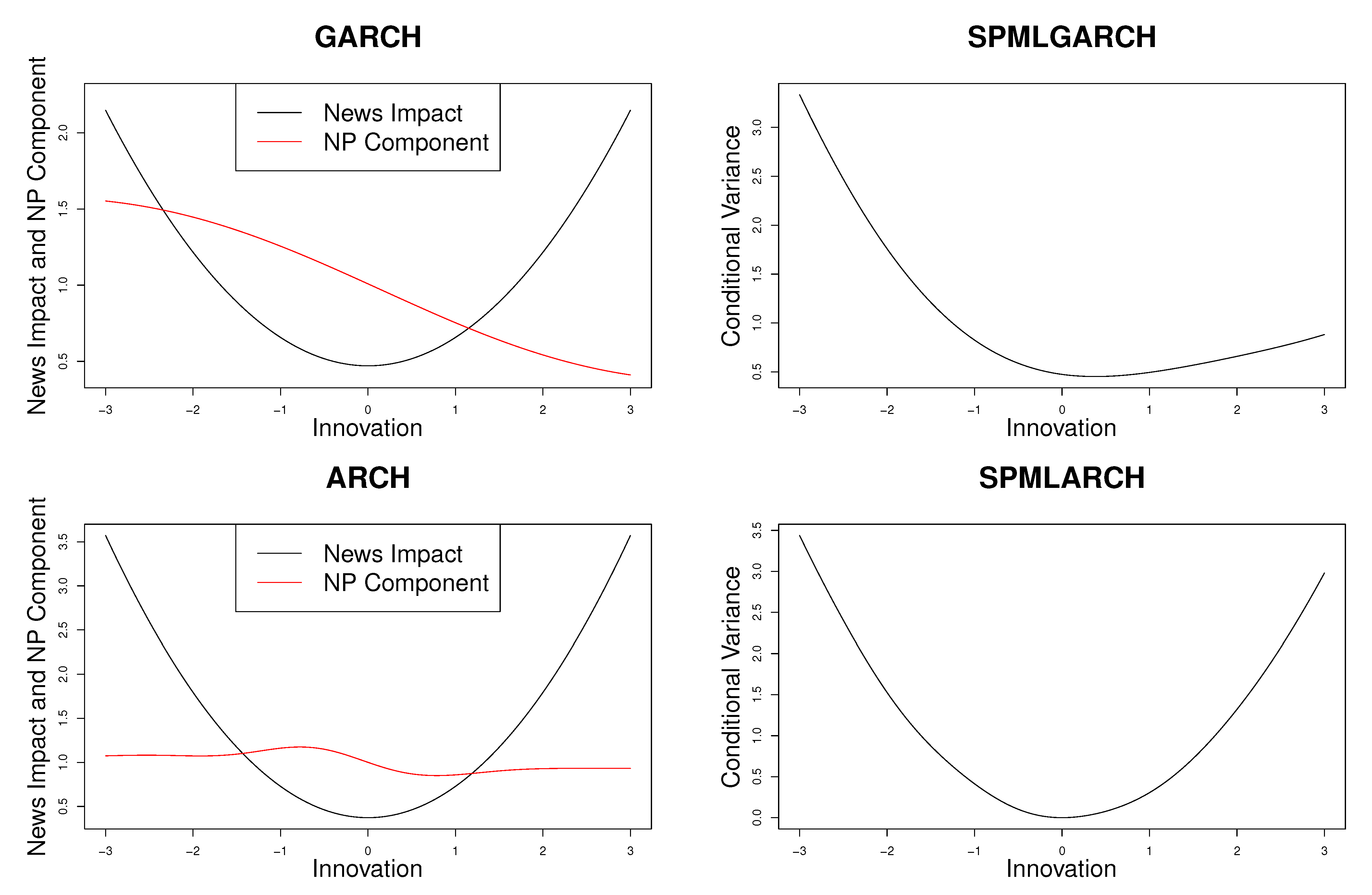
It is common practice to study the impact of the innovation, ${\epsilon }_t$ on the current conditional variance, holding all other factors fixed, which is known as the news impact curve, see Engle and Ng (1993). Due to the nature of ARCH and GARCH models, these parametric models often have symmetric news impact curves where both negative and positive shocks in absolute value have the same effect on the conditional variance, which is uncommon in financial data. The goal of estimating the nonparametric component is to pick up the asymmetry, and other nonlinearities, in the data. To see this, we can plot the nonparametric component of the conditional variance evaluated across different values of ${\epsilon }_t$. In the extreme case where the parametric model is correctly specified, the nonparametric component will be a constant and the curve will be a horizontal line at one.

Using the training data set from $t=1,\dots ,925$, the estimated news impact curve and second-stage nonlinearities are shown in the left two plots of Figure 1. Since the GARCH model has two variables in the conditioning set ${\left(\begin{array}{cc}{\epsilon }_{t-1},& {\sigma }_{t-1}^2\end{array}\right)}^{\top }$, we evaluate the curves at 100 evenly spaced points from −3 to 3 for ${\epsilon }_{t-1}$ while holding ${\sigma }_{t-1}^2={\overline{\sigma }}_p^2$ fixed at the mean of the estimated lagged parametric conditional variances. For the ARCH model, the conditioning set only contains one variable, ${\epsilon }_{t-1}$, where we evaluate the ARCH model at 100 evenly spaced points from −3 to 3. As expected, the news impact curve for both the ARCH and GARCH models seem to be symmetric. However, the nonparametric curve is not constant at one and in fact is somewhat downwards sloping. This implies that the nonparamtric component is able to detect the nonlinearity in the data and shows that the leverage effect is present in these data, which is common in various financial data.

The right two plots of Figure 1 show the conditional variance estimates for innovations spanning −3 to 3, holding other factors fixed. Visually, these plots are found by multiplying the nonparametric component and the news impact curve in the left two plots. Using Equation (11), the final conditional variance estimates do in fact show an asymmetry effect where negative shocks appear to correspond with higher conditional variances and positive shocks appear to correspond with lower conditional variances. In addition, we also estimate the semiparametric conditional variance on the entire sample using all 1305 observations, where the news impact curves are also symmetric, the nonparametric components are all downwards sloping, and the final semiparametric conditional variance estimates all exhibit the existence of the leverage effect. On the other hand, if a parametric model is estimated, the model would fail to pick up the inherent leverage effect present in the data.

To investigate the first stage estimation step,

Table 2. The table reports coefficients of the $ARCH\left(1\right)$ and $GARCH(1,1)$ models with standard errors in parentheses. The results from the top panel are based on estimates obtained from the training data set, $t=1,\dots ,925$, whereas the results from the bottom panel are based on estimates obtained from the entire data set $t=1,\dots ,1305$. ${\omega }_1$ is the intercept of the conditional variance, ${\alpha }_1$ is the coefficient of the ARCH term, and ${\beta }_1$ is the coefficient of the GARCH term. The last column contains the estimates of the mean absolute percentage change of the conditional variance due to the nonparametric component, calculated by Equation (15).

Estimated Parameters in the First Stage Estimation and Absolute Percentage Change in the Variance
	${\mathbf{\omega }}_{\mathbf{1}}$	${\mathbf{\alpha }}_{\mathbf{1}}$	${\beta }_{\mathbf{1}}$	$|\%\Delta |$Due to NP
GARCH(1, 1)	0.0382	0.1864	0.7481	12.06
	(0.0076)	(0.0328)	(0.0352)
ARCH(1)	0.3725	0.3554		9.02
	(0.0229)	(0.0611)
GARCH(1, 1)	0.0407	0.2779	0.7032	15.8
(FULL)	(0.0069)	(0.0354)	(0.0284)
ARCH(1)	0.4986	0.7443		27.53
(FULL)	(0.0296)	(0.0822)

reports the coefficients and standard errors of the $ARCH\left(1\right)$ and $GARCH(1,1)$ models. We have estimated these models based on the training data set as well as the full data set and the results are similar. A key takeaway from this table is that, the coefficient, of the GARCH term is around 0.7 and is statistically significant at the 5% level in both sample sizes, indicating that there is a GARCH effect present in the data. In addition, all ARCH effects are significant at the 5% level.

Now, to have a better understanding of how estimating the nonparametric component can help estimate the conditional variance, we evaluate the mean absolute percentage change in the semiparametric conditional variance due to the nonparametric component by the following

$$|\%{\Delta }_{np}|=\frac{1}{T-1}\sum _{t=2}^T\left|\frac{{\widehat{\sigma }}_{sp,t}^2-{\widehat{\sigma }}_{p,t}^2}{{\widehat{\sigma }}_{p,t}^2}\right|\times 100=\frac{1}{T-1}\sum _{t=2}^T\left|{\widehat{\sigma }}_{np,t}^2-1\right|\times 100.$$

(15)

The idea here is to see what percentage change is present of the semiparamtric estimate relative to the parametric estimate, and using the identity in Equation (4), this percentage change can be thought of as the amount that we need to adjust the parametric component by. The absolute percentage change is used to take into consideration that the nonparametric component may in fact increase or decrease the parametric conditional variance. These mean percentage changes are reported in the last column of Table 2. For example, the $GARCH(1,1)$ model of the conditional variance, under the sample using $t=1,\dots ,925$ observations, is on average changed by 12% via the multiplicative adjustment from the nonparametric component. The $ARCH\left(1\right)$ model is on average affected by a 9% change. Furthermore, in the full sample these estimates are even larger, indicating that the estimation of the nonparametric component is vital in picking up nonlinearities or other signals from the conditional variance that the parametric models failed to pick up. Lastly, the estimate for the $ARCH\left(1\right)$ model is the largest at around 28%. A possible explanation is that, under the full sample, which includes the highly volatile time period due to COVID-19, the parametric ARCH model may fail to pick up the these highly volatile peaks in the data, so the nonparametric part may have to uncover more of the signal from the data, and as a result the parametric component may change drastically.

Now, to evaluate forecasts, the validation set is used with a rolling window scheme. A window width of 925 observations is used to re-estimate a model and to forecast $h=1$ and $h=5$ periods ahead. First, we train a model, both parametric and nonparametric components, from the first 925 observations and forecast h periods ahead. For the nonparametric component, the hyperparameters, $\gamma$ and $\lambda$, are found via leave one out cross validation (LOOCV). Then, we roll the window h periods forward and re-estimate the parametric component using the new data set. For the nonparametric component, $\widehat{\mathbf{c}}$ is re-estimated using the new data; however, instead of performing cross validation repeatedly to estimate the hyperparameters, $\gamma$ and $\lambda$, these hyperparameters will be the ones found in the original sample using $t=1,\dots ,925$ observations, i.e., observations in the first window.

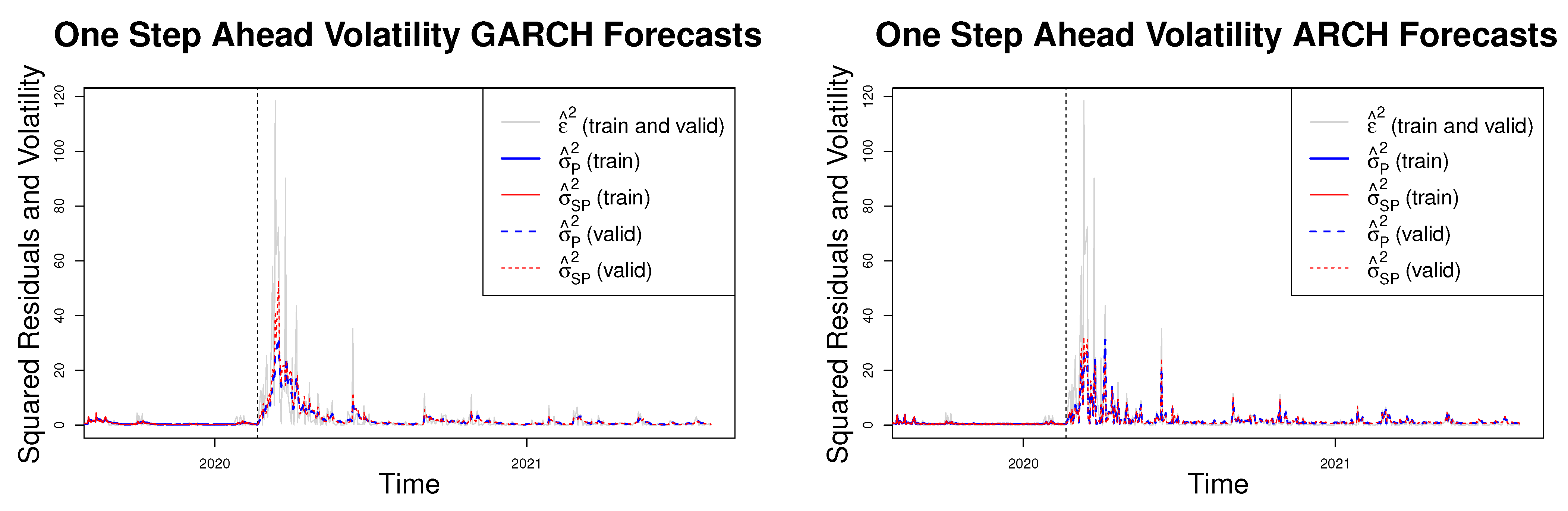
The one-step-ahead, $h=1$, forecasts are plotted in Figure 2. The left plot contains the GARCH and SPMLGARCH forecasts and the right plot contains the ARCH and SPMLARCH forecasts. Note that the last 506 observations are plotted to save space in the figures but the rolling window procedure uses the entire sample of 1305 observations. Since the true conditional variance is unknown we will use the squared residuals as a proxy. In order to do so, we estimate a parametric model, e.g., ARMA process, of the mean and obtain the residuals for the entire sample using Equation (5) and square them as an estimate of the conditional variance.4 This will be used for reference when comparing the conditional variance estimates obtained from the five models.

As we can see from the data, the conditional variance is very high during March of 2020, depicted by the grey curves indicating the squared residuals. The red and blue curves indicate the semiparametric and parametric estimates of the conditional variance. All four models appear to pick up the peaks of the conditional variances especially around March of 2020, the most volatile period of the series. However, looking closely at the figures, both SPMLGARCH and SPMLARCH pick up more of the volatility peaks around this time, indicating that the semiparametric ML models may be better suited for forecasting the volatility of S&P 500 returns.

As mentioned previously, the true conditional variance is unknown, and as a proxy we will use the squared residuals estimated from an ARMA process of the entire sample. For this data set, we found ${\alpha }_t$ to follow an $MA\left(2\right)$, under the full sample. To assess forecasting ability, we will use the root-mean-squared forecast error (RMSFE) as

$$RMSFE=\sqrt{\frac{1}{T^{\prime }}{\sum }_{t=1}^{T^{\prime }}{({\widehat{\sigma }}_t^2-{\widehat{{\epsilon }_t}}^2)}^2}$$

(16)

where ${\widehat{\epsilon }}_t$ are the estimated residuals under the full sample.

Table 3. The table reports RMSFE’s for $h=1$ and $h=5$ steps ahead forecasts and for the following estimators: SPMLGARCH, SPMLARCH, GARCH, ARCH, and NPML.

RMSFE’s of Estimators for Forecasting Conditional Variance
	SPMLGARCH	GARCH	SPMLARCH	ARCH	NPML
One Step Ahead	$8.5628$	$8.7587$	$9.6357$	$9.6594$	$10.4932$
Five Steps Ahead	$8.9648$	$9.0916$	$10.0129$	$10.0471$	$10.5647$

reports the RMSFE’s of the one and five steps ahead forecasts. For both $h=1$ and $h=5$, SPMLGARCH outperforms all other models in terms of having the lowest MSFE. In addition both the parametric and semiparametric GARCH models outperform the ARCH models, implying that GARCH effects may be present in the data, as we have seen from Table 2. In both ARCH and GARCH cases, the semiparametric counterparts perform better than the parametric ones. In addition, both semiparametric estimators exhibit superior foecasting ability relative to the nonparametric estimator, implying that the parametric components play a role in detecting some features of the true volatility function. Overall, SPMLGARCH appears to be the best model for forecasting the volatility of S&P 500 daily returns.

7. Conclusions

This paper proposes a semiparametric estimator for the conditional variance of a stochastic series. The estimator combines a parametric component and a nonparametric component via ML in a multiplicative way. The estimator is able to pick up asymmetric effects even when the parametric component can not. The ability to find asymmetric effects is directly due to the nonparametric ML estimation stage, where nonlinearities can be estimated via a kernel-based machine learning algorithm. A metric is also created to show the importance of the nonparametric component by providing on average how much the parametric component is changed by. We show that the semiparametric estimator performs better in simulations, and in the empirical application, the proposed estimator is superior to the other considered models and is able to forecast future volatility given a conditioning set.

References

- Bollerslev, Tim. 1986. Generalized Autoregressive Conditional Heteroskedasticity. Journal of Econometrics 31: 307–27. [Google Scholar] [CrossRef] [Green Version]
- Borchers, Hans W. 2021. Pracma: Practical Numerical Math Functions, R Package Version 2.3.3; Available online: https://cran.r-project.org/web/packages/pracma/index.html (accessed on 5 August 2021).
- De Brabanter, Kris, Jos De Brabanter, Johan A. K. Suykens, and Bart De Moor. 2011. Approximate Confidence and Prediction Intervals for Least Squares Support Vector Regression. IEEE Transactions on Neural Networks 22: 110–20. [Google Scholar] [CrossRef] [PubMed]
- Ding, Zhuanxin, Clive W. J. Granger, and Robert F. Engle. 1993. A Long Memory Property of Stock Market Returns and a New Model. Journal of Empirical Finance 1: 83–106. [Google Scholar] [CrossRef]
- Engle, Robert F. 1982. Autoregressive Conditional Heteroskedasticity with Estimates of the Variance of UK Inflation. Econometrica 50: 987–1008. [Google Scholar] [CrossRef]
- Engle, Robert F., and Victor K. Ng. 1993. Measuring and Testing the Impact of News on Volatility. The Journal of Finance 48: 1749–78. [Google Scholar] [CrossRef]
- Ghalanos, Alexios. 2020. Rugarch: Univariate GARCH Models, R Package Version 1.4-4; Available online: https://cran.r-project.org/web/packages/rugarch/index.html (accessed on 5 August 2021).
- Glad, Ingrid K. 1998. Parametrically Guided Non-parametric Regression. Scandinavian Journal of Statistics 25: 649–68. [Google Scholar] [CrossRef]
- Glosten, Lawrence R., Ravi Jagannathan, and David E. Runkle. 1993. On the Relationship Between the Expected Value and the Volatility of the Nominal Excess Return on Stocks. The Journal of Finance 48: 1779–801. [Google Scholar] [CrossRef]
- Hainmueller, Jens, and Chad Hazlett. 2014. Kernel Regularized Least Squares: Reducing Misspecification Bias with a Flexible and Interpretable Machine Learning Approach. Political Analysis 22: 143–68. [Google Scholar] [CrossRef]
- Hyndman, Rob J., George Athanasopoulos, Christoph Bergmeir, Gabriel Caceres, Leanne Chhay, Mitchell O’Hara-Wild, Fotios Petropoulos, Slava Razbash, Earo Wang, and Farah Yasmeen. 2020. Forecast: Forecasting Functions for Time Series and Linear Models, R Package Version 8.13; Available online: https://cran.r-project.org/web/packages/forecast/index.html (accessed on 5 August 2021).
- Mishra, Santosh, Liangjun Su, and Aman Ullah. 2010. Semiparametric Estimator of Time Series Conditional Variance. Journal of Business & Economic Statistics 28: 256–74, Research Collection School Of Economics. [Google Scholar]
- Nelson, Daniel B. 1991. Conditional Heteroskedasticity in Asset Returns: A New Approach. Econometrica 59: 347–70. [Google Scholar] [CrossRef]
- Warnes, Gregory R., Ben Bolker, Gregor Gorjanc, Gabor Grothendieck, Ales Korosec, Thomas Lumley, Don MacQueen, Arni Magnusson, and Jim Rogers. 2017. gdata: Various R Programming Tools for Data Manipulation, R package Version 2.18.0; Available online: https://cran.r-project.org/web/packages/gdata/index.html (accessed on 5 August 2021).
- Wickham, Hadley, Romain François, Lionel Henry, and Kirill Müller. 2021. dplyr: A Grammar of Data Manipulation, R Package Version 1.0.7; Available online: https://cran.r-project.org/web/packages/dplyr/index.html (accessed on 5 August 2021).
- Zeileis, Achim, and Gabor Grothendieck. 2005. zoo: S3 Infrastructure for Regular and Irregular Time Series. Journal of Statistical Software 14: 1–27. [Google Scholar] [CrossRef] [Green Version]
- Ziegelmann, Flavio A. 2002. Nonparametric Estimation of Volatility Functions: The Local Exponential Estimator. Econometric Theory 18: 985–91. [Google Scholar] [CrossRef]
Figure 1.
The left two plots show the news impact curves in black and second-stage nonlinearities in red for S&P 500 daily returns. The right two plots show the conditional variance estimates for SPMLGARCH and SPMLGARCH.
Figure 2.
The left plot shows the one-step-ahead GARCH and SPMLGARCH forecasts and the right plot shows the one-step-ahead ARCH and SPMLARCH forecast. The forecast period is from , or 21 Febuary 2021 to 5 August 2021. The vertical black dashed line indicates the start of the forecasting period. The red and blue curves indicate the semiparametric and parametric models, respectively. The solid curves represent fitted values of the conditional variance based on the training data set and the dashed curves denote the forecasts based on the validation data set. The forecasts were calculated using a rolling window scheme of window size 925.