Discrete-Time Takagi-Sugeno Stabilization Approach Applied in Autonomous Vehicles

Abstract

This paper deals with a new robust control design for autonomous vehicles. The goal is to perform lane-keeping under various constraints, mainly unknown curvature and lateral wind force. To reach this goal, a new formulation of Parallel Distributed Compensation (PDC) law is given. The quadratic Lyapunov stability and stabilization conditions of the discrete-time Takagi–Sugeno (T-S) model representing the autonomous vehicles are discussed. Sufficient design conditions expressed in terms of strict Linear Matrix Inequalities (LMIs) extracted from the linearization of the Bilinear Matrix Inequalities (BMIs) are proposed. An illustrative example is provided to show the effectiveness of the proposed approach.

1. Introduction

Autonomous vehicles require sensors to collect information about the road and a central processing unit to analyze all the data for making decisions appropriately. The sensors needed will include LIDARs, radars, cameras, GPS and ultrasound [1]; these sensors will be used to recognize the vehicles’ surroundings and measure the distance between the vehicle and nearby objects so the central processing unit can evaluate them and respond accordingly. Since some of these sensors are very expensive e.g., the sideslip angel at the center of gravity or/lateral velocity are crucial for vehicle stability, thus playing a key role in lateral control. However, in practice these variables can be only measured with very expensive sensors. Then, we should design an observer to estimate them. We also used output feedback control to avoid using such expensive sensors for control implementation. ${\mathsf{\vartheta }}_{\mathrm{y}}={\mathsf{\vartheta }}_{\mathrm{x}}\mathsf{\beta }$. Where ${\mathsf{\vartheta }}_{\mathrm{y}}$ is the lateral velocity ${\mathsf{\vartheta }}_{\mathrm{x}}$ is the vehicle speed and $\mathsf{\beta }$ is the sideslip angle.

In recent years, lateral control of autonomous vehicles has attracted great attention from academic [2] and industrial communities [3,4] and many results have been reported [5,6,7]. Some authors suggest new lateral control system architecture by combining the fuzzy logic and PID control [8]. Others focused on stabilizing lateral dynamics with considerations of parameters uncertainties and control saturation through robust yaw control. A robust yaw-moment controller design for improving vehicle handling and stability with consideration of parameters uncertainties and control saturation has been developed [9]. However, the state vector contains only two parameters to be controlled, which are the yaw rate and the sideslip angle; in this case, there is not enough information about the state of the vehicles that allows for their control in a tight way.

Sun et al. [10] present a non-model-based controller for vehicle dynamics systems to improve lateral stability, where output tracking control and adaptive dynamic programing approaches are employed to track the desired yaw rate and, at the same time, mitigate the sideslip angle, roll angle, and roll rate of the vehicle.

Considering Sun et al. [10], the proposed idea does not have a mathematical model, which means there are no mathematical stability and stabilization conditions to get access to the system control.

On the other hand, some authors investigated vision-based autonomous driving with deep learning and reinforcement learning methods. Different from the end-to-end learning method, this method breaks the vision-based lateral control system down into a perception module and a control module [11]. Nonetheless, there are no constraints in the model, e.g., lateral wind force applied to the vehicles, unknown road curvature and steering physical saturation. This implies that the introduced method is still far from real-world driving situations. For instance, an asymptotic stabilization problem for a class of nonlinear under-actuated systems was studied by Jiang and Astolfi [12]. Its solution, together with the back stepping and the forward control design methods, is exploited in the control of the nonlinear lateral dynamics of a vehicle. This technique proved that with the established controller, a vehicle is able to track any feasible reference at a constant speed and the lateral deviation converges to zero.

The issues in this case are there is a constant longitudinal vehicle speed, only one intern variable that can be controlled and the stability is local.

The lateral control of an autonomous and connected vehicle (ACV), especially in emergencies, is important from a safety point of view. The trajectory to be followed by an ACV must either be planned in real-time or communicated from its preceding vehicle, which was introduced by Liu et al. [13]; yet, this technique has a constant longitudinal velocity and no internal variables.

Zhang and Wang [14] investigated the combined active front wheel steering/direct yaw moment control for the improvement of a vehicle lateral stability and vehicle handling performance. The authors’ more particular assumption [14] is that the longitudinal velocity is not constant, but it varies within a range. Both the nonlinear tyre model and the variation of the longitudinal velocity are considered in vehicle system modeling. To track the system reference, a generalized proportional-integral (PI) control law is proposed. There is still the problem of no constraints on the model. Besides, robust non-linear control was discussed. It uses barrier Lyapunov function under lateral offset called deviation error as a constraint for the lateral control of autonomous vehicles [15,16]. Nevertheless, there is only one intern variable on the state vector that can be controlled, there are no constraints and no sweeping into longitudinal velocity. In addition, only partial state information is available for real-time control implementation.

All the above lateral control methods do not use an observer to compute the entire vehicle state vector to ensure an efficient and accurate control scheme. The first motivation came from the above issues in lateral control of autonomous vehicles. Based on the above discussion, the T-S fuzzy control method is further investigated. The T-S fuzzy control gives the possibility to sweep in large vehicles’ speed variation range. Furthermore, this feature helps to improve the closed loop performance of the autonomous vehicles under different constraints. The T-S fuzzy control systems are efficient and successful because they can describe nonlinear systems in a convex form with local and simple consequents. However, the T-S fuzzy systems control approach belongs to the state feedback control; that is, they require the entire system state to be available. Getting more information about the vehicle states indeed is of paramount importance for efficient control.

Some methods are developed for the vector state estimation. We cite Tong et al. [17]’s work, where a novel observer based adaptive fuzzy output-feedback back stepping control is designed; thus, the unmeasurable states are estimated based on the designed fuzzy state observer. Moreover, a novel integral sliding mode control is designed for the T-S fuzzy model based on Semi Markovian Jump System with immeasurable premise variables [18]. Other methods are developed to improve the control and the stabilization technique [19]. The authors proposed a new mathematical model, where the state equation is expressed by a class of nonlinear stochastic differential equations with parameter uncertainties. The uncertainties appear in the controller and the system coefficients. The idea is to solve the problems as solving the non-fragile robust stochastic stabilization and non-fragile robust ${\mathrm{H}}_{\infty }$ control via LMIs. The authors of [20] proposed a novel ${\mathrm{H}}_2/{\mathrm{H}}_{\infty }$ control scheme with Markovian Jump, advanced parameter estimation techniques are integrated into the proposed method to achieve an accurate model and better control performance.

Recently, several studies have focused on steering system control, especially fuzzy control systems [5,6,7]. These authors achieved very interesting results regarding lateral control based on Takagi–Sugeno models. Various constraints such as road with unknown curvature, steering saturation and lateral wind force, sweeping into large range of vehicle longitudinal speed and exploiting an approximated vector state containing six intern variables for effective control were fully used in their work. However, the authors used a non-quadratic Lyapunov function to reduce the conservatism caused by the use of common quadratic Lyapunov functions. On the other hand, the proposed non-quadratic Lyapunov function is complicated and complex in implementation, which results in more complexity of the system. Nevertheless, even when a nonquadratic Lyapunov is used for the T-S control scheme combined with the PDC control law, for example, the solution is a set of bilinear matrix inequalities. In addition, conservatism will always exist. Due to this complexity, the authors were forced to use approximations and assumptions for the control purpose.

Using assumptions and approximations in the automatic control signifies that there are still problems in the model, and it needs more improvements to represent the desired system dynamics.

The second and main motivation is based on the lacks introduced by Nguyen et al. [5], Nguyen et al. [6], and Sentouh et al. [7]. This work is based on the following summarized contributions:

(1)

A Quadratic Lyapunov function is considered to simplify the implementation of the system, to minimize the system complexity and to create the ellipsoid convex form.

(2)

An Improved PDC controller is designed. We introduce a new mathematical term in the classic PDC control law; this term is composed of the optimized gains times the gradient term of the state vector. This is to make the trajectory slides faster to the global minimum of the ellipsoid shape created by the Lyapunov function applied to the T-S system. This improved PDC controller ensures relaxed results even when we use the quadratic energy Lyapunov function.

(3)

Contrary to Nguyen et al. [5], Nguyen et al. [6], and Sentouh et al. [7] and others in the first motivation mentioned, the state vector will not be approximated. It will be measured, and it contains six real state variables values using Luenberger multiobservers.

(4)

First time application of Jemmali et al. [21]’s technique for the autonomous vehicles.

The paper is summarized as follows. The second section presents vehicle modeling. The third section presents the control design for discrete-time T-S systems, which focuses on the stabilization of discrete-time T-S fuzzy system based on the new PDC control law and the synthesis of multi-observers. The fourth section is devoted to application in steering control. Finally, the last section presents the new results and compares them with previous results.

2. Vehicle Modeling

This section presents the different steps used for vehicle modeling. First, the vehicle parameters are introduced and presented in

Table 1. Definition of parameters.

Parameters	Description	Value
${\mathrm{B}}_{\mathrm{s}}$	Steering system damping	5.73
${\mathrm{C}}_{\mathrm{f}}$	Front cornering stiffness	57,000 N/rad
${\mathrm{C}}_{\mathrm{r}}$	Rear cornering stiffness	59,000 N/rad
${\mathrm{I}}_{\mathrm{s}}$	Steering system moment of inertia	0.02 kg·m2
${\mathrm{I}}_{\mathrm{z}}$	Vehicle yaw moment of inertia	2800 kg·m2
${\mathrm{K}}_{\mathrm{p}}$	Manual steering column coefficient	0.5
${\mathrm{l}}_{\mathrm{f}}$	Distance from the CG to the front axle	1.3 m
${\mathrm{l}}_{\mathrm{r}}$	Distance from the CG to the rear axle	1.6 m
${\mathrm{l}}_{\mathrm{s}}$	Look-ahead distance	5 m
${\mathrm{l}}_{\mathrm{w}}$	Distance from the CG to the impact center of the wind force	0.4 m
$\mathrm{M}$	Mass of the vehicle	2025 kg
${\mathrm{R}}_{\mathrm{s}}$	Steering gear ratio	16
${\mathsf{\sigma }}_{\mathrm{t}}$	Tyre length contact	0.13 m

.

2.1. Lateral Dynamics Model of the Vehicle

Extracting from the well-known bicycle model presented by Rajamani [22], the obtained model of the vehicle lateral dynamics is expressed as:

$$\left[\begin{array}{c}\dot{\mathsf{\beta }}\\ \dot{\mathrm{r}}\end{array}\right]=\left[\begin{array}{cc}{\mathrm{a}}_{11}& {\mathrm{a}}_{12}\\ {\mathrm{a}}_{21}& {\mathrm{a}}_{22}\end{array}\right]\left[\begin{array}{c}\mathsf{\beta }\\ \mathrm{r}\end{array}\right]\mathsf{\delta }+\left[\begin{array}{c}{\mathrm{e}}_1\\ {\mathrm{e}}_2\end{array}\right]{\mathrm{f}}_{\mathrm{w}},$$

(1)

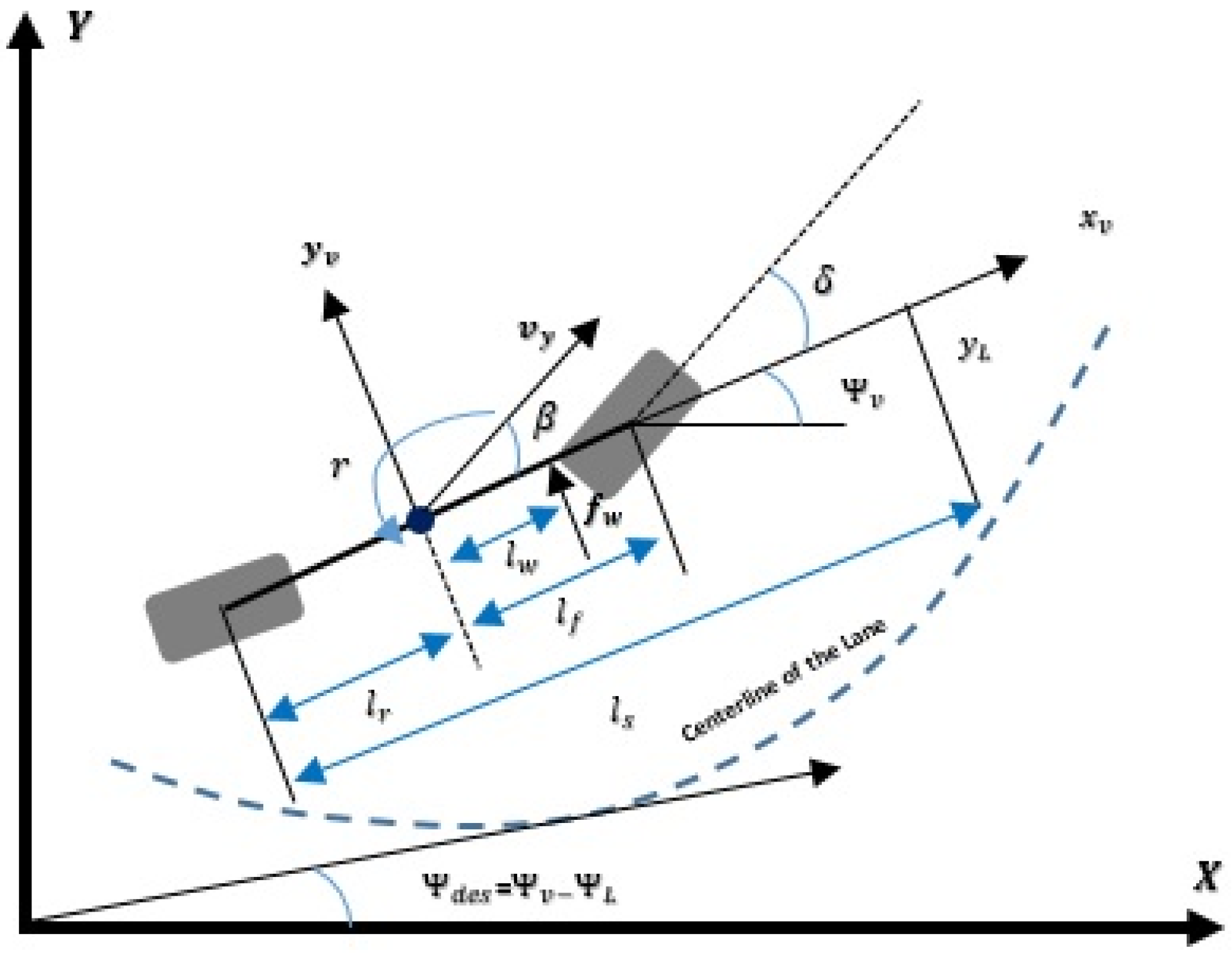
where β is the sideslip angle at the center of gravity (CG), and the yaw rate is r shown in Figure 1. As represented in Equation (1), ${\mathrm{f}}_{\mathrm{w}}$ is the lateral wind force, and the system matrices elements are written as follows:

$$\begin{gathered} {\mathrm{a}}_{11}=-2\frac{\left({\mathrm{C}}_{\mathrm{r}}+{\mathrm{C}}_{\mathrm{f}}\right)}{\mathrm{m}{\mathsf{\vartheta }}_{\mathrm{x}}};{\mathrm{a}}_{12}=2\frac{\left({\mathrm{l}}_{\mathrm{r}}{\mathrm{C}}_{\mathrm{r}}-{\mathrm{l}}_{\mathrm{f}}{\mathrm{C}}_{\mathrm{f}}\right)}{\mathrm{m}{\mathsf{\vartheta }}_{\mathrm{x}}^2}-1; \\ {\mathrm{a}}_{21}=2\frac{\left({\mathrm{l}}_{\mathrm{r}}{\mathrm{C}}_{\mathrm{r}}-{\mathrm{l}}_{\mathrm{f}}{\mathrm{C}}_{\mathrm{f}}\right)}{{\mathrm{I}}_{\mathrm{z}}};{\mathrm{a}}_{22}=-2\frac{\left({\mathrm{l}}_{\mathrm{r}}^2{\mathrm{C}}_{\mathrm{r}}^2+{\mathrm{l}}_{\mathrm{r}}^2{\mathrm{C}}_{\mathrm{f}}\right)}{{\mathrm{I}}_{\mathrm{z}}{\mathsf{\vartheta }}_{\mathrm{x}}}. \\ {\mathrm{b}}_1=\frac{2{\mathrm{C}}_{\mathrm{f}}}{\mathrm{m}{\mathsf{\vartheta }}_{\mathrm{x}}};{\mathrm{b}}_2=\frac{2{\mathrm{l}}_{\mathrm{f}}{\mathrm{C}}_{\mathrm{f}}}{{\mathrm{I}}_{\mathrm{z}}};{\mathrm{e}}_1=\frac{1}{\mathrm{m}{\mathsf{\vartheta }}_{\mathrm{x}}};{\mathrm{e}}_2=\frac{{\mathrm{l}}_{\mathrm{w}}}{{\mathrm{I}}_{\mathrm{z}}}. \end{gathered}$$

2.2. Road-Vehicle Positioning

The vehicle positioning dynamics on the road is described by [22]:

$$\{\begin{array}{c}{\dot{\mathrm{y}}}_{\mathrm{L}}={\mathsf{\vartheta }}_{\mathrm{x}}\mathsf{\beta }+{\dot{\mathrm{l}}}_{\mathrm{s}}\mathrm{r}+{\mathsf{\vartheta }}_{\mathrm{x}}{\mathsf{\psi }}_{\mathrm{L}}.\\ {\dot{\mathsf{\psi }}}_{\mathrm{L}}=\mathrm{r}-{\mathsf{\vartheta }}_{\mathrm{x}}{\mathsf{\rho }}_{\mathrm{r}}.\end{array}$$

(2)

where y_L is the lateral deviation error from the centerline of the lane projected forward a look- ahead distance, ${\mathrm{l}}_{\mathrm{s}}$ and ${\mathsf{\psi }}_{\mathrm{L}}$ are the heading error between the tangent to the road and the vehicle orientation. The road curvature is indicated by ${\mathsf{\rho }}_{\mathrm{r}}$.

2.3. Steering System Model

The electronic power steering is given as follows [23]:

$$\ddot{\mathsf{\delta }}=2\frac{{\mathrm{K}}_{\mathrm{p}}{\mathrm{C}}_{\mathrm{f}}{\mathsf{\sigma }}_{\mathrm{t}}}{{\mathrm{R}}_{\mathrm{s}}^2{\mathrm{I}}_{\mathrm{s}}}\mathsf{\beta }+2\frac{{\mathrm{K}}_{\mathrm{p}}{\mathrm{C}}_{\mathrm{f}}{\mathsf{\sigma }}_{\mathrm{t}}}{{\mathrm{R}}_{\mathrm{s}}^2{\mathrm{I}}_{\mathrm{s}}}\frac{{\mathrm{l}}_{\mathrm{f}}}{{\mathsf{\vartheta }}_{\mathrm{x}}}\mathrm{r}\cdots -2\frac{{\mathrm{K}}_{\mathrm{p}}{\mathrm{C}}_{\mathrm{f}}{\mathsf{\sigma }}_{\mathrm{t}}}{{\mathrm{R}}_{\mathrm{s}}^2{\mathrm{I}}_{\mathrm{s}}}\mathsf{\delta }-\frac{{\mathrm{B}}_{\mathrm{s}}}{{\mathrm{I}}_{\mathrm{s}}}\dot{\mathsf{\delta }}+\frac{1}{{\mathrm{R}}_{\mathrm{s}}{\mathrm{I}}_{\mathrm{s}}}{\mathrm{T}}_{\mathrm{s}}.$$

(3)

where ${\mathrm{T}}_{\mathrm{s}}$ is the steering torque, δ is the steering angle, l_s is the inertia moment of the steering column, B_s is the damping factor of the column, ${\mathrm{R}}_{\mathrm{s}}$ is the reduction ratio of the column, ${\mathsf{\sigma }}_{\mathrm{t}}$ is the width of the tyre contact finally, the manual steering column coefficient is ${\mathrm{K}}_{\mathrm{p}}$.

2.4. Vehicle Control-Based Model

From the previous models (1), (2) and (3), the road-vehicle continuous-time model utilized for the aim of system control is written as follows:

$$\dot{\mathrm{x}}\left(\mathrm{t}\right)={\mathrm{A}}_{\mathrm{c}}\mathrm{x}\left(\mathrm{t}\right)+{\mathrm{B}}_{\mathrm{c}}\mathrm{u}\left(\mathrm{t}\right)+{\mathrm{B}}_{\mathrm{cw}}\mathrm{w}\left(\mathrm{t}\right).$$

(4)

where

• $\mathrm{x}={\left[{\mathsf{\beta }\mathrm{r}\mathsf{\psi }}_{\mathrm{L}}{\mathrm{y}}_{\mathrm{L}}\mathsf{\delta }\dot{\mathsf{\delta }}\right]}^{\mathrm{T}}$ is the vehicle vector state,
• $\mathrm{w}={\left[{\mathrm{f}}_{\mathrm{w}}{\mathsf{\rho }}_{\mathrm{r}}\right]}^{\mathrm{T}}$ is the disturbance vector,
• and $\mathrm{u}={\mathrm{T}}_{\mathrm{s}}$ is the input vector.

The control-based system matrices in (4) are expressed as:

$${\mathrm{A}}_{\mathrm{c}}=\left[\begin{array}{cc}\begin{array}{ccc}{\mathrm{a}}_{11}& {\mathrm{a}}_{12}& 0\\ {\mathrm{a}}_{21}& {\mathrm{a}}_{22}& 0\\ 0& 1& 0\end{array}& \begin{array}{ccc}0& {\mathrm{b}}_1& 0\\ 0& {\mathrm{b}}_2& 0\\ 0& 0& 0\end{array}\\ \begin{array}{ccc}{\mathrm{v}}_{\mathrm{x}}& {\mathrm{l}}_{\mathrm{s}}& {\mathrm{v}}_{\mathrm{x}}\\ 0& 0& 0\\ {\mathrm{a}}_{61}& {\mathrm{a}}_{62}& 0\end{array}& \begin{array}{ccc}0& 0& 0\\ 0& 0& 1\\ 0& {\mathrm{a}}_{65}& {\mathrm{a}}_{66}\end{array}\end{array}\right];{\mathrm{B}}_{\mathrm{cw}}=\left[\begin{array}{c}\begin{array}{cc}{\mathrm{e}}_1& 0\\ {\mathrm{e}}_2& 0\\ 0& -{\mathrm{v}}_{\mathrm{x}}\end{array}\\ \begin{array}{cc}0& 0\\ 0& 0\\ 0& 0\end{array}\end{array}\right];{\mathrm{B}}_{\mathrm{c}}=\left[\begin{array}{c}\begin{array}{c}0\\ 0\end{array}\\ 0\\ \begin{array}{c}0\\ 0\\ \frac{1}{{\mathrm{R}}_{\mathrm{s}}{\mathrm{I}}_{\mathrm{s}}}\end{array}\end{array}\right].$$

We have:

$${\mathrm{a}}_{61}=2\frac{{\mathrm{K}}_{\mathrm{p}}{\mathrm{C}}_{\mathrm{f}}{\mathsf{\sigma }}_{\mathrm{t}}}{{\mathrm{R}}_{\mathrm{s}}^2{\mathrm{I}}_{\mathrm{s}}},{\mathrm{a}}_{62}=2\frac{{\mathrm{K}}_{\mathrm{p}}{\mathrm{C}}_{\mathrm{f}}{\mathsf{\sigma }}_{\mathrm{t}}}{{\mathrm{R}}_{\mathrm{s}}^2{\mathrm{I}}_{\mathrm{s}}}\frac{{\mathrm{l}}_{\mathrm{f}}}{{\mathrm{v}}_{\mathrm{x}}},{\mathrm{a}}_{65}=-2\frac{{\mathrm{K}}_{\mathrm{p}}{\mathrm{C}}_{\mathrm{f}}{\mathsf{\sigma }}_{\mathrm{t}}}{{\mathrm{R}}_{\mathrm{s}}^2{\mathrm{I}}_{\mathrm{s}}},{\mathrm{a}}_{66}=-\frac{{\mathrm{B}}_{\mathrm{s}}}{{\mathrm{I}}_{\mathrm{s}}}.$$

Therefore, the control design in this paper will be based on the following discrete-time system (5).

$${\mathrm{x}}_{\mathrm{k}+1}={\mathrm{Ax}}_{\mathrm{k}}+{\mathrm{Bu}}_{\mathrm{k}}+{\mathrm{B}}_{\mathrm{w}}\mathrm{w}\left(\mathrm{k}\right)$$

(5)

where $\mathrm{Te}=0$.01 s is the discretization time, A is the discrete-time matrix of ${\mathrm{A}}_{\mathrm{c}}$, B is the discrete-time matrix of ${\mathrm{B}}_{\mathrm{c}}$ and ${\mathrm{B}}_{\mathrm{w}}$ is the discrete-time matrix of ${\mathrm{B}}_{\mathrm{cw}}$.

3. Control Design for Discrete-Time T-S Systems

In this part, the new PDC controller design is developed. The stability and the stabilization conditions are demonstrated.

3.1. Discrete-Time Takagi-Sugeno System

The following discrete-time T-S system is described by fuzzy IF-THEN rules.

Rule i is of the form:

IF ${\mathsf{\phi }}_1\left(\mathrm{k}\right)\mathrm{is}{\mathsf{\tau }}_1^{\mathrm{i}}\mathrm{and}\dots {\mathsf{\phi }}_{\mathrm{q}}\left(\mathrm{k}\right){\mathrm{is}\mathsf{\tau }}_{\mathrm{q}}^{\mathrm{i}}$ THEN

$$\{\begin{array}{c}{\mathrm{x}}_{\mathrm{k}+1}={\mathrm{A}}_{\mathrm{i}}{\mathrm{x}}_{\mathrm{k}}+{\mathrm{B}}_{\mathrm{i}}{\mathrm{u}}_{\mathrm{k}}\\ {\mathrm{y}}_{\mathrm{k}}={\mathrm{C}}_{\mathrm{i}}{\mathrm{x}}_{\mathrm{k}}\end{array}$$

(6)

where ${\mathsf{\tau }}_1^{\mathrm{i}}\dots .{\mathsf{\tau }}_{\mathrm{q}}^{\mathrm{i}}$ are the fuzzy sets, and n is the number of the rules. In addition, ${\mathrm{x}}_{\mathrm{k}}\in {ℝ}^{\mathrm{n}}$ is the state vector; ${\mathrm{u}}_{\mathrm{k}}\in {ℝ}^{\mathrm{p}}$ is the control vector and ${\mathrm{y}}_{\mathrm{k}}$ is the measurable output vector; ${\mathrm{A}}_{\mathrm{i}},{\mathrm{B}}_{\mathrm{i}}$ and ${\mathrm{C}}_{\mathrm{i}}$ are the system matrices with appropriate dimension. The premise variables are represented by the vector $\mathsf{\phi }\left(\mathrm{k}\right)=\left[\begin{array}{cc}{\mathsf{\phi }}_1\left(\mathrm{k}\right)\dots & {\mathsf{\phi }}_{\mathrm{q}}\left(\mathrm{k}\right)\end{array}\right]$.

Consider the discrete-time T-S fuzzy model:

$${\mathrm{x}}_{\mathrm{k}+1}={{\displaystyle \sum }}_{\mathrm{i}=1}^{\mathrm{n}}{\mathsf{\xi }}_{\mathrm{i}}\left(\mathsf{\phi }\left(\mathrm{k}\right)\right)\left({\mathrm{A}}_{\mathrm{i}}{\mathrm{x}}_{\mathrm{k}}+{\mathrm{B}}_{\mathrm{i}}{\mathrm{u}}_{\mathrm{k}}+{\mathrm{B}}_{\mathrm{i}}^{\mathrm{w}}{\mathrm{w}}_{\mathrm{k}}\right)$$

(7)

The convexity conditions are:

$$\{\begin{array}{c}{\displaystyle \sum }_{\mathrm{i}=1}^{\mathrm{n}}{\mathsf{\xi }}_{\mathrm{i}}\left(\mathsf{\phi }\left(\mathrm{k}\right)\right)=1\\ {\mathsf{\xi }}_{\mathrm{i}}\left(\mathsf{\phi }\left(\mathrm{k}\right)\right)\ge 0\end{array}$$

(8)

.

With

$${\mathsf{\xi }}_{\mathrm{i}}\left(\mathsf{\phi }\left(\mathrm{k}\right)\right)=\frac{{\mathsf{\lambda }}_{\mathrm{i}}\left(\mathsf{\phi }\left(\mathrm{k}\right)\right)}{{{\displaystyle \sum }}_{\mathrm{i}=1}^{\mathrm{n}}{\mathsf{\lambda }}_{\mathrm{i}}\left(\mathsf{\phi }\left(\mathrm{k}\right)\right)};{\mathsf{\lambda }}_{\mathrm{i}}\left(\mathsf{\phi }\left(\mathrm{k}\right)\right)={\displaystyle \prod }_{\mathrm{j}=1}^{\mathrm{q}}{\mathsf{\tau }}_{\mathrm{j}}^{\mathrm{i}}\left(\mathsf{\phi }\left(\mathrm{k}\right)\right)$$

${\mathsf{\xi }}_{\mathrm{i}}\left(\mathsf{\phi }\left(\mathrm{k}\right)\right),\mathrm{i}=1,2,\dots ,\mathrm{n}$, are the normalized grades of membership.

${\mathsf{\tau }}_{\mathrm{j}}^{\mathrm{i}}\left(\mathsf{\phi }\left(\mathrm{k}\right)\right),\mathrm{j}=1,2,\dots ,\mathrm{q}$, are the grades of membership corresponding to the fuzzy term ${\mathsf{\tau }}_{\mathrm{j}}^{\mathrm{i}}$.

The open loop discrete-time T-S fuzzy system is:

$${\mathrm{x}}_{\mathrm{k}+1}={{\displaystyle \sum }}_{\mathrm{i}=1}^{\mathrm{n}}{\mathsf{\xi }}_{\mathrm{i}}\left(\mathsf{\phi }\left(\mathrm{k}\right)\right){\mathrm{A}}_{\mathrm{i}}{\mathrm{x}}_{\mathrm{k}}$$

(9)

The candidate Lyapunov quadratic function is:

$$\mathrm{V}\left({\mathrm{x}}_{\mathrm{k}}\right)={\mathrm{x}}_{\mathrm{k}}^{\mathrm{T}}{\mathrm{F}\mathrm{x}}_{\mathrm{k}}$$

(10)

Theorem 1.

The discrete-time T-S fuzzy system presented in Equation (9) is quadratically asymptotically stable if there exists a common symmetric matrix F = F^T > 0 such that the following LMIs are feasible [24,25]:

$$\{\begin{array}{c}\mathrm{F}>0\\ {\mathrm{A}}_{\mathrm{i}}^{\mathrm{T}}\mathrm{F}{\mathrm{A}}_{\mathrm{i}}-\mathrm{F}<0 \forall \mathrm{i}\in {\mathrm{I}}_{\mathrm{n}}\end{array}$$

(11)

where ${\mathrm{I}}_{\mathrm{n}}$ is a set of natural numbers ranging from 1 to n.

To say that $\mathrm{V}\left({\mathrm{x}}_{\mathrm{k}}\right)={\mathrm{x}}_{\mathrm{k}}^{\mathrm{T}}{\mathrm{F}\mathrm{x}}_{\mathrm{k}}$ is a Lyapunov function we must validate these three conditions that are the stability conditions in (11):

• $\mathrm{V}>0$;
• $\mathrm{V}\left(0\right)=0$;
• $\mathrm{V}\left({\mathrm{x}}_{\mathrm{k}+1}\right)-\mathrm{V}\left({\mathrm{x}}_{\mathrm{k}}\right)<0$.

Proof 1.

$\mathrm{V}>0$ gives $\mathrm{F}>0$, because ${\mathrm{x}}_{\mathrm{k}}^{\mathrm{T}}.{\mathrm{x}}_{\mathrm{k}}>0,$ for non-zero vector ${\mathrm{x}}_{\mathrm{k}}$, which is the first condition in Equation (11), $\mathrm{V}\left(0\right)=0$, which is validated as well. $\mathrm{V}\left({\mathrm{x}}_{\mathrm{k}+1}\right)-\mathrm{V}\left({\mathrm{x}}_{\mathrm{k}}\right)<0$ gives the second equation of (11). □

Proof 2.

Using the Equations (9) and (10):

$$\begin{array}{cc}\mathrm{V}\left({\mathrm{x}}_{\mathrm{k}+1}\right)-\mathrm{V}\left({\mathrm{x}}_{\mathrm{k}}\right)\hfill & ={\mathrm{x}}_{\mathrm{k}+1}^{\mathrm{T}}\mathrm{F}{\mathrm{x}}_{\mathrm{k}+1}-{\mathrm{x}}_{\mathrm{k}}^{\mathrm{T}}\mathrm{F}{\mathrm{x}}_{\mathrm{k}}\hfill \\ \hfill & ={\left[{\sum }_{\mathrm{j}=1}^{\mathrm{n}}{\mathrm{\xi }}_{\mathrm{i}}\left(\mathsf{\phi }\left(\mathrm{k}\right)\right){\mathrm{A}}_{\mathrm{i}}{\mathrm{x}}_{\mathrm{k}}\right]}^{\mathrm{T}}\mathrm{F}{\sum }_{\mathrm{i}=1}^{\mathrm{n}}{\mathrm{\xi }}_{\mathrm{i}}\left(\mathsf{\phi }\left(\mathrm{k}\right)\right){\mathrm{A}}_{\mathrm{i}}{\mathrm{x}}_{\mathrm{k}}-{\mathrm{x}}_{\mathrm{k}}^{\mathrm{T}}\mathrm{F}{\mathrm{x}}_{\mathrm{k}}\hfill \\ \hfill & =\left[{\sum }_{\mathrm{i}=1}^{\mathrm{n}}{\mathrm{\xi }}_{\mathrm{i}}\left(\mathsf{\phi }\left(\mathrm{k}\right)\right){\mathrm{x}}_{\mathrm{k}}^{\mathrm{T}}{\mathrm{A}}_{\mathrm{i}}^{\mathrm{T}}\right]\mathrm{F}\left[{\sum }_{\mathrm{i}=1}^{\mathrm{n}}{\mathrm{\xi }}_{\mathrm{i}}\left(\mathsf{\phi }\left(\mathrm{k}\right)\right){\mathrm{A}}_{\mathrm{i}}{\mathrm{x}}_{\mathrm{k}}\right]-{\mathrm{x}}_{\mathrm{k}}^{\mathrm{T}}\mathrm{F}{\mathrm{x}}_{\mathrm{k}}\hfill \\ \hfill & ={\mathrm{x}}_{\mathrm{k}}^{\mathrm{T}}\left[{\sum }_{\mathrm{i}=1}^{\mathrm{n}}\sum _{\mathrm{j}=1}^{\mathrm{n}}{\mathrm{\xi }}_{\mathrm{i}}\left(\mathsf{\phi }\left(\mathrm{k}\right)\right){\mathrm{\xi }}_{\mathrm{j}}\left(\mathsf{\phi }\left(\mathrm{k}\right)\right)\left({\mathrm{A}}_{\mathrm{i}}^{\mathrm{T}}\mathrm{F}{\mathrm{A}}_{\mathrm{j}}\right)\right]{\mathrm{x}}_{\mathrm{k}}-{\mathrm{x}}_{\mathrm{k}}^{\mathrm{T}}\mathrm{F}{\mathrm{x}}_{\mathrm{k}}^{\mathrm{k}\mathrm{x}}\hfill \end{array}$$

$$\begin{array}{lll}\mathrm{Let}\mathrm{F}& =& {{\displaystyle \sum }}_{\mathrm{i}=1}^{\mathrm{n}}{{\displaystyle \sum }}_{\mathrm{j}=1}^{\mathrm{n}}{\mathsf{\xi }}_{\mathrm{i}}\left(\mathsf{\phi }\left(\mathrm{k}\right)\right){\mathsf{\xi }}_{\mathrm{j}}\left(\mathsf{\phi }\left(\mathrm{k}\right)\right)\mathrm{F}\\ & =& {\mathrm{x}}_{\mathrm{k}}{}^{\mathrm{T}}\left[{{\displaystyle \sum }}_{\mathrm{i}=1}^{\mathrm{n}}{\displaystyle {\displaystyle \sum }_{\mathrm{j}=1}^{\mathrm{n}}}{\mathsf{\xi }}_{\mathrm{i}}\left(\mathsf{\phi }\left(\mathrm{k}\right)\right){\mathsf{\xi }}_{\mathrm{j}}\left(\mathsf{\phi }\left(\mathrm{k}\right)\right)\left({\mathrm{A}}_{\mathrm{i}}^{\mathrm{T}}{\mathrm{FA}}_{\mathrm{j}}\right)\right]{\mathrm{x}}_{\mathrm{k}}-{\mathrm{x}}_{\mathrm{k}}{}^{\mathrm{T}}[{{\displaystyle \sum }}_{\mathrm{i}=1}^{\mathrm{n}}{\displaystyle {\displaystyle \sum }_{\mathrm{j}=1}^{\mathrm{n}}}{\mathsf{\xi }}_{\mathrm{i}}\left(\mathsf{\phi }\left(\mathrm{k}\right)\right){\mathsf{\xi }}_{\mathrm{j}}\left(\mathsf{\phi }\left(\mathrm{k}\right)\right)\mathrm{F}]{\mathrm{x}}_{\mathrm{k}}\\ & & {\mathrm{x}}_{\mathrm{k}}{}^{\mathrm{T}}\left[{{\displaystyle \sum }}_{\mathrm{i}=1}^{\mathrm{n}}{\displaystyle {\displaystyle \sum }_{\mathrm{j}=1}^{\mathrm{n}}}{\mathsf{\xi }}_{\mathrm{i}}\left(\mathsf{\phi }\left(\mathrm{k}\right)\right){\mathsf{\xi }}_{\mathrm{j}}\left(\mathsf{\phi }\left(\mathrm{k}\right)\right)\left({\mathrm{A}}_{\mathrm{i}}^{\mathrm{T}}{\mathrm{FA}}_{\mathrm{j}}-\mathrm{F}\right)\right]{\mathrm{x}}_{\mathrm{k}}\le {\mathrm{x}}_{\mathrm{k}}{}^{\mathrm{T}}\left[{\displaystyle {\displaystyle \sum }_{\mathrm{i}=1}^{\mathrm{n}}}{\mathsf{\xi }}_{\mathrm{i}}\left(\mathsf{\phi }\left(\mathrm{k}\right)\right)\left({\mathrm{A}}_{\mathrm{i}}^{\mathrm{T}}{\mathrm{FA}}_{\mathrm{j}}-\mathrm{F}\right)\right]{\mathrm{x}}_{\mathrm{k}}\end{array}$$

The last two lines called number of inequality reduction: Number of inequality reduction.

$$\begin{array}{l}\mathrm{If}\mathrm{n}=2:{\displaystyle {{\displaystyle \sum }}_{\mathrm{i}=1}^2}{\displaystyle {{\displaystyle \sum }}_{\mathrm{j}=1}^2}{\mathsf{\xi }}_{\mathrm{i}}\left(\mathsf{\phi }\left(\mathrm{k}\right)\right){\mathsf{\xi }}_{\mathrm{j}}\left(\mathsf{\phi }\left(\mathrm{k}\right)\right)\left({\mathrm{A}}_{\mathrm{i}}^{\mathrm{T}}{\mathrm{FA}}_{\mathrm{j}}-\mathrm{F}\right)\\ ={\mathsf{\xi }}_1{\mathsf{\xi }}_1\left({\mathrm{A}}_1^{\mathrm{T}}{\mathrm{FA}}_1-\mathrm{F}\right)+{\mathsf{\xi }}_1{\mathsf{\xi }}_2\left({\mathrm{A}}_1^{\mathrm{T}}{\mathrm{FA}}_2-\mathrm{F}\right)+{\mathsf{\xi }}_2{\mathsf{\xi }}_1\left({\mathrm{A}}_2^{\mathrm{T}}{\mathrm{FA}}_1-\mathrm{F}\right)+{\mathsf{\xi }}_2{\mathsf{\xi }}_2\left({\mathrm{A}}_2^{\mathrm{T}}{\mathrm{FA}}_2-\mathrm{F}\right)\\ {{\displaystyle \sum }}_{\mathrm{i}=1}^2{\mathsf{\xi }}_{\mathrm{i}}\left({\mathrm{A}}_{\mathrm{i}}^{\mathrm{T}}{\mathrm{FA}}_{\mathrm{j}}-\mathrm{F}\right)={\mathsf{\xi }}_1\left({\mathrm{A}}_1^{\mathrm{T}}{\mathrm{FA}}_1-\mathrm{F}\right)+{\mathsf{\xi }}_2\left({\mathrm{A}}_2^{\mathrm{T}}{\mathrm{FA}}_2-\mathrm{F}\right)\\ ={\mathsf{\xi }}_1{\mathsf{\xi }}_1\left({\mathrm{A}}_1^{\mathrm{T}}{\mathrm{FA}}_1-\mathrm{F}\right)+{\mathsf{\xi }}_1{\mathsf{\xi }}_2\left({\mathrm{A}}_1^{\mathrm{T}}{\mathrm{FA}}_1-\mathrm{F}\right)+{\mathsf{\xi }}_2{\mathsf{\xi }}_1\left({\mathrm{A}}_2^{\mathrm{T}}{\mathrm{FA}}_2-\mathrm{F}\right)+{\mathsf{\xi }}_2{\mathsf{\xi }}_2\left({\mathrm{A}}_2^{\mathrm{T}}{\mathrm{FA}}_2-\mathrm{F}\right)\\ \mathrm{If}\mathrm{n}=2:{\sum }_{\mathrm{i}=1}^2{\mathsf{\xi }}_{\mathrm{i}}\left({\mathrm{A}}_{\mathrm{i}}^{\mathrm{T}}{\mathrm{FA}}_{\mathrm{i}}-\mathrm{F}\right)-{\sum }_{\mathrm{i}=1}^2{\mathsf{\xi }}_{\mathrm{i}}{\mathsf{\xi }}_{\mathrm{j}}\left({\mathrm{A}}_{\mathrm{i}}^{\mathrm{T}}{\mathrm{FA}}_{\mathrm{j}}-\mathrm{F}\right)={\mathsf{\xi }}_1{\mathsf{\xi }}_2\left({\mathrm{A}}_1^{\mathrm{T}}{\mathrm{FA}}_1-\mathrm{F}\right)+\\ {\mathsf{\xi }}_2{\mathsf{\xi }}_1\left({\mathrm{A}}_2^{\mathrm{T}}{\mathrm{FA}}_2-\mathrm{F}\right)-\left\{{\mathsf{\xi }}_1{\mathsf{\xi }}_2\left({\mathrm{A}}_1^{\mathrm{T}}{\mathrm{FA}}_2-\mathrm{F}\right)+{\mathsf{\xi }}_2{\mathsf{\xi }}_1\left({\mathrm{A}}_2^{\mathrm{T}}{\mathrm{FA}}_1-\mathrm{F}\right)\right\}\\ ={\mathsf{\xi }}_1{\mathsf{\xi }}_2\left\{\left({\mathrm{A}}_1^{\mathrm{T}}{\mathrm{FA}}_1+{\mathrm{A}}_2^{\mathrm{T}}{\mathrm{FA}}_2\right)-\left({\mathrm{A}}_1^{\mathrm{T}}{\mathrm{FA}}_2+{\mathrm{A}}_2^{\mathrm{T}}{\mathrm{FA}}_1\right)\right\}\\ {\left({\mathrm{A}}_1-{\mathrm{A}}_2\right)}^{\mathrm{T}}\mathrm{F}{\left({\mathrm{A}}_1-{\mathrm{A}}_2\right)}^{\mathrm{T}}>0\\ \mathrm{Means}{\mathrm{A}}_1^{\mathrm{T}}{\mathrm{FA}}_1-{\mathrm{A}}_1^{\mathrm{T}}{\mathrm{FA}}_2-{\mathrm{A}}_2^{\mathrm{T}}{\mathrm{FA}}_1-{\mathrm{A}}_2^{\mathrm{T}}{\mathrm{FA}}_1>0\\ \mathrm{Means}{\displaystyle \sum }_{\mathrm{i}=1}^2{\mathsf{\xi }}_{\mathrm{i}}\left(\mathsf{\phi }\left(\mathrm{k}\right)\right)\left({\mathrm{A}}_{\mathrm{i}}^{\mathrm{T}}{\mathrm{FA}}_{\mathrm{i}}-\mathrm{F}\right)-{\displaystyle \sum }_{\mathrm{i}=1}^2{\displaystyle \sum }_{\mathrm{j}=1}^2{\mathsf{\xi }}_{\mathrm{i}}\left(\mathsf{\phi }\left(\mathrm{k}\right)\right){\mathsf{\xi }}_{\mathrm{j}}\left(\mathsf{\phi }\left(\mathrm{k}\right)\right)\left({\mathrm{A}}_{\mathrm{i}}^{\mathrm{T}}{\mathrm{FA}}_{\mathrm{j}}-\mathrm{F}\right)>0\\ \mathrm{Means}\mathrm{V}\left({\mathrm{x}}_{\mathrm{k}+1}\right)-\mathrm{V}\left({\mathrm{x}}_{\mathrm{k}}\right)\le {\mathrm{x}}_{\mathrm{k}}{}^{\mathrm{T}}\left[{\displaystyle \sum }_{\mathrm{i}=1}^{\mathrm{n}}{\mathsf{\xi }}_{\mathrm{i}}\left(\mathsf{\phi }\left(\mathrm{k}\right)\right)\left({\mathrm{A}}_{\mathrm{i}}^{\mathrm{T}}{\mathrm{FA}}_{\mathrm{i}}-\mathrm{F}\right)\right]{\mathrm{x}}_{\mathrm{k}}\\ \mathrm{If}\mathrm{the}\mathrm{condition}{\mathrm{A}}_{\mathrm{i}}^{\mathrm{T}}{\mathrm{FA}}_{\mathrm{i}}-\mathrm{F}<0\mathrm{holds},\mathrm{V}\left({\mathrm{x}}_{\mathrm{k}+1}\right)-\mathrm{V}\left({\mathrm{x}}_{\mathrm{k}}\right)<0\mathrm{and}{\mathrm{A}}_{\mathrm{i}}^{\mathrm{T}}{\mathrm{FA}}_{\mathrm{i}}-\mathrm{F}<0\end{array}$$

□

The above LMIs are the sufficient asymptotic stability conditions obtained by the application of the Quadratic Lyapunov function (10) along the trajectory of the discrete-time T-S presented in (9).

The existence of matrix F depends on two main conditions that are [26]:

(1)

Every matrix must be a Schur matrix.

(2)

The matrix product ${\prod }_{\mathrm{i}=1}^{\mathrm{n}}{\mathrm{A}}_{\mathrm{i}}$ must be Schur.

A is a Schur matrix when the module of each eigen value of matrix A belongs to the disc of center (0, 0) and radius 1.

3.2. Autonomous Vehicles’ Stabilization

Considering the new PDC formula:

$${\mathrm{u}}_{\mathrm{k}}=-{\displaystyle \sum }_{\mathrm{i}=1}^{\mathrm{n}}{\mathsf{\xi }}_{\mathrm{i}}\left(\mathsf{\phi }\left(\mathrm{k}\right)\right)\left[{\mathrm{G}}_{\mathrm{i}}{\mathrm{x}}_{\mathrm{k}}]-[{\mathrm{G}}_{\mathrm{i}}{\mathrm{x}}_{\mathrm{k}+1}\right]$$

(12)

Applying a PDC control law on the closed loop discrete-time T-S fuzzy system described in (7) we get:

$$\{\begin{array}{c}{\mathrm{x}}_{\mathrm{k}+1}={\displaystyle \sum }_{\mathrm{i}=1}^{\mathrm{n}}{\displaystyle \sum }_{\mathrm{j}=1}^{\mathrm{n}}{\mathsf{\xi }}_{\mathrm{i}}\left(\mathsf{\phi }\left(\mathrm{k}\right)\right){\mathsf{\xi }}_{\mathrm{j}}\left(\mathsf{\phi }\left(\mathrm{k}\right)\right){\mathsf{\vartheta }}_{\mathrm{ij}}{\mathrm{x}}_{\mathrm{k}}-{\mathrm{B}}_{\mathrm{i}}{\mathrm{G}}_{\mathrm{j}}{\mathrm{x}}_{\mathrm{k}+1}\\ {\mathsf{\vartheta }}_{\mathrm{ij}}=\left({\mathrm{A}}_{\mathrm{i}}-{\mathrm{B}}_{\mathrm{i}}{\mathrm{G}}_{\mathrm{j}}\right)\end{array}$$

(13)

Hypothesis 1.

In this case, the two system matrices$\left({\mathrm{A}}_{\mathrm{i}},{\mathrm{B}}_{\mathrm{i}}\right)$are supposed to be controllable. It is said that the T-S models are locally controllable as described by Euntai and Lee [27].

Theorem 2.

The closed loop of the discrete-time T-S fuzzy system (7) via PDC control law is globally asymptotically stable if there exists a symmetric matrix$\mathrm{F}>\mathrm{0}$and matrices${\mathrm{G}}_{\mathrm{i}}\mathrm{,}\mathrm{i}\mathrm{\in }{\mathrm{I}}_{\mathrm{n}}$such as [28]:

$${\mathrm{C}}_{\mathrm{discrete}}\left({\mathsf{\vartheta }}_{\mathrm{ii}},\mathrm{F}\right)<0 \forall \mathrm{i}\in {\mathrm{I}}_{\mathrm{n}}$$

(14)

$${\mathrm{C}}_{\mathrm{discrete}}\left({\mathsf{\vartheta }}_{\mathrm{ij}},\mathrm{F}\right)\le 0 \forall \left(\mathrm{i},\mathrm{j}\right)\in {\mathrm{I}}_{\mathrm{n}}^2 \mathrm{i}<\mathrm{j}$$

(15)

$${\mathsf{\xi }}_{\mathrm{i}}\left(\mathsf{\phi }\left(\mathrm{k}\right)\right){\mathsf{\xi }}_{\mathrm{j}}\left(\mathsf{\phi }\left(\mathrm{k}\right)\right)\ne 0$$

(16)

$${\mathrm{C}}_{\mathrm{discrete}}\left({\mathsf{\vartheta }}_{\mathrm{ij}},\mathrm{F}\right)={\left[\frac{{\mathsf{\vartheta }}_{\mathrm{ij}}+{\mathsf{\vartheta }}_{\mathrm{ji}}}{2}\right]}^{\mathrm{T}}\mathrm{F}\left[\frac{{\mathsf{\vartheta }}_{\mathrm{ij}}+{\mathsf{\vartheta }}_{\mathrm{ji}}}{2}\right]-\mathrm{F}$$

(17)

The first closed loop stabilization condition is ${\mathrm{C}}_{\mathrm{discrete}}\left({\mathsf{\vartheta }}_{\mathrm{ii}},\mathrm{F}\right)<0,\forall \mathrm{i}\in {\mathrm{I}}_{\mathrm{n}}$. ij in Equation (17) is substituted with ii to get the condition:

$${\left({\mathrm{A}}_{\mathrm{i}}-{\mathrm{B}}_{\mathrm{i}}{\mathrm{G}}_{\mathrm{i}}\right)}^{\mathrm{T}}\mathrm{F}\left({\mathrm{A}}_{\mathrm{i}}-{\mathrm{B}}_{\mathrm{i}}{\mathrm{G}}_{\mathrm{i}}\right)-\mathrm{F}<0$$

(18)

.

Multiplying (18) in pre and post by ${\mathrm{F}}^{-1}$, the following inequality is obtained:

$${\mathrm{F}}^{-1}{\left({\mathrm{A}}_{\mathrm{i}}-{\mathrm{B}}_{\mathrm{i}}{\mathrm{G}}_{\mathrm{i}}\right)}^{\mathrm{T}}\mathrm{F}\left({\mathrm{A}}_{\mathrm{i}}-{\mathrm{B}}_{\mathrm{i}}{\mathrm{G}}_{\mathrm{i}}\right){\mathrm{F}}^{-1}-{\mathrm{F}}^{-1}{\mathrm{FF}}^{-1}<0;$$

(19)

$${\left({\mathrm{A}}_{\mathrm{i}}{\mathrm{F}}^{-1}-{\mathrm{B}}_{\mathrm{i}}{\mathrm{G}}_{\mathrm{i}}{\mathrm{F}}^{-1}\right)}^{\mathrm{T}}\mathrm{F}\left({\mathrm{A}}_{\mathrm{i}}{\mathrm{F}}^{-1}-{\mathrm{B}}_{\mathrm{i}}{\mathrm{G}}_{\mathrm{i}}{\mathrm{F}}^{-1}\right)-{\mathrm{F}}^{-1}<0$$

(20)

.

This inequality will be written as LMI. The Schur complement is used as follows:

• Let the matrices be $\mathrm{Q}={\mathrm{Q}}^{\mathrm{T}}$ and $\mathrm{R}={\mathrm{R}}^{\mathrm{T}}$;

The following matrix inequalities are equivalent:

$$\mathrm{R}\langle 0,\mathrm{Q}-{\mathrm{SR}}^{-1}{\mathrm{S}}^{\mathrm{T}}\rangle 0$$

(21)

$$\left[\begin{array}{cc}\mathrm{Q}& {\mathrm{S}}^{\mathrm{T}}\\ \mathrm{S}& \mathrm{R}\end{array}\right]>0$$

(22)

.

So (−1) is made as a common factor in Equation (20) to get the Schur LMI desired form (21) as follows:

$$-({\mathrm{F}}^{-1}-{\left({\mathrm{A}}_{\mathrm{i}}{\mathrm{F}}^{-1}-{\mathrm{B}}_{\mathrm{i}}{\mathrm{G}}_{\mathrm{i}}{\mathrm{F}}^{-1}\right)}^{\mathrm{T}}\mathrm{F}\left({\mathrm{A}}_{\mathrm{i}}{\mathrm{F}}^{-1}-{\mathrm{B}}_{\mathrm{i}}{\mathrm{G}}_{\mathrm{i}}{\mathrm{F}}^{-1}\right))<0$$

(23)

$${\mathrm{F}}^{-1}-{\left({\mathrm{A}}_{\mathrm{i}}{\mathrm{F}}^{-1}-{\mathrm{B}}_{\mathrm{i}}{\mathrm{G}}_{\mathrm{i}}{\mathrm{F}}^{-1}\right)}^{\mathrm{T}}\mathrm{F}\left({\mathrm{A}}_{\mathrm{i}}{\mathrm{F}}^{-1}-{\mathrm{B}}_{\mathrm{i}}{\mathrm{G}}_{\mathrm{i}}{\mathrm{F}}^{-1}\right)>0$$

(24)

Until now we get the Schur desired form, but there is still bilinearity which is the multiplication of two unknown variables ${\mathrm{G}}_{\mathrm{i}}{\mathrm{F}}^{-1}$. The solution is to use a simple variable change as follows:

It is supposed that $\mathrm{X}={\mathrm{F}}^{-1}$ and ${\mathrm{H}}_{\mathrm{i}}={\mathrm{G}}_{\mathrm{i}}{\mathrm{F}}^{-1}$; thus, we get the following Linear Matrix Inequality:

$$\mathrm{X}-{\left({\mathrm{A}}_{\mathrm{i}}\mathrm{X}-{\mathrm{B}}_{\mathrm{i}}{\mathrm{H}}_{\mathrm{i}}\right)}^{\mathrm{T}}\mathrm{F}\left({\mathrm{A}}_{\mathrm{i}}\mathrm{X}-{\mathrm{B}}_{\mathrm{i}}{\mathrm{H}}_{\mathrm{i}}\right)>0$$

(25)

Applying the Schur complement, we get the LMI:

$$\left[\begin{array}{cc}\mathrm{X}& *\\ {\mathrm{A}}_{\mathrm{i}}\mathrm{X}-{\mathrm{B}}_{\mathrm{i}}{\mathrm{H}}_{\mathrm{i}}& \mathrm{X}\end{array}\right]>0$$

(26)

Using the same method for the following stabilization condition coming from the Quadratic Lyapunov function when we apply:

$$\mathrm{V}\left({\mathrm{x}}_{\mathrm{k}+1}\right)-\mathrm{V}\left({\mathrm{x}}_{\mathrm{k}}\right)<0$$

(27)

$${\mathrm{C}}_{\mathrm{discrete}}\left({\mathsf{\vartheta }}_{\mathrm{ij}},\mathrm{F}\right)\le 0,\forall \left(\mathrm{i},\mathrm{j}\right)\in {\mathrm{I}}_{\mathrm{n}}^2 \mathrm{i}<\mathrm{j}$$

(28)

We get:

$$\left[\begin{array}{cc}\mathrm{X}& *\\ \frac{{\mathrm{A}}_{\mathrm{i}}+{\mathrm{A}}_{\mathrm{j}}}{2}\mathrm{X}-\frac{1}{2}\left({\mathrm{B}}_{\mathrm{j}}{\mathrm{H}}_{\mathrm{i}}+{\mathrm{B}}_{\mathrm{i}}{\mathrm{H}}_{\mathrm{j}}\right)& \mathrm{X}\end{array}\right]\ge 0$$

(29)

We apply the following theorem described by Euntai and Lee [27]. The aim of this theorem is to reduce the conservatism of the previous stabilization conditions presented as LMIs. The theorem uses a several matrices ${\mathrm{M}}_{\mathrm{ij}}$ instead of a common matrix M.

Theorem 3.

If there exist matrices F = F^T > 0, ${\mathrm{M}}_{\mathrm{i}\mathrm{j}}={\mathrm{M}}_{\mathrm{i}\mathrm{j}}^{\mathrm{T}}$and matrices G_i which verifies:

$$\{\begin{array}{c}{\mathrm{C}}_{\mathrm{discrete}}\left({\mathsf{\vartheta }}_{\mathrm{ii}},\mathrm{F}\right)+{\mathrm{M}}_{\mathrm{ii}}<0,\forall \mathrm{i}\in {\mathrm{I}}_{\mathrm{n}},\\ {\mathrm{C}}_{\mathrm{discrete}}\left({\mathsf{\vartheta }}_{\mathrm{ij}},\mathrm{F}\right)+{\mathrm{M}}_{\mathrm{ij}}\le 0,\forall \mathrm{i},\mathrm{j}\in {\mathrm{I}}_{\mathrm{n}}^2\\ {\mathsf{\xi }}_{\mathrm{i}}\left(\mathsf{\phi }\left(\mathrm{k}\right)\right){\mathsf{\xi }}_{\mathrm{j}}\left(\mathsf{\phi }\left(\mathrm{k}\right)\right)\ne 0.\end{array}$$

(30)

where,

$$\left[\begin{array}{ccc}{\mathrm{M}}_{11}& \cdots & {\mathrm{M}}_{1\mathrm{n}}\\ ⋮& \ddots & ⋮\\ {\mathrm{M}}_{1\mathrm{n}}& \cdots & {\mathrm{M}}_{\mathrm{nn}}\end{array}\right]>0$$

(31)

and,

${\mathrm{\vartheta }}_{\mathrm{i}\mathrm{j}}=\left({\mathrm{A}}_{\mathrm{i}}-{\mathrm{B}}_{\mathrm{i}}{\mathrm{G}}_{\mathrm{j}}\right)$, so the discrete-time closed loop system (13) is globally asymptotically stable.

The LMI (26) can be relaxed by using Theorem 3:

$$\left[\begin{array}{cc}\mathrm{X}-{\mathrm{Y}}_{\mathrm{ii}}& *\\ {\mathrm{A}}_{\mathrm{i}}\mathrm{X}-{\mathrm{B}}_{\mathrm{i}}{\mathrm{H}}_{\mathrm{i}}& \mathrm{X}\end{array}\right]>0 \forall \mathrm{i}\in {\mathrm{I}}_{\mathrm{n}}$$

(32)

The LMI (29) by using the condition ${\mathrm{C}}_{\mathrm{discrete}}\left({\mathsf{\vartheta }}_{\mathrm{ij}},\mathrm{F}\right)\le 0$ and Theorem 3 is:

$$\left[\begin{array}{cc}\mathrm{X}-{\mathrm{Y}}_{\mathrm{ij}}& *\\ \frac{{\mathrm{A}}_{\mathrm{i}}+{\mathrm{A}}_{\mathrm{j}}}{2}\mathrm{X}-\frac{1}{2}\left({\mathrm{B}}_{\mathrm{j}}{\mathrm{N}}_{\mathrm{i}}+{\mathrm{B}}_{\mathrm{i}}{\mathrm{H}}_{\mathrm{j}}\right)\mathrm{X}& \mathrm{X}\end{array}\right]>0 \forall \left(\mathrm{i},\mathrm{j}\right)\in {\mathrm{I}}_{\mathrm{n}}^2 \mathrm{i}<\mathrm{j}$$

(33)

The first Lyapunov function condition is $\mathrm{V}>0$ gives $\mathrm{F}>0$, because ${\mathrm{x}}_{\mathrm{k}}^{\mathrm{T}}.{\mathrm{x}}_{\mathrm{k}}>0$.

This means $\mathrm{F}>0$ is a stability and stabilization condition.

Multiplying pre and post by ${\mathrm{F}}^{-1}$ gives:

${\mathrm{F}}^{-1}{\mathrm{FF}}^{-1}>0$; gives ${\mathrm{F}}^{-1}>0$, which implies $\mathrm{X}>0$. Since $\mathrm{X}={\mathrm{F}}^{-1}.$

$$\mathrm{X}>0$$

(34)

$$\left[\begin{array}{ccc}{\mathrm{Y}}_{11}& \cdots & {\mathrm{Y}}_{1\mathrm{n}}\\ ⋮& \ddots & ⋮\\ {\mathrm{Y}}_{1\mathrm{n}}& \dots & {\mathrm{Y}}_{\mathrm{nn}}\end{array}\right]>0$$

(35)

$$\left[\begin{array}{ccc}{\mathrm{M}}_{11}& \cdots & {\mathrm{M}}_{1\mathrm{n}}\\ ⋮& \ddots & ⋮\\ {\mathrm{M}}_{1\mathrm{n}}& \dots & {\mathrm{M}}_{\mathrm{nn}}\end{array}\right]>0$$

(36)

$$\{\begin{array}{c}\mathrm{X}={\mathrm{F}}^{-1}\\ {\mathrm{Y}}_{\mathrm{ij}}=\mathrm{X}{\mathrm{M}}_{\mathrm{ij}}\mathrm{X}\\ {\mathrm{G}}_{\mathrm{i}}={\mathrm{H}}_{\mathrm{i}}{\mathrm{X}}^{-1}\\ \forall \mathrm{i}\in {\mathrm{I}}_{\mathrm{n}}\end{array}$$

(37)

3.3. Developing of Nonlinear Luenberger Observer

Consider the following Luenberger nonlinear observer as follows:

$$\{\begin{array}{c}{\hat{\mathrm{x}}}_{\mathrm{k}+1}={\displaystyle {\displaystyle \sum }_{\mathrm{i}=1}^{\mathrm{n}}}{\mathsf{\xi }}_{\mathrm{i}}\left(\mathsf{\phi }\left(\mathrm{k}\right)\right)\left(\left({\mathrm{A}}_{\mathrm{i}}{\hat{\mathrm{x}}}_{\mathrm{k}}+{\mathrm{B}}_{\mathrm{i}}{\mathrm{u}}_{\mathrm{k}}+{\mathrm{B}}_{\mathrm{i}}^{\mathrm{w}}{\mathrm{w}}_{\mathrm{k}}\right)+{\mathrm{N}}_{\mathrm{i}}\left({\mathrm{y}}_{\mathrm{k}}-{\hat{\mathrm{y}}}_{\mathrm{k}}\right)\right).\\ \hat{\mathrm{y}}\left(\mathrm{k}\right)={\displaystyle \sum }_{\mathrm{i}=1}^{\mathrm{n}}{\mathsf{\xi }}_{\mathrm{i}}\left(\mathsf{\phi }\left(\mathrm{k}\right)\right){\mathrm{C}}_{\mathrm{i}}{\hat{\mathrm{x}}}_{\mathrm{k}}.\end{array}$$

(38)

The estimation error of the state vector is written as:

$${\stackrel{\sim }{\mathrm{x}}}_{\mathrm{k}}={\mathrm{x}}_{\mathrm{k}}-{\hat{\mathrm{x}}}_{\mathrm{k}}$$

(39)

Knowing that, the dynamics of the state vector error is given by Equations (7) and (38)

$$\{\begin{array}{c}{\stackrel{\sim }{\mathrm{x}}}_{\mathrm{k}+1}={\mathrm{x}}_{\mathrm{k}+1}-{\hat{\mathrm{x}}}_{\mathrm{k}+1}={{\displaystyle \sum }}_{\mathrm{i}=1}^{\mathrm{n}}{\mathsf{\xi }}_{\mathrm{i}}\left(\mathsf{\phi }\left(\mathrm{k}\right)\right)\left[\left({\mathrm{A}}_{\mathrm{i}}{\mathrm{x}}_{\mathrm{k}}+{\mathrm{B}}_{\mathrm{i}}{\mathrm{u}}_{\mathrm{k}}+{\mathrm{B}}_{\mathrm{i}}^{\mathrm{w}}{\mathrm{w}}_{\mathrm{k}}\right)\right]-\\ {{\displaystyle \sum }}_{\mathrm{i}=1}^{\mathrm{n}}{\mathsf{\xi }}_{\mathrm{i}}\left(\mathsf{\phi }\left(\mathrm{k}\right)\right)\left[\left({\mathrm{A}}_{\mathrm{i}}{\mathrm{x}}_{\mathrm{k}}+{\mathrm{B}}_{\mathrm{i}}{\mathrm{u}}_{\mathrm{k}}+{\mathrm{B}}_{\mathrm{i}}^{\mathrm{w}}{\mathrm{w}}_{\mathrm{k}}\right)\right]+{\mathrm{N}}_{\mathrm{i}}({\mathrm{y}}_{\mathrm{k}}-{\hat{\mathrm{y}}}_{\mathrm{k}})]\\ ={{\displaystyle \sum }}_{\mathrm{i}=1}^{\mathrm{n}}{\mathsf{\xi }}_{\mathrm{i}}\left[{\mathrm{A}}_{\mathrm{i}}{\mathrm{x}}_{\mathrm{k}}+{\mathrm{B}}_{\mathrm{i}}{\mathrm{u}}_{\mathrm{k}}+{\mathrm{B}}_{\mathrm{i}}^{\mathrm{w}}{\mathrm{w}}_{\mathrm{k}}-{\mathrm{A}}_{\mathrm{i}}{\hat{\mathrm{x}}}_{\mathrm{k}}-{\mathrm{B}}_{\mathrm{i}}{\mathrm{u}}_{\mathrm{k}}-{\mathrm{B}}_{\mathrm{i}}^{\mathrm{w}}{\mathrm{w}}_{\mathrm{k}}-{\mathrm{N}}_{\mathrm{i}}{\mathrm{y}}_{\mathrm{k}}+{\mathrm{N}}_{\mathrm{i}}{\hat{\mathrm{y}}}_{\mathrm{k}}\right]\\ ={{\displaystyle \sum }}_{\mathrm{i}=1}^{\mathrm{n}}{\mathsf{\xi }}_{\mathrm{i}}\left(\mathsf{\phi }\left(\mathrm{k}\right)\right)\left[{\mathrm{A}}_{\mathrm{i}}{\mathrm{x}}_{\mathrm{k}}-{\mathrm{A}}_{\mathrm{i}}{\hat{\mathrm{x}}}_{\mathrm{k}}+{\mathrm{N}}_{\mathrm{i}}{\hat{\mathrm{y}}}_{\mathrm{k}}-{\mathrm{N}}_{\mathrm{i}}{\mathrm{y}}_{\mathrm{k}}\right]\\ ={{\displaystyle \sum }}_{\mathrm{i}=1}^{\mathrm{n}}{\mathsf{\xi }}_{\mathrm{i}}\left(\mathsf{\phi }\left(\mathrm{k}\right)\right)\left[{\mathrm{A}}_{\mathrm{i}}\left({\mathrm{x}}_{\mathrm{k}}-{\hat{\mathrm{x}}}_{\mathrm{k}}\right)+{\mathrm{N}}_{\mathrm{i}}\left(\begin{array}{c}{{\displaystyle \sum }}_{\mathrm{j}=1}^{\mathrm{n}}{\mathsf{\xi }}_{\mathrm{j}}\left(\mathsf{\phi }\left(\mathrm{k}\right)\right){\mathrm{C}}_{\mathrm{j}}{\hat{\mathrm{x}}}_{\mathrm{k}}\\ -{{\displaystyle \sum }}_{\mathrm{i}=1}^{\mathrm{n}}{\mathsf{\xi }}_{\mathrm{i}}\left(\mathsf{\phi }\left(\mathrm{k}\right)\right){\mathrm{C}}_{\mathrm{j}}{\mathrm{x}}_{\mathrm{k}}\end{array}\right)\right]\\ ={{\displaystyle \sum }}_{\mathrm{i}=1}^{\mathrm{n}}{\mathsf{\xi }}_{\mathrm{i}}\left(\mathsf{\phi }\left(\mathrm{k}\right)\right)\left[{\mathrm{A}}_{\mathrm{i}}{\stackrel{\sim }{\mathrm{x}}}_{\mathrm{k}}+{\mathrm{N}}_{\mathrm{i}}{{\displaystyle \sum }}_{\mathrm{j}=1}^{\mathrm{n}}{\mathsf{\xi }}_{\mathrm{j}}\left(\mathsf{\phi }\left(\mathrm{k}\right)\right){\mathrm{C}}_{\mathrm{j}}\left({\hat{\mathrm{x}}}_{\mathrm{k}}-{\mathrm{x}}_{\mathrm{k}}\right)\right]\\ ={{\displaystyle \sum }}_{\mathrm{i}=1}^{\mathrm{n}}{\mathsf{\xi }}_{\mathrm{i}}\left(\mathsf{\phi }\left(\mathrm{k}\right)\right)\left[{\mathrm{A}}_{\mathrm{i}}{\stackrel{\sim }{\mathrm{x}}}_{\mathrm{k}}-{\mathrm{N}}_{\mathrm{i}}{{\displaystyle \sum }}_{\mathrm{j}=1}^{\mathrm{n}}{\mathsf{\xi }}_{\mathrm{j}}\left(\mathsf{\phi }\left(\mathrm{k}\right)\right){\mathrm{C}}_{\mathrm{j}}\left({\mathrm{x}}_{\mathrm{k}}-{\hat{\mathrm{x}}}_{\mathrm{k}}\right)\right]\\ ={{\displaystyle \sum }}_{\mathrm{i}=1}^{\mathrm{n}}{\mathsf{\xi }}_{\mathrm{i}}\left(\mathsf{\phi }\left(\mathrm{k}\right)\right)\left[{\mathrm{A}}_{\mathrm{i}}{\stackrel{\sim }{\mathrm{x}}}_{\mathrm{k}}-{\mathrm{N}}_{\mathrm{i}}{{\displaystyle \sum }}_{\mathrm{j}=1}^{\mathrm{n}}{\mathsf{\xi }}_{\mathrm{j}}\left(\mathsf{\phi }\left(\mathrm{k}\right)\right){\mathrm{C}}_{\mathrm{j}}{\stackrel{\sim }{\mathrm{x}}}_{\mathrm{k}}\right]\\ {{\displaystyle \sum }}_{\mathrm{i}=1}^{\mathrm{n}}{{\displaystyle \sum }}_{\mathrm{j}=1}^{\mathrm{n}}{\mathsf{\xi }}_{\mathrm{i}}\left(\mathsf{\phi }\left(\mathrm{k}\right)\right){\mathsf{\xi }}_{\mathrm{j}}\left(\mathsf{\phi }\left(\mathrm{k}\right)\right){\mathsf{\alpha }}_{\mathrm{ij}}{\stackrel{\sim }{\mathrm{x}}}_{\mathrm{k}}.\\ {\mathsf{\alpha }}_{\mathrm{ij}}={\mathrm{A}}_{\mathrm{i}}-{\mathrm{N}}_{\mathrm{i}}{\mathrm{C}}_{\mathrm{j}},\forall \left(\mathrm{i},\mathrm{j}\right)\in {\mathrm{I}}_{\mathrm{n}}^2.\end{array}$$

(40)

Indeed, the synthesis of Luenberger observers consists of computing local gains ${\mathrm{N}}_{\mathrm{i}}\in {\mathrm{I}}_{\mathrm{n}}$ to guarantee the convergence of the estimation error dynamics of the state vector to 0. In addition, $\mathrm{F}={\mathrm{F}}^{\mathrm{T}}>0$ and matrices ${\mathrm{N}}_{\mathrm{i}}\in {\mathrm{I}}_{\mathrm{n}}\mathrm{should}\mathrm{make}$ the following conditions valid:

$$\begin{gathered} \{\begin{array}{c}{\mathrm{C}}_{\mathrm{discrete}}\left({\mathsf{\alpha }}_{\mathrm{ii}},\mathrm{F}\right)<0,\forall \mathrm{i}\in {\mathrm{I}}_{\mathrm{n}}.\\ {\mathrm{C}}_{\mathrm{discrete}}\left({\mathsf{\alpha }}_{\mathrm{ij}},\mathrm{F}\right)\le 0,\forall \mathrm{i},\mathrm{j}\in {\mathrm{I}}_{\mathrm{n}}^2\\ {\mathsf{\xi }}_{\mathrm{i}}\left(\mathsf{\phi }\left(\mathrm{k}\right)\right){\mathsf{\xi }}_{\mathrm{j}}\left(\mathsf{\phi }\left(\mathrm{k}\right)\right)\ne 0.\end{array} \\ {\mathrm{C}}_{\mathrm{discrete}}\left({\mathsf{\alpha }}_{\mathrm{ij}},\mathrm{F}\right)={\left[\frac{{\mathsf{\alpha }}_{\mathrm{ij}}+{\mathsf{\alpha }}_{\mathrm{ji}}}{2}\right]}^{\mathrm{T}}\mathrm{F}\left[\frac{{\mathsf{\alpha }}_{\mathrm{ij}}+{\mathsf{\alpha }}_{\mathrm{ji}}}{2}\right]-\mathrm{F} \end{gathered}$$

(41)

The conditions (41) and (42) secure global convergence of the state error vector. In addition, these conditions can be written as LMI:

$$\left[\mathrm{F}\begin{array}{cc}\mathrm{F}& *\\ \frac{{\mathrm{A}}_{\mathrm{i}}+{\mathrm{A}}_{\mathrm{j}}}{2}-\frac{1}{2}\left({\mathrm{H}}_{\mathrm{j}}{\mathrm{C}}_{\mathrm{j}}+{\mathrm{H}}_{\mathrm{j}}{\mathrm{C}}_{\mathrm{i}}\right)& \mathrm{F}\end{array}\right]\ge 0$$

(42)

When $\mathrm{i}<\mathrm{j}.$

The Luenberger observers may be enhanced by the next theorem.

Theorem 4.

The multiple Luenberger observers are globally asymptotically stable if there exist symmetric matrices $\mathrm{F}>0,{\mathrm{M}}_{\mathrm{i}\mathrm{j}}$and${\mathrm{N}}_{\mathrm{i}}\in {\mathrm{I}}_{\mathrm{n}}$that satisfy:

$$\{\begin{array}{c}{\mathrm{C}}_{\mathrm{discrete}}\left({\mathsf{\alpha }}_{\mathrm{ii}},\mathrm{F}\right)+{\mathrm{M}}_{\mathrm{ii}}<0,\forall \mathrm{i}\in {\mathrm{I}}_{\mathrm{n}}\\ {\mathrm{C}}_{\mathrm{discrete}}\left({\mathsf{\alpha }}_{\mathrm{ij}},\mathrm{F}\right)+{\mathrm{M}}_{\mathrm{ij}}\le 0,\forall \mathrm{i}\mathrm{j}\in {\mathrm{I}}_{\mathrm{n}}^2\\ \left[\begin{array}{ccc}{\mathrm{M}}_{11}& \cdots & {\mathrm{M}}_{1\mathrm{n}}\\ ⋮& \ddots & ⋮\\ {\mathrm{M}}_{1\mathrm{n}}& \dots & {\mathrm{M}}_{\mathrm{nn}}\end{array}\right]>0\\ {\mathsf{\xi }}_{\mathrm{i}}\left(\mathsf{\phi }\left(\mathrm{k}\right)\right){\mathsf{\xi }}_{\mathrm{j}}\left(\mathsf{\phi }\left(\mathrm{k}\right)\right)\ne 0.\\ {\mathsf{\alpha }}_{\mathrm{ij}}={\mathrm{A}}_{\mathrm{i}}-{\mathrm{N}}_{\mathrm{i}}{\mathrm{C}}_{\mathrm{j}},\forall (\mathrm{i},\mathrm{j})\in {\mathrm{I}}_{\mathrm{n}}^2\end{array}$$

(43)

The LMIs are given by:

$$\{\begin{array}{c}\mathrm{F}>0.\\ \left[\begin{array}{cc}\mathrm{F}-{\mathrm{M}}_{\mathrm{ii}}& *\\ {\mathrm{FA}}_{\mathrm{i}}-{\mathrm{H}}_{\mathrm{i}}{\mathrm{C}}_{\mathrm{i}}& \mathrm{F}\end{array}\right]>0\forall \mathrm{i}\in {\mathrm{I}}_{\mathrm{n}}.\\ \left[\begin{array}{cc}\mathrm{F}-{\mathrm{M}}_{\mathrm{ij}}& *\\ \mathrm{F}\frac{{\mathrm{A}}_{\mathrm{i}}+{\mathrm{A}}_{\mathrm{j}}}{2}-\frac{1}{2}\left({\mathrm{H}}_{\mathrm{i}}{\mathrm{C}}_{\mathrm{j}}+{\mathrm{H}}_{\mathrm{j}}{\mathrm{C}}_{\mathrm{i}}\right)& \mathrm{F}\end{array}\right]\ge 0\forall \mathrm{i}<\mathrm{j}.\mathrm{i},\mathrm{j}\in {\mathrm{I}}_{\mathrm{n}}^2\\ \mathrm{M}=\left[\begin{array}{ccc}{\mathrm{M}}_{11}& \cdots & {\mathrm{M}}_{1\mathrm{n}}\\ ⋮& \ddots & ⋮\\ {\mathrm{M}}_{1\mathrm{n}}& \dots & {\mathrm{M}}_{\mathrm{nn}}\end{array}\right]>0.\\ {\mathrm{H}}_{\mathrm{i}}=\mathrm{F}{\mathrm{N}}_{\mathrm{i}}.\end{array}$$

(44)

4. Application of the Lateral Control for Autonomous Vehicles

This part will present the T-S model for simulation purposes.

It is clear (5) that the system matrices are nonlinearly linked to the vehicle speed. This velocity is measured and bounded as follows: ${\mathrm{v}}_{\min }\le {\mathrm{v}}_{\mathrm{x}}\le {\mathrm{v}}_{\max }$, ${\mathrm{v}}_{\min }=10\mathrm{m}/\mathrm{s}$, ${\mathrm{v}}_{\max }=25\mathrm{m}/\mathrm{s}.$

The vector variables of the measured premise to achieve the vehicle T-S model are as follows:

$$\mathsf{\theta }={\left[\begin{array}{ccc}{\mathrm{v}}_{\mathrm{x}}& \frac{1}{{\mathrm{v}}_{\mathrm{x}}}& \frac{1}{{\mathrm{v}}_{\mathrm{x}}^2}\end{array}\right]}^{\mathrm{T}}\in {\mathrm{R}}^3.$$

Indeed, by following the description part of the nonlinearity approach of Tanaka and Wang [29], the right choice will guide us to an exact T-S representation of system (5) with eight linear subsystems. Nevertheless, the acquired T-S fuzzy system would be massive for control purposes, mainly for real-time control implementation. Therefore, the factorization of Taylor will be applied to fully benefit from the relationship between v_x, $\frac{1}{{\mathrm{v}}_{\mathrm{x}}}$, and $\frac{1}{{\mathrm{v}}_{\mathrm{x}}^2}$; consequently, the numerical difficulty of the suggested control technique can be notably decreased as follows:

$$\begin{gathered} \frac{1}{{\mathrm{v}}_{\mathrm{x}}}=\frac{1}{{\mathrm{v}}_0}+\frac{1}{{\mathrm{v}}_1}{\Delta }_{\mathrm{x}} \\ \frac{1}{{\mathrm{v}}_{\mathrm{x}}}=\frac{1}{{\mathrm{v}}_0}+\frac{1}{{\mathrm{v}}_1}{\Delta }_{\mathrm{x}} \\ \frac{1}{{\mathrm{v}}_{\mathrm{x}}^2}=\frac{1}{{\mathrm{v}}_0^2}\left(1+2\frac{{\mathrm{v}}_0}{{\mathrm{v}}_1}{\Delta }_{\mathrm{x}}\right) \end{gathered}$$

(45)

The new measured time-varying parameter ${\Delta }_{\mathrm{x}}\in \left[\begin{array}{cc}-1,& 1\end{array}\right]$ is used to describe the variation of ${\mathrm{v}}_{\mathrm{x}}$ between its lower and upper bounds ${\mathrm{v}}_{\min },{\mathrm{v}}_{\max }$.

The two constants ${\mathrm{v}}_0$ and ${\mathrm{v}}_1$ in (46) are given by:

$${\mathrm{v}}_0=2\frac{{\mathrm{v}}_{\min }{\mathrm{v}}_{\max }}{{\mathrm{v}}_{\min }+{\mathrm{v}}_{\max }},{\mathrm{v}}_1=2\frac{{\mathrm{v}}_{\min }{\mathrm{v}}_{\max }}{{\mathrm{v}}_{\min }-{\mathrm{v}}_{\max }}$$

(46)

Replacing relations (46) in system (5), the premise variable of this system will be expressed as ${\mathsf{\theta }}_{*}={\Delta }_{\mathrm{x}}$. The T-S fuzzy presented in (7) of system (5) has two linear subsystems $\left({\mathrm{A}}_{\mathrm{i}},{\mathrm{B}}_{\mathrm{i}},{\mathrm{B}}_{\mathrm{i}}^{\mathrm{w}}\right)$. The following membership functions related to the obtained T-S system are given by:

$$\begin{gathered} {\mathsf{\xi }}_1=\frac{1-{\Delta }_{\mathrm{x}}}{2} \\ {\mathsf{\xi }}_2=1-{\mathsf{\xi }}_1 \end{gathered}$$

(47)

5. Results

In this section, we compare between the discrete-time T-S of [21] and our new PDC control law design applied to the lateral control for autonomous vehicles. The results demonstrate the robustness and effectiveness of the improved PDC control law formula. This idea is original and has not been used before. From (37) and (45), the feedback gains ${\mathrm{G}}_{\mathrm{i}}$, the matrix $\mathrm{F}$, and the gain ${\mathrm{N}}_{\mathrm{i}}$ are of the form:

$$\{\begin{array}{c}\mathrm{F}={\mathrm{X}}^{-1}.\\ {\mathrm{G}}_{\mathrm{i}}={\mathrm{H}}_{\mathrm{i}}\mathrm{F}.\\ {\mathrm{H}}_{\mathrm{i}}=\mathrm{F}{\mathrm{N}}_{\mathrm{i}}.\end{array}$$

(48)

In this part, we present the results of the lateral control of autonomous vehicles for T-S presented by [21], the methods used by [5,6,7] and the new formulation of the PDC control law. Based on (49), The F matrix is symmetric and positive definite as we can see below, this form of F applied to the Quadratic Lyapunov function ensures the ellipsoid convex shape with a global minimum which is zero. Implies we are studying the global asymptotique stability of the autonomous vehicle controller and observer. We get the following gains and matrices:

$$\mathrm{F}={\mathrm{e}}^{-03}\left[\begin{array}{cccccc}0.0513& 0.0139& 0.0693& 0.0120& 0.1275& 0.0070\\ 0.0139& 0.0062& 0.0235& 0.0041& 0.0400& 0.0025\\ 0.0693& 0.0235& 0.1267& 0.0196& 0.21158& 0.0121\\ 0.0120& 0.0041& 0.0196& 0.0051& 0.0368& 0.0019\\ 0.1275& 0.0400& 0.2158& 0.0368& 0.4979& 0.0266\\ 0.0070& 0.0025& 0.0121& 0.0019& 0.0266& 0.0029\end{array}\right]$$

The Lateral controller gains to ensure the autonomous vehicle lateral control called also steering control based on the improved PDC control law are:

$${\mathrm{G}}_1=\left[538.7210 88.1555 137.5593 21.1442 -146.3325 -56.7097\right]$$

$${\mathrm{G}}_2=\left[545.2576 58.9360 139.5243 21.1255 -148.8607 -56.7512\right].$$

The multi-observer gains are presented as follows:

$$\mathrm{N}1={\mathrm{e}}^{03}\left[\begin{array}{c}0.01160.0007\\ 0.0828-0.0020\\ 0.0285-0.0003\\ 0.2673-0.0020\\ -0.0196-0.0273\\ 9.34477.3696\end{array}\right],$$

$$\mathrm{N}2={\mathrm{e}}^{04}\left[\begin{array}{c}0.00260.0000\\ 0.0152-0.0001\\ 0.0076-0.0000\\ 0.0624-0.0001\\ 0.0074-0.0023\\ -1.24960.6264\end{array}\right].$$

The following figures present a combined scenario applied for autonomous vehicles.

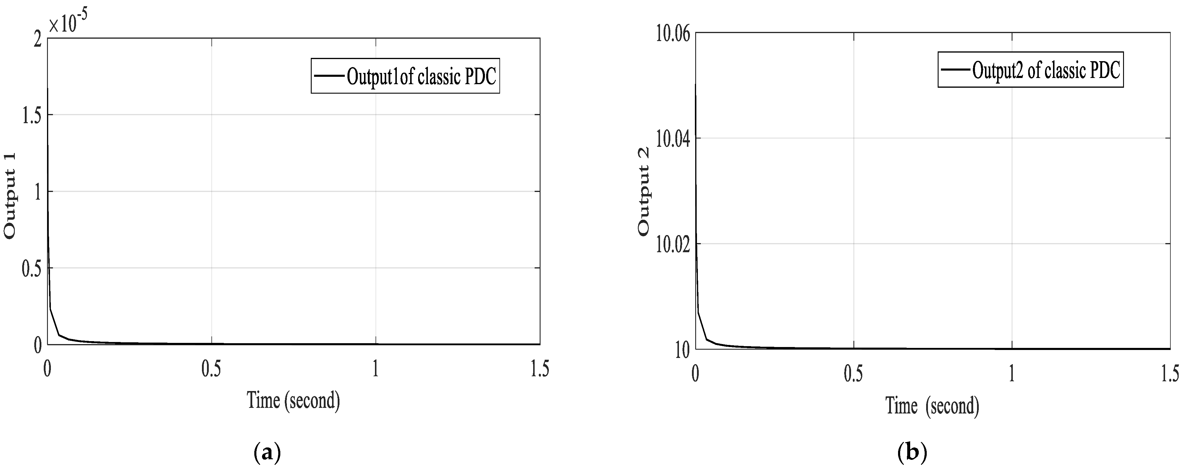
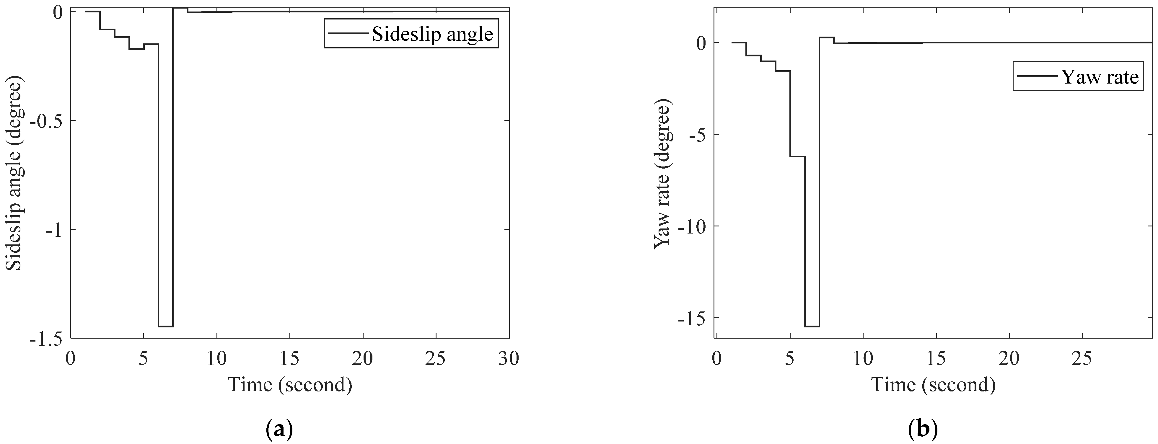
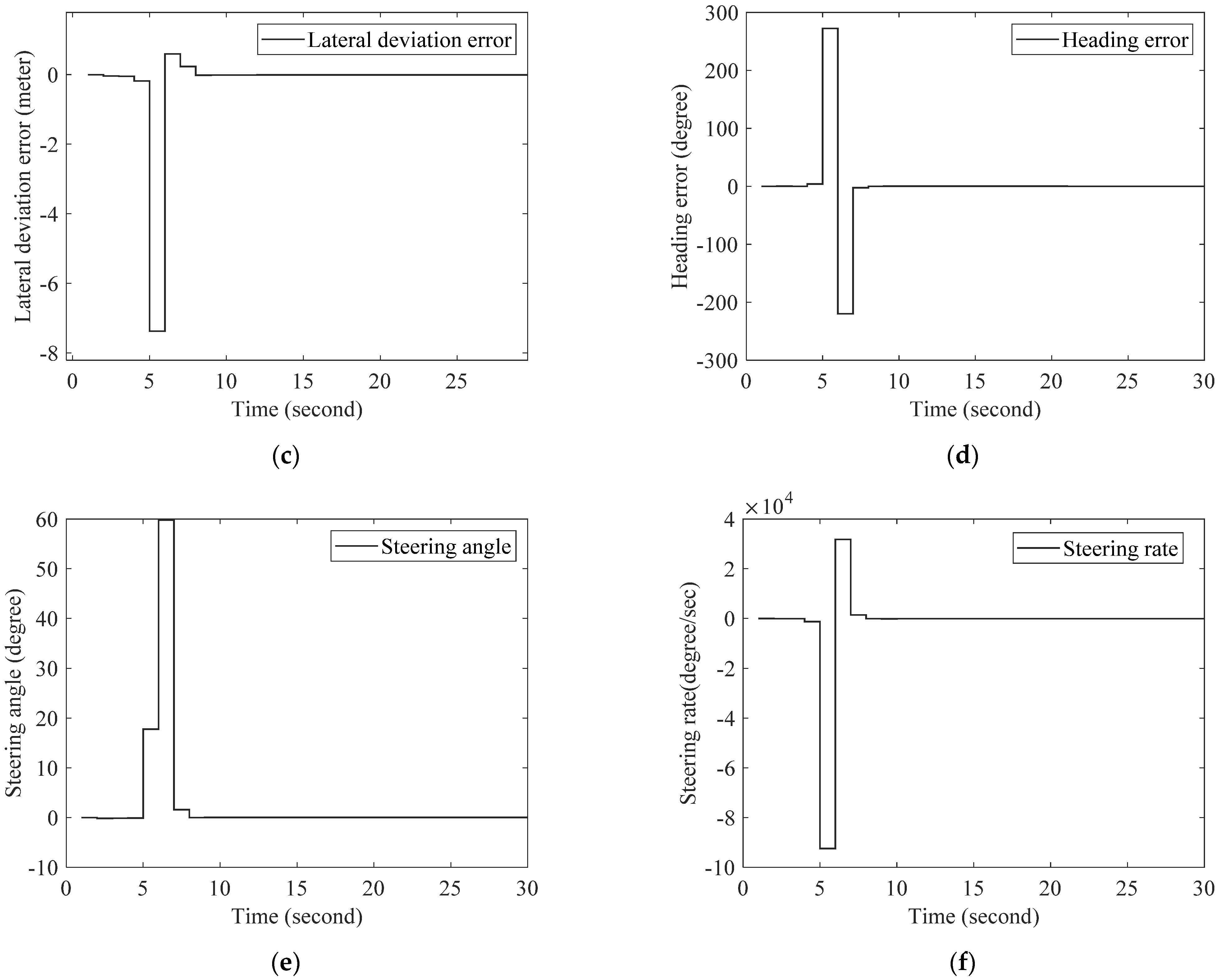
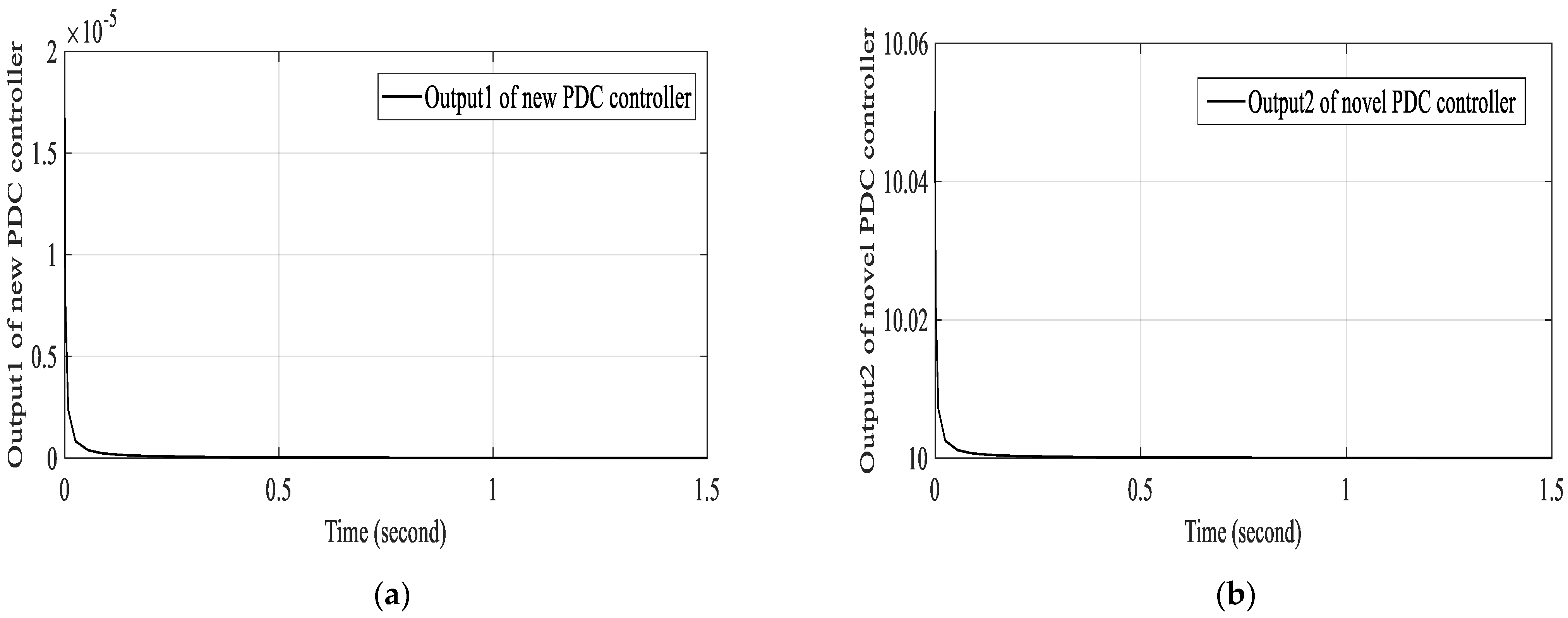
Firstly, we test the control input saturation, which means that we make the assumption that the vehicle system will not start from the origin. The state vector ${\mathrm{x}}_0=\left[0;0.01;0.02;0;0;0.3\right]$, which is not the system equilibrium points, for example, the lane centreline. It can be clearly observed that our two T-S systems converge all the state variables to zero, but the system control based on the new PDC law formulation converges faster and shows more robustness than the first T-S controller shows. The system dynamic is subjected to a lateral wind force of 500 Newton. Figure 2 of the classic PDC controller shows a remarkable robust stabilization. The six states given by the classic PDC controller are illustrated in Figure 3. Figure 4 presents the stabilization based on the new PDC controller. Figure 5 of the new PDC control design, shows that the six states converge to the equilibrium point zero, which proves that the autonomous vehicle is in the centreline of the lane. In others, our model is tested in terms of disturbance mitigation. Our model showed robustness and effectiveness against disturbances.

As shown in the following figures, the new PDC controller stabilizes the state vector variable faster than the classic PDC controller does.

Table 2. Comparison between states time convergence.

States	Classic PDC (second)	Improved PDC (second)
Sideslip	10	7
Yaw rate	12	11
Lateral deviation	8	8
Heading error	8	8
Steering angle	8	8
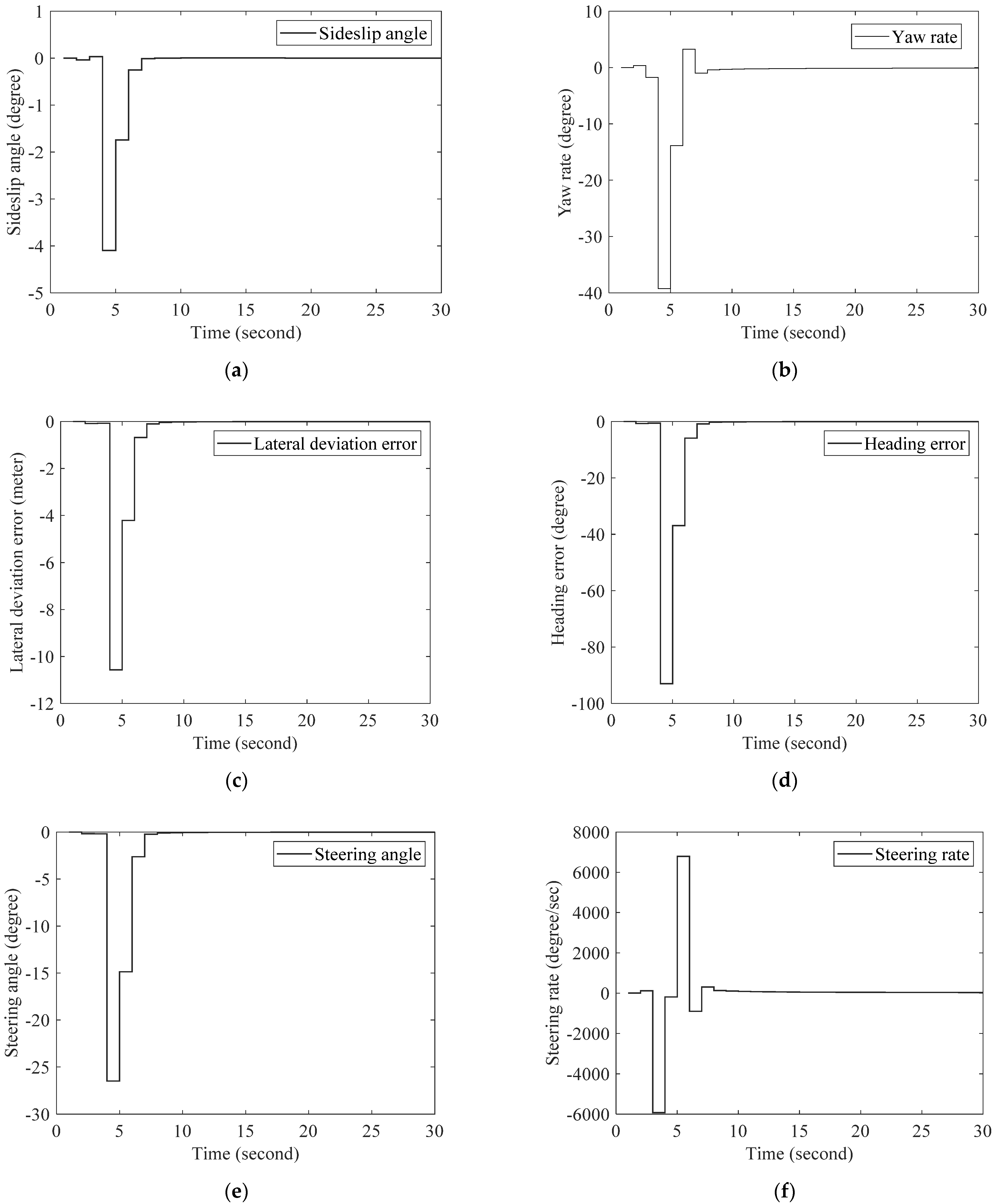
Steering rate	8	10

below shows that the sideslip angle converges to zero. It takes 10 s when using the classic PDC controller and 7 s when using the new PDC controller design. The yaw rate converges in 12 s using the classic PDC controller while it takes 11 s using the new PDC controller. The lateral deviation and the heading error share the same time for both cases as well as the steering angle; however, it can be observed that the behavior of the lateral deviation error of the new PDC controller is better than the classic one, because we do not have an overshoot in this case. As seen in Figure 3d, the heading error was 290 degree using the classic PDC controller, while in Figure 5d; the heading error is only 95 degree using the new PDC controller. This implies a reduction of 67.24 percent. On the other hand, the steering rate takes 8 s for the classic PDC, while it takes 10 s for the new PDC design. Nevertheless, the improvement is in the term of degree per second, which is better than the case of the new PDC controller.

These results confirm the robustness and the effectiveness in terms of stabilization and improvement of lateral control as shown in the previous figures. We notice also that all trajectories of the vehicle T-S fuzzy system converge to zero.

6. Conclusions

We proposed in this paper an improved Parallel Distributed Compensation law for lateral control purpose, suggesting new steering control architecture of autonomous vehicles. The vehicle system has been defined by discrete-time T-S model. This method relies on the use of a quadratic Lyapunov function, which is easy to implement, and LMIs techniques for the optimization goal, in particular to get the matrices and gains values that ensures the global asymptotic stability of the system and the multiobserver. We also computed the true values of the state vector using multiple Luenberger observers. Moreover, in this paper, we compared the lateral control results given by the new formulation of the PDC law with the improved classic one [21]. As shown, the two lateral controllers converge the autonomous vehicles states to the equilibrium point and ensure the lane keeping under various constraints. In this paper, the improved PDC control law ensures relaxed results, and faster convergence comparing to the classic one. This method is simple and effective than the nonquadratic methods presented previously in some references [5,6,7] in this paper. This method can be a real interest in other related applications e.g., drone control, underwater autonomous vehicles and autonomous ship control. The effectiveness of the proposed method is clearly illustrated via different figures.

References

- Herrmann, A.; Brenner, W.; Stadler, R. Autonomous Driving: How the Driverless Revolution Will Change the World; Emerald Group Publishing: Bingley, UK, 2018. [Google Scholar]
- Nguyen, A.T.; Coutinho, P.; Guerra, T.M.; Palhares, R.; Pan, J. Constrained Output-Feedback Control for Discrete-Time Fuzzy Systems with Local Nonlinear Models Subject to State and Input Constraints. IEEE Trans. Cybern. 2020, 51, 4673–4683. [Google Scholar] [CrossRef] [PubMed]
- Ling, S.; Wang, H.; Liu, P.X. Adaptive Fuzzy Tracking Control of Flexible-Joint Robots Based on Command Filtering. IEEE Trans. Ind. Electron. 2020, 67, 4046–4055. [Google Scholar] [CrossRef]
- Li, W.; Xie, Z.; Wong, P.K.; Mei, X.; Zhao, J. Adaptive-event-trigger-based fuzzy nonlinear lateral dynamic control for autonomous electric vehicles under insecure communication networks. IEEE Trans. Ind. Electron. 2020, 68, 2447–2459. [Google Scholar] [CrossRef]
- Nguyen, A.T.; Sentouh, C.; Popieul, J.C. Takagi-sugeno model-based steering control for autonomous vehicles with actuator saturation. IFAC-PapersOnLine 2016, 49, 206–211. [Google Scholar] [CrossRef]
- Nguyen, A.T.; Sentouh, C.; Popieul, J.C. Fuzzy steering control for autonomous vehicles under actuator saturation: Design and experiments. J. Frankl. Inst. 2018, 355, 9374–9395. [Google Scholar] [CrossRef]
- Sentouh, C.; Nguyen, A.-T.; Benloucif, M.A.; Popieul, J.-C. Driver-Automation Cooperation Oriented Approach for Shared Control of Lane Keeping Assist Systems. IEEE Trans. Control Syst. Technol. 2018, 27, 1962–1978. [Google Scholar] [CrossRef]
- Naranjo, J.E.; González, C.; García, R.; De Pedro, T.; Haber, R.E. Power-steering control architecture for automatic driving. IEEE Trans. Intell. Transp. Syst. 2005, 6, 406–415. [Google Scholar] [CrossRef] [Green Version]
- Du, H.; Zhang, N.; Dong, G. Stabilizing vehicle lateral dynamics with considerations of parameter uncertainties and control saturation through robust yaw control. IEEE Trans. Veh. Technol. 2010, 59, 2593–2597. [Google Scholar]
- Sun, W.; Wang, X.; Zhang, C. A model-free control strategy for vehicle lateral stability with adaptive dynamic programming. IEEE Trans. Ind. Electron. 2019, 67, 10693–10701. [Google Scholar] [CrossRef]
- Li, D.; Zhao, D.; Zhang, Q.; Chen, Y. Reinforcement learning and deep learning based lateral control for autonomous driving [application notes]. IEEE Comput. Intell. Mag. 2019, 14, 83–98. [Google Scholar] [CrossRef]
- Jiang, J.; Astolfi, A. Lateral control of an autonomous vehicle. IEEE Trans. Intell. Veh. 2018, 3, 228–237. [Google Scholar] [CrossRef] [Green Version]
- Liu, M.; Chour, K.; Rathinam, S.; Darbha, S. Lateral control of an autonomous and connected vehicle with limited preview information. IEEE Trans. Intell. Veh. 2020, 6, 406–418. [Google Scholar] [CrossRef]
- Zhang, H.; Wang, J. Vehicle Lateral Dynamics Control through AFS/DYC and Robust Gain-Scheduling Approach. IEEE Trans. Veh. Technol. 2015, 65, 489–494. [Google Scholar] [CrossRef]
- Hwang, Y.; Kang, C.M.; Kim, W. Robust Nonlinear Control Using Barrier Lyapunov Function Under Lateral Offset Error Constraint for Lateral Control of Autonomous Vehicles. IEEE Trans. Intell. Transp. Syst. 2020, 1–7. [Google Scholar] [CrossRef]
- Huang, Y.; Yong, S.Z.; Chen, Y. Stability Control of Autonomous Ground Vehicles Using Control-Dependent Barrier Functions. IEEE Trans. Intell. Veh. 2021, 6, 699–710. [Google Scholar] [CrossRef]
- Tong, S.; Min, X.; Li, Y. Observer-Based Adaptive Fuzzy Tracking Control for Strict-Feedback Nonlinear Systems With Unknown Control Gain Functions. IEEE Trans. Cybern. 2020, 50, 3903–3913. [Google Scholar] [CrossRef] [PubMed]
- Jiang, B.; Karimi, H.R.; Kao, Y.; Gao, C. Adaptive control of nonlinear semi-Markovian jump T–S fuzzy systems with immeasurable premise variables via sliding mode observer. IEEE Trans. Cybern. 2018, 50, 810–820. [Google Scholar] [CrossRef] [Green Version]
- Hua, H.; Cao, J.; Yang, G.; Ren, G. Voltage control for uncertain stochastic nonlinear system with application to energy Internet: Non-fragile robust H ∞ approach. J. Math. Anal. Appl. 2018, 463, 93–110. [Google Scholar] [CrossRef]
- Hua, H.; Qin, Y.; He, Z.; Li, L.; Cao, J. Energy sharing and frequency regulation in energy network via mixed H2/H∞ control with Markovian jump. CSEE J. Power Energy Syst. 2021, 7, 1302–1311. [Google Scholar]
- Jemmali, M.A.; Otis, M.J.-D.; Ellouze, M. Robust stabilization for discrete-time Takagi-Sugeno fuzzy system based on N4SID models. Eng. Comput. 2019, 36, 1400–1427. [Google Scholar] [CrossRef]
- Rajamani, R. Vehicle Dynamics and Control; Springer: Boston, MA, USA, 2012. [Google Scholar]
- Jiang, J.; Astolfi, A. Shared-Control for the Lateral Motion of Vehicles. In Proceedings of the European Control Conference (ECC), Limassol, Cyprus, 12–15 June 2018; pp. 225–230. [Google Scholar]
- Boyd, S.; El Ghaoui, L.; Feron, E.; Balakrishnan, V. “Linear matrix inequalities in system and control theory” SIAM studies in applied and numerical mathematics. In Society for Industrial and Applied Mathematics; SIAM: Philadelphia, PA, USA, 1994; Volume 15. [Google Scholar]
- Tanaka, K.; Nishimura, M.; Wang, H.O. Multi-objective fuzzy control of high rise/high speed elevators using LMIs. In Proceedings of the 1998 American Control Conference, ACC, Philadelphia, PA, USA, 26 June 1998; Volume 6, pp. 3450–3454. [Google Scholar]
- Nguyen, H.T.; Sugeno, M. (Eds.) Fuzzy Systems, Modelling and Control; Kluwer Academic Publisher: New York, NY, USA, 1988. [Google Scholar]
- Kim, E.; Lee, H. New approaches to relaxed quadratic stability condition of fuzzy control systems. IEEE Trans. Fuzzy Syst. 2000, 8, 523–534. [Google Scholar]
- Tanaka, K.; Ikeda, T.; Wang, H. Fuzzy regulators and fuzzy observers: Relaxed stability conditions and LMI-based designs. IEEE Trans. Fuzzy Syst. 1998, 6, 250–265. [Google Scholar] [CrossRef] [Green Version]
- Tanaka, K.; Wang, H.O. Fuzzy Control Systems Design and Analysis: A Linear Matrix Inequality Approach; Wiley, Wiley-Interscience: New York, NY, USA, 2004. [Google Scholar]
Figure 1.
Lateral vehicle dynamics modeling.
Figure 2.
PDC lateral controller stabilization of the autonomous vehicle under wind force: (a) Output1 of the autonomous vehicle; (b) Output2 of the autonomous vehicle.
Figure 3.
The stabilization of the autonomous vehicle six states using the classic PDC control law: (a) Sideslip using the classic PDC law; (b) Yaw rate using the classic PDC law; (c) Lateral deviation error using the classic PDC law; (d) Description of what is contained Heading error using the classic PDC law; (e) Steering angle using the classic PDC law; (f) Steering rate using the classic PDC law.
Figure 4.
The improved PDC lateral controller stabilization of the autonomous vehicle under wind force: (a) Output1 of the autonomous vehicle; (b) Output2 of the autonomous vehicle.
Figure 5.
The stabilization of the autonomous vehicle six states using the improved PDC control law: (a) Sideslip using the improved PDC law; (b) Yaw rate using the improved PDC law; (c) Lateral deviation error using the improved PDC law; (d) Description of what is contained Heading error using the improved PDC law; (e) Steering angle using the improved PDC law; (f) Steering rate using the improved PDC law.