Distribution Contract Analysis on e-Platform by Considering Channel Role and Good Complementarity

Abstract

Although suppliers can sell their goods on e-retailers’ e-platforms through either a wholesale or agency contract, suppliers that produce complementary goods and have different channel roles have been confused as to how to choose an optimal distribution contract. This paper aims to study this problem by considering the combined impacts of suppliers’ channel roles, e-retailer’s referral fees, goods’ differences in the level of complementarity and goods’ differences in potential demand. Our results show that, regardless of one supplier’s distribution contract choice, the other supplier always prefers agency contract, which is independent of two suppliers’ channel roles, the e-retailer’s referral fees, two goods’ differences in the level of complementarity and two goods’ differences in the potential demand. Moreover, when two suppliers use different distribution contracts to sell goods with different levels of complementarity on the same e-retailer’s e-platform, low-complementarity goods have a larger optimal retail price only if the two goods’ differences in the level of complementarity are sufficiently high, and the supplier can obtain more profits by producing low-complementarity goods regardless of the supplier’s distribution contract and channel role.

1. Introduction

E-platforms have been developing rapidly in the past few years, and an increasing number of consumers have begun purchasing goods from e-platforms. For example, consumers in China spent 10.63 trillion yuan on online shopping in 2019, which is an increase of 17.98% from 2018 (Site 1. The websites used in this paper are listed in Appendix A). Consumers in the U.S. spent $601.75 billion on online shopping in 2019 (Site 2), and eMarketer predicted that U.S. consumers’ expenses on online shopping will rise to $668.50 billion in 2020 (Site 3). In practice, many suppliers produce complementary goods and sell them on one e-retailer’s e-platform. The e-retailer provides two contracts for suppliers to use its e-platform. One is an agency contract (A contract), where suppliers set their goods’ retail prices and sell the goods directly to consumers through the e-retailer’s e-platform but need to share a proportion of their sales revenue (referral fees) to the e-retailer [1,2,3], and the e-retailer charges different referral fees to suppliers that produce different categories of goods. The other is a wholesale contract (W contract), where suppliers wholesale their goods to the e-retailer that then announces the retail prices and sells the goods to consumers on its e-platform [4,5,6]. An A contract makes the e-retailer charge referral fees to suppliers but enables it to lose the right to decide retail prices [7], and a W contract provides the e-retailer with the right to decide retail prices but makes it undertake the sales work [3].

There are many suppliers that produce complementary goods, selling the goods on one common e-retailer’s e-platform. For example, Apple uses a W contract to sell mobile phones on JD’s e-platform, and Vivo also uses a W contract to sell headsets on JD’s e-platform; Caluola uses an A contract to sell watches on JD’s e-platform, and FB also uses an A contract to sell batteries on JD’s e-platform. Chaoyang uses an A contract to sell tires on JD’s e-platform, whereas Jeep uses a W contract to sell bicycles on JD’s e-platform. However, are the distribution contracts used by these suppliers the most beneficial to them? An A contract gives suppliers the right to decide retail prices and provides suppliers with direct access to consumers but makes them pay referral fees to the e-retailer [1], and a W contract deprives suppliers of the right to decide retail prices but makes them relegate sales work to the e-retailer [3]. Thus, for suppliers that produce complementary goods, it is common to sell the goods on the same e-retailer’s e-platform, and how to choose the optimal distribution contract confuses them. However, to date, no researchers have explored the distribution contract choice of these suppliers.

For suppliers that sell complementary goods on one common e-retailer’s e-platform, one supplier’s distribution contract choice will lead to the other suppliers’ different strategic reactions. This is mainly because suppliers’ different distribution contracts will bring about different decision-makers of retail price, which eventually affects the e-retailer’s and suppliers’ profits and consumers’ demands. Therefore, when one supplier chooses the distribution contract, it should consider other suppliers’ reactions. Moreover, suppliers have “power”, defined by [8] as “the ability of one channel member to control the decision variables in the marketing strategy of another member in a given channel”. Different suppliers are different in their power, which leads to them having different channel roles; specifically, one that has more power can be the channel leader, whereas the other can be the channel follower [9,10]. For example, on JD’s e-platform, Renault, one of the Fortune Global 500, sells watches, and Camelion sells batteries. Undoubtedly, Renault has more power than Camelion, and thus, Renault is the channel leader. Some studies (e.g., [11,12,13]) use a Stackelberg game to characterize different suppliers’ channel roles; specifically, the channel leader is assumed to be the Stackelberg leader, and the channel follower is assumed to be the Stackelberg follower. How do suppliers’ different channel roles affect their distribution contract choices, pricing decisions and profits? This has confused suppliers that produce complementary goods and have different channel roles. However, there are no studies on this issue so far.

The objectives of this paper are to analyze the effects of suppliers’ different distribution contracts on the channel members’ pricing decisions and profits, and study the impacts of suppliers’ different channel roles on suppliers’ distribution contract choices, pricing decisions and profits. To achieve the objectives of this article, we focus on a supply chain (SC) with two suppliers (supplier 1 and supplier 2) and one e-retailer that has an e-platform, and the two suppliers have different channel roles. Without loss of generality, we assume supplier 1 is the channel leader, and supplier 2 is the channel follower. Each supplier produces a good, and the two goods are functionally complementary. The e-retailer offers each supplier two contracts to sell goods on the e-platform: an A contract and a W contract. We establish four game models to characterize two suppliers’ distribution contracts and their channel roles as follows: (I) two suppliers both use a W contract; (II) supplier 1 uses a W contract, and supplier 2 uses an A contract; (III) supplier 1 uses an A contract, and supplier 2 uses a W contract; and (IV) two suppliers both use an A contract.

The rest of the paper is organized as follows. Section 2 reviews the relevant literature. Section 3 presents the models and the analytic results. Comparisons of the models’ analytic results and managerial implications are presented in Section 4. Section 5 summarizes the results and gives future research directions.

2. Literature Review

Literature related to our study can be categorized into two streams: e-platforms and complementary goods, which are discussed in the following section.

2.1. E-Platforms

An emerging body of literature focuses on e-platforms from various perspectives. Specifically, some studies (e.g., [1,2,6,7]) analyze the interactions between distribution contracts on e-platforms and traditional distribution contracts. Moreover, Wang et al. [14] explore distribution contract choice on the e-platform when the supplier sells goods through both its online direct channel and the e-retailer’s e-platform, and Yan et al. [3] examine the strategy regarding whether to introduce an A contract in addition to the existing W contract. Other studies (e.g., [5,15,16]) explore distribution contract choice on e-platforms without considering existing distribution contracts, and our study also examines it. Specifically, Tian et al. [5] and Zennyo [16] consider an SC including one e-retailer and two suppliers that produce substitutable goods. Tian et al. [5] show that when the two suppliers choose the same distribution contract, their optimal choices depend on the competition intensity instead of the referral fees. Zennyo [16] finds that the supplier that produces high-demand goods can choose a preferred one between A and W contracts, but the supplier that produces low-demand goods has no choice but to accept the A contract. Furthermore, Wei et al. [15] consider an SC with one supplier selling a single good through two e-retailers’ e-platforms, and demonstrate that regardless of the supplier’s choice on one e-platform, its optimal choice on the other e-platform is always A contract. The differences between these studies and our study are summarized in

Table 1. Articles on e-platforms.

Articles	Decision-Maker	HCR	Product Status	Problem
[1]	One S and two Es	Same	Single	E’s decision on using A or W contract in addition to traditional distribution channel
[2]	One S, one RE and one E	Same	Substitutable	SC members’ decisions on using A or W contract in the presence of traditional distribution channel
[6]	One S and one E	N/A	Single	Whether to introduce A contract in addition to W contract and traditional distribution channel
[7]	One S and one E	N/A	Single	Whether to introduce traditional distribution channel in addition to A or W contract
[14]	One S and one E	N/A	Single	A or W contract to complement the S’s online direct channel
[3]	One S and one E	N/A	Single	Whether to introduce A contract in addition to W contract
[5]	Two Ss and one E	Same	Substitutable	A or W contract
[15]	One S and Two Es	Different	Single	A or W contract
[16]	Two Ss and one E	Same	Substitutable	A or W contract
Our study	Two Ss and one E	Different	Complementary	A or W contract

Note: where S, E and RE represent the supplier, the e-retailer and the retailer, respectively, and HCR denotes the horizontal channel role.

.

Unlike the above research which focuses on e-platforms where a single good or substitutable goods are sold, our study is the first one to focus on e-platforms with complementary goods. Furthermore, nearly half of literature examines a one-to-one SC, and the other literature except [15] is performed in two-to-one or one-to-two SC structure, and only considers the scenario in which SC members in the same echelon (downstream or upstream) have same channel role. Wei et al. [15] explore distribution contract choice in an SC with one supplier and two e-retailers that have different channel roles, but our study investigates it in an SC with one e-retailer and two suppliers that have different channel roles. Our results show that when two suppliers sell complementary goods on one e-retailer’s e-platform, no matter what distribution contract one supplier chooses, the other supplier always prefers an A contract, which is independent of the two suppliers’ channel roles, the e-retailer’s referral fees, two goods’ differences in the level of complementarity and two goods’ differences in the potential demand.

2.2. Complementary Goods

Complementary goods have been extensively explored in numerous studies. Literature on this topic proceeds from various perspectives, such as information sharing (e.g., [13,17,18]), product promotion (e.g., [19,20]), joint selling (e.g., [21,22,23]), recycling channel decision (e.g., [24]), mechanism design (e.g., [25]) and pricing problems (e.g., [10,26,27]). Our study is situated in the research stream of pricing problems. In this stream of literature, Ren et al. [26] explore the impacts of trade credit on the pricing decisions of complementary goods, and find that the impacts of trade credit on SC members’ profits depend on the difference in the opportunity cost between the suppliers that extend trade credit and the retailer. Wang et al. [27] investigate complementary goods’ pricing decisions when the retailer provides services to consumers, and reveal that it is not profitable for the retailer to improve its service level infinitely. Wei et al. [10] study complementary goods’ pricing decisions by considering SC members’ market power structures, and illustrate that an increase in potential demand always increases the optimal retail prices regardless of SC members’ market power structures. Moreover, all of this research is conducted under the scenario where the manufacturer adopts the traditional distribution and online direct channels simultaneously or under the scenario where the manufacturer adopts only the traditional distribution channel.

Different from the above literature regarding complementary goods, our study considers an SC including two suppliers and one e-retailer that has an e-platform, and the two suppliers can use a W or A contract to sell complementary goods on the e-retailer’s e-platform, which results in different decision-makers of retail price, and this eventually affects the SC members’ pricing decisions and profits. Moreover, different suppliers have different channel roles, which leads to different price decisions, and this ultimately has an impact on the suppliers’ profits and distribution contract choices. However, in the context of complementary goods, no researchers consider distribution contracts on e-platforms, and there is also no research on how the interaction between suppliers’ different channel roles and their distribution contracts on e-platforms affects the SC members’ pricing decisions and profits. Our study attempts to fill this research gap. We find that when two suppliers use different distribution contracts to sell goods with different levels of complementarity on the same e-retailer’s e-platform, low-complementarity goods have a larger optimal retail price only if the two goods’ differences in the level of complementarity are sufficiently high and the supplier can obtain more profits by producing low-complementarity goods regardless of its distribution contract and channel role.

3. Models and Analytic Results

This paper focuses on an SC including two suppliers (supplier 1 and supplier 2) that are SC followers, and one e-retailer that is an SC leader. Supplier $i$ produces good $i$ at unit manufacturing cost $c_i,i=1,2$, and the two goods are functionally complementary. The e-retailer possesses an e-platform, and each supplier can use an A or W contract to sell complementary goods on the e-retailer’s e-platform. Based on the above SC structure, we intend to gain an understanding of the interaction between the two suppliers’ channel roles and their distribution contracts on the same e-retailer’s e-platform by addressing the following issues: (1) how do suppliers’ different distribution contracts affect the channel members’ pricing decisions and profits facing different channel roles? (2) Given suppliers’ distribution contracts, how do the suppliers’ channel roles affect the channel members’ pricing decisions and profits? (3) As the leader of a supply chain, how does the e-retailer guide suppliers to choose distribution contracts?

To answer the above questions, we first establish a WWS1 model to characterize Scenario I where two suppliers both use a W contract to sell complementary goods on the same e-retailer’s e-platform. We then formulate a WAS1 model to characterize Scenario II where a powerful supplier (supplier 1) uses a W contract and a small supplier (supplier 2) uses an A contract, and the small supplier needs to pay a proportion, denoted by $\varphi$, of its sales revenue to the e-retailer which is widely used in the research on e-platforms (e.g., [4,16,28]). Next, we formulate an AWS1 model to characterize scenario III, where a powerful supplier uses an A contract and a small supplier uses a W contract, and the powerful supplier needs to pay a proportion, denoted by $\varphi$, of its sales revenue to the e-retailer. Finally, we use an AAS1 model to characterize Scenario IV where two suppliers both use an A contract, and each supplier should pay referral fees to the e-retailer. For clarity, we summarize the four game models in

Table 2. The four game models.

Supplier 2
Supplier 1		W contract	A contract
	W contract	WWS1	WAS1
	A contract	AWS1	AAS1

.

Moreover, in every model, we assume supplier 1 is the channel leader, and supplier 2 is the channel follower. In alignment with [11,12,13], we use a Stackelberg game to characterize two suppliers’ channel roles; specifically, the channel leader is assumed to be Stackelberg leader, and the channel follower is assumed to be Stackelberg follower. We also assume the e-retailer and both suppliers are risk-neutral and information-complete [2,15,28], and each SC member makes its decisions by maximizing its own profit [5,14,29]. For the demand functions, we assume the two goods’ demand functions are linearly price-dependent, which is commonly used in the literature (e.g., [7,16,29,30,31]). The demands for goods 1 and 2 are $D_1=a_1-p_1-{\gamma }_1{p}_2$ and $D_2=a_2-p_2-{\gamma }_2{p}_1$, respectively, where $a_i$ denotes good $i$’s potential demand (i.e., market base of good $i$ if free of charge). The parameter ${\gamma }_i$ denotes the level of complementarity between two goods, and satisfies $0<{\gamma }_i<1$ which means that a good’s demand is more sensitive to changes in its own price than to changes in the price of its complementary good. A greater value of ${\gamma }_i$ represents a higher level of complementarity between two goods.

3.1. The WWS1 Model

In this model, the e-retailer (e.g., JD) purchases good 1 (e.g., watches) from supplier 1 (e.g., Longines) at unit wholesale price $w_1$, and then resells them to consumers at unit retail price $p_1$. Moreover, the e-retailer (e.g., JD) purchases good 2 (e.g., batteries) from supplier 2 (e.g., Camelion) at unit wholesale price $w_2$, and then resells them to consumers at unit retail price $p_2$. The profit functions of supplier $i$ (${\pi }_{si}(w_i)$) and the e-retailer (${\pi }_e(p_1,p_2)$) are

$${\pi }_{si}(w_i)=(w_i-c_i)(a_i-p_i-{\gamma }_i{p}_j),j=3-i,i=1,2,$$

(1)

$${\pi }_e(p_1,p_2)=(p_1-w_1)(a_1-p_1-{\gamma }_1{p}_2)+(p_2-w_2)(a_2-p_2-{\gamma }_2{p}_1).$$

(2)

The e-retailer, as the whole SC leader, first simultaneously announces retail prices $p_1$ and $p_2$; then, supplier 1, as the channel leader of two suppliers, determines wholesale price $w_1$, and finally, supplier 2 sets wholesale price $w_2$ to maximize its profit function. Similar to [1,26,32], the results of Proposition 1 are derived by backward induction. The proofs of Proposition 1 and other propositions are given in Appendix B.

Proposition 1. 

In the WWS1 model, supplier 1’s and supplier 2’s optimal wholesale prices$w_1^{WWS1*}$ and $w_2^{WWS1*}$, and the e-retailer’s optimal retail prices $p_1^{WWS1*}$ and $p_2^{WWS1*}$ are

$$\begin{gathered} w_1^{WWS1*}=\frac{a_1-p_1^{WWS1*}-{\gamma }_1{p}_2^{WWS1*}+(1-{\gamma }_1{\gamma }_2)c_1}{1-{\gamma }_1{\gamma }_2},w_2^{WWS1*}=a_2-p_2^{WWS1*}-{\gamma }_2{p}_1^{WWS1*}+c_2, \\ {p}_1^{WWS1*}=\frac{2(6-5{\gamma }_1{\gamma }_2)a_1-[{\gamma }_1(9-7{\gamma }_1{\gamma }_2)+{\gamma }_2(1-{\gamma }_1{\gamma }_2)]a_2+(1-{\gamma }_1{\gamma }_2)[(4-3{\gamma }_1{\gamma }_2-{\gamma }_1^2)c_1-(3{\gamma }_1-{\gamma }_2)c_2]}{(1-{\gamma }_1{\gamma }_2)(16-10{\gamma }_1{\gamma }_2-{\gamma }_1^2-{\gamma }_2^2)} \end{gathered}$$

and

$$\begin{gathered} p_2^{WWS1*}=\frac{2(6-6{\gamma }_1{\gamma }_2+{\gamma }_1^2{\gamma }_2^2)a_2-[{\gamma }_1(1-{\gamma }_1{\gamma }_2)+{\gamma }_2(9-7{\gamma }_1{\gamma }_2)]a_1-(1-{\gamma }_1{\gamma }_2)(3{\gamma }_2-{\gamma }_1-2{\gamma }_1{\gamma }_2^2)c_1}{(1-{\gamma }_1{\gamma }_2)(16-10{\gamma }_1{\gamma }_2-{\gamma }_1^2-{\gamma }_2^2)}+ \\ \frac{(4-{\gamma }_1{\gamma }_2-{\gamma }_2^2)c_2}{16-10{\gamma }_1{\gamma }_2-{\gamma }_1^2-{\gamma }_2^2}. \end{gathered}$$

From Proposition 1, when two suppliers both use a W contract to sell complementary goods on the same e-retailer’s e-platform, good $i$’s optimal retail price is positively correlated with its own potential demand and manufacturing cost, but is negatively correlated with the complementary good’s potential demand regardless of the two suppliers’ channel roles. Moreover, good $i$’s optimal wholesale price is not only negatively related to its own optimal retail price but also negatively related to the complementary good’s optimal retail price.

3.2. The WAS1 Model

In this model, the e-retailer (e.g., JD) not only wholesales goods (e.g., watches) from supplier 1 (e.g., Armani) at unit wholesale price $w_1$ and then resells them to consumers at unit retail price $p_1$, but also lets supplier 2 (e.g., Delipow) directly sell goods (e.g., batteries) to consumers at unit retail price $p_2$ on the e-platform by charging referral fees to supplier 2. The profit functions of supplier 1 (${\pi }_{s1}(w_1)$), supplier 2 (${\pi }_{s2}(p_2)$) and the e-retailer (${\pi }_e(p_1)$) are

$${\pi }_{s1}(w_1)=(w_1-c_1)(a_1-p_1-{\gamma }_1{p}_2),$$

(3)

$${\pi }_{s2}(p_2)=[(1-\varphi )p_2-c_2](a_2-p_2-{\gamma }_2{p}_1),$$

(4)

$${\pi }_e(p_1)=(p_1-w_1)(a_1-p_1-{\gamma }_1{p}_2)+\varphi p_2(a_2-p_2-{\gamma }_2{p}_1).$$

(5)

The timing of this subgame is as follows. The e-retailer first decides its profit-maximizing retail price $p_1$, then supplier 1 announces wholesale price $w_1$, and finally, supplier 2 sets retail price $p_2$. The results of Proposition 2 can be obtained by backward induction.

Proposition 2. 

In the WAS1 model, supplier 1’s optimal wholesale price$w_1^{WAS1*}$, supplier 2’s optimal retail price$p_2^{WAS1*}$and the e-retailer’s optimal retail price$p_1^{WAS1*}$are given as follows:

$$w_1^{WAS1*}=\frac{(1-\varphi )(2a_1-{\gamma }_1{a}_2)-{\gamma }_1{c}_2}{(1-\varphi )(2-{\gamma }_1{\gamma }_2)}+c_1-p_1^{WAS1*},p_2^{WAS1*}=\frac{(1-\varphi )(a_2-{\gamma }_2{p}_1^{WAS1*})+c_2}{2(1-\varphi )}$$

and

$$p_1^{WAS1*}=\frac{(1-\varphi )[6a_1-(3{\gamma }_1+\varphi {\gamma }_2)a_2+(2-{\gamma }_1{\gamma }_2)c_1]-3{\gamma }_1{c}_2}{(1-\varphi )(8-4{\gamma }_1{\gamma }_2-\varphi {\gamma }_2^2)}.$$

Proposition 2 indicates that (1) when supplier 1 uses a W contract and supplier 2 uses an A contract, the good’s optimal retail price under the W contract is positively related to its own potential demand and manufacturing cost, but is negatively related to the complementary good’s potential demand and manufacturing cost; (2) there is a negative relationship between e-retailer’s and supplier 2’s optimal retail prices, and this result is consistent with the assumption that the two goods are complementary; (3) the e-retailer’s optimal retail price is negatively correlated with supplier 1’s optimal wholesale price. Thus, when two suppliers use different distribution contracts, supplier 1 that uses a W contract hopes the e-retailer will sell the good at a low retail price.

3.3. The AWS1 Model

In this model, the e-retailer (e.g., JD) not only lets supplier 1 (e.g., Bonest Gatti) directly sell goods (e.g., watches) to consumers at unit retail price $p_1$ on the e-platform by charging referral fees to supplier 1, but also purchases goods (e.g., batteries) from supplier 2 (e.g., Sonlu) at unit wholesale price $w_2$ and then resells them to consumers at unit retail price $p_2$. The profit functions of supplier 1 (${\pi }_{s1}(p_1)$), supplier 2 (${\pi }_{s2}(w_2)$) and the e-retailer (${\pi }_e(p_2)$) are

$${\pi }_{s1}(p_1)=[(1-\varphi )p_1-c_1](a_1-p_1-{\gamma }_1{p}_2),$$

(6)

$${\pi }_{s2}(w_2)=(w_2-c_2)(a_2-p_2-{\gamma }_2{p}_1),$$

(7)

$${\pi }_e(p_2)=\varphi p_1(a_1-p_1-{\gamma }_1{p}_2)+(p_2-w_2)(a_2-p_2-{\gamma }_2{p}_1).$$

(8)

The e-retailer, as the SC leader, first sets retail price $p_2$, then supplier 1 announces retail price $p_1$, and finally, supplier 2 decides wholesale price $w_2$ to maximize its profit function. The results of Proposition 3 can be derived by backward induction.

Proposition 3. 

In the AWS1 model, supplier 1’s optimal retail price$p_1^{AWS1*}$, supplier 2’s optimal wholesale price$w_2^{AWS1*}$and the e-retailer’s optimal retail price$p_2^{AWS1*}$are given as follows:

$$p_1^{AWS1*}=\frac{(1-\varphi )(a_1-{\gamma }_1{p}_2^{AWS1*})+(1-{\gamma }_1{\gamma }_2)c_1}{(1-\varphi )(2-{\gamma }_1{\gamma }_2)},w_2^{AWS1*}=a_2-p_2^{AWS1*}-{\gamma }_2{p}_1^{AWS1*}+c_2$$

and

$$\begin{array}{l}{p}_2^{AWS1*}=\frac{(2-{\gamma }_1{\gamma }_2)(6-5{\gamma }_1{\gamma }_2)a_2-[{\gamma }_2(6-5{\gamma }_1{\gamma }_2)+2\varphi {\gamma }_1(1-{\gamma }_1{\gamma }_2)]a_1}{2(1-{\gamma }_1{\gamma }_2)(8-6{\gamma }_1{\gamma }_2-\varphi {\gamma }_1^2)}-\frac{{\gamma }_2(6-5{\gamma }_1{\gamma }_2-\varphi {\gamma }_1{}^2)c_1}{2(1-\varphi )(8-6{\gamma }_1{\gamma }_2-\varphi {\gamma }_1^2)}+\\ \frac{(2-{\gamma }_1{\gamma }_2)c_2}{(8-6{\gamma }_1{\gamma }_2-\varphi {\gamma }_1^2)}.\end{array}$$

Propositions 2 and 3 demonstrate that when two suppliers choose different distribution contracts, the optimal retail price of the good sold under the W contract has a positive relationship with its own potential demand and manufacturing cost but has a negative relationship with the complementary good’s potential demand and manufacturing cost. Proposition 3 also tells us that when supplier 1 uses an A contract and supplier 2 uses a W contract, the optimal retail price of supplier 1 is negatively related to that of the e-retailer, and supplier 2’s optimal wholesale price is negatively related to the e-retailer’s and supplier 1’s optimal retail prices.

3.4. The AAS1 Model

In this model, by charging referral fees, the e-retailer (e.g., JD) lets supplier 1 (e.g., Caluola) directly sell goods (e.g., watches) to consumers on the e-platform at unit retail price $p_1$, and lets supplier 2 (e.g., FB) directly sell goods (e.g., batteries) to consumers on the e-platform at unit retail price $p_2$. The profit functions of supplier $i$ (${\pi }_{si}(p_i)$) and the e-retailer (${\pi }_e$) are

$${\pi }_{si}(p_i)=[(1-\varphi )p_i-c_i](a_i-p_i-{\gamma }_i{p}_j),j=3-i,i=1,2,$$

(9)

$${\pi }_e=\varphi [p_1(a_1-p_1-{\gamma }_1{p}_2)+p_2(a_2-p_2-{\gamma }_2{p}_1)].$$

(10)

Supplier 1, as the Stackelberg leader of the two suppliers, first determines its profit-maximizing retail price $p_1$, and then supplier 2 sets retail price $p_2$. The results of Proposition 4 can be derived by backward induction.

Proposition 4. 

In the AAS1 model, supplier 1’s and supplier 2’s optimal retail prices$p_1^{AAS1*}$and$p_2^{AAS1*}$are given as follows:

$$p_1^{AAS1*}=\frac{(1-\varphi )(2a_1-{\gamma }_1{a}_2)+(2-{\gamma }_1{\gamma }_2)c_1-{\gamma }_1{c}_2}{2(1-\varphi )(2-{\gamma }_1{\gamma }_2)}$$

and

$$p_2^{AAS1*}=\frac{(1-\varphi )[(4-{\gamma }_1{\gamma }_2)a_2-2{\gamma }_2{a}_1]+(4-{\gamma }_1{\gamma }_2)c_2-{\gamma }_2(2-{\gamma }_1{\gamma }_2)c_1}{4(1-\varphi )(2-{\gamma }_1{\gamma }_2)}.$$

From Proposition 4, regardless of the two suppliers’ channel roles, when the two suppliers both use an A contract, good $i$’s potential demand and manufacturing cost positively affect its own optimal retail price but negatively affect the complementary good’s optimal retail price.

4. Comparison and Analysis of Results

The equilibrium solutions derived in the above four models are complex, and it is extremely difficult to obtain analytical results regarding all channel members’ decisions and profits thoroughly. Thus, using a numerical approach, we analyze the influences of several key factors (i.e., the e-retailer’s referral fees, two goods’ differences in the level of complementarity and two goods’ differences in the potential demand) on SC members’ decisions and profits to derive more managerial insights in this section.

To make the two suppliers and the e-retailer profitable in every model, the parameters $a_i$, ${\gamma }_i$, $c_i$ and $\varphi$ should satisfy some constraint conditions. For example, the parameters should make all SC members’ profit margins positive, make the two complementary goods’ manufacturing costs positive, make the two complementary goods’ demands positive, and so on. Specifically, the two complementary goods’ optimal retail/wholesale prices, manufacturing costs and maximum demands should satisfy $w_i^{WWS1*}>c_i>0$, $p_i^{WWS1*}>w_i^{WWS1*}$ and $D_i^{WWS1*}>0$ in the WWS1 model, satisfy $w_1^{WAS1*}>c_1>0$, $(1-\varphi )p_2^{WAS1*}>c_2>0$, $p_1^{WAS1*}>w_1^{WAS1*}$ and $D_i^{AWS1*}>0$ in the WAS1 model, satisfy $(1-\varphi )p_1^{AWS1*}>c_1>0$, $w_2^{AWS1*}>c_2>0$, $p_2^{AWS1*}>w_2^{AWS1*}$ and $D_i^{AWS1*}>0$ in the AWS1 model and satisfy $(1-\varphi )p_i^{AAS1*}>c_i>0$ and $D_i^{AAS1*}>0$ in the AAS1 model. However, due to the very complicated forms of the equilibrium solutions, it is impossible to obtain the analytic conditions for the parameters. Thus, in the following numerical studies, we apply the simulation method widely used in many studies (e.g., [3,29,33]) to choose appropriate parameter values to ensure that all SC members are profitable.

4.1. Impact of the e-Retailer’s Referral Fees

In this subsection, we explore how the SC members’ decisions and profits are affected by the e-retailer’s referral fees (characterized by $\varphi$). In practice, the value of $\varphi$ is the same for all goods within a certain category, and different values of $\varphi$ correspond to different categories of goods. To make sure the values of $\varphi$ are reasonable and convincing in our numerical studies, we have looked for the values of $\varphi$ used by many famous e-retailers for all categories of goods. Specifically, the values of $\varphi$ range from 6% to 20% for WalMart (Site 4), from 8% to 17% for Amazon (Site 5), from 1% to 10% for JD (Site 6), and so on. Thus, we take values of $\varphi$ from 1% to 20%. Moreover, the studies (e.g., [32,34]) show that two goods’ asymmetry will create problems when the models’ equilibrium solutions are compared. Thus, we simplify parameter structures (i.e., $a_1=a_2,$ $c_1=c_2$ and ${\gamma }_1={\gamma }_2$) to separate the impacts of two suppliers’ channel roles and distribution contracts from the impacts of each parameter’s difference. Moreover, we assume that the default values of these parameters are ${\gamma }_1={\gamma }_2=0.3,$ $a_1=a_2=150,$ $c_1=c_2=25$, and show the results in Figure 1, Figure 2 and Figure 3.

Discussion 1. 

Two suppliers may use the same or different distribution contracts to sell complementary goods with symmetric parameters on the common e-retailer’s e-platform. When two suppliers use the same distribution contract, we present the results in Figure 1 and Figure 2; for brevity, when two suppliers use different distribution contracts, we do not show the results in this article.

(1.1) 

If two suppliers use the same distribution contract to sell complementary goods with symmetric parameters, although the optimal retail/wholesale price of powerful supplier is remarkably larger than that of small supplier, there is no obvious difference between two suppliers’ profits. Thus, if two suppliers use the same distribution contract to sell complementary goods with symmetric parameters, although the leader role makes the supplier charge an obviously greater optimal retail/wholesale price, the leader role cannot make the supplier obtain obviously larger profits regardless of the referral fees; moreover, as the referral fees increase, the leader role’s advantage almost disappears when two suppliers both use an A contract.

(1.2) 

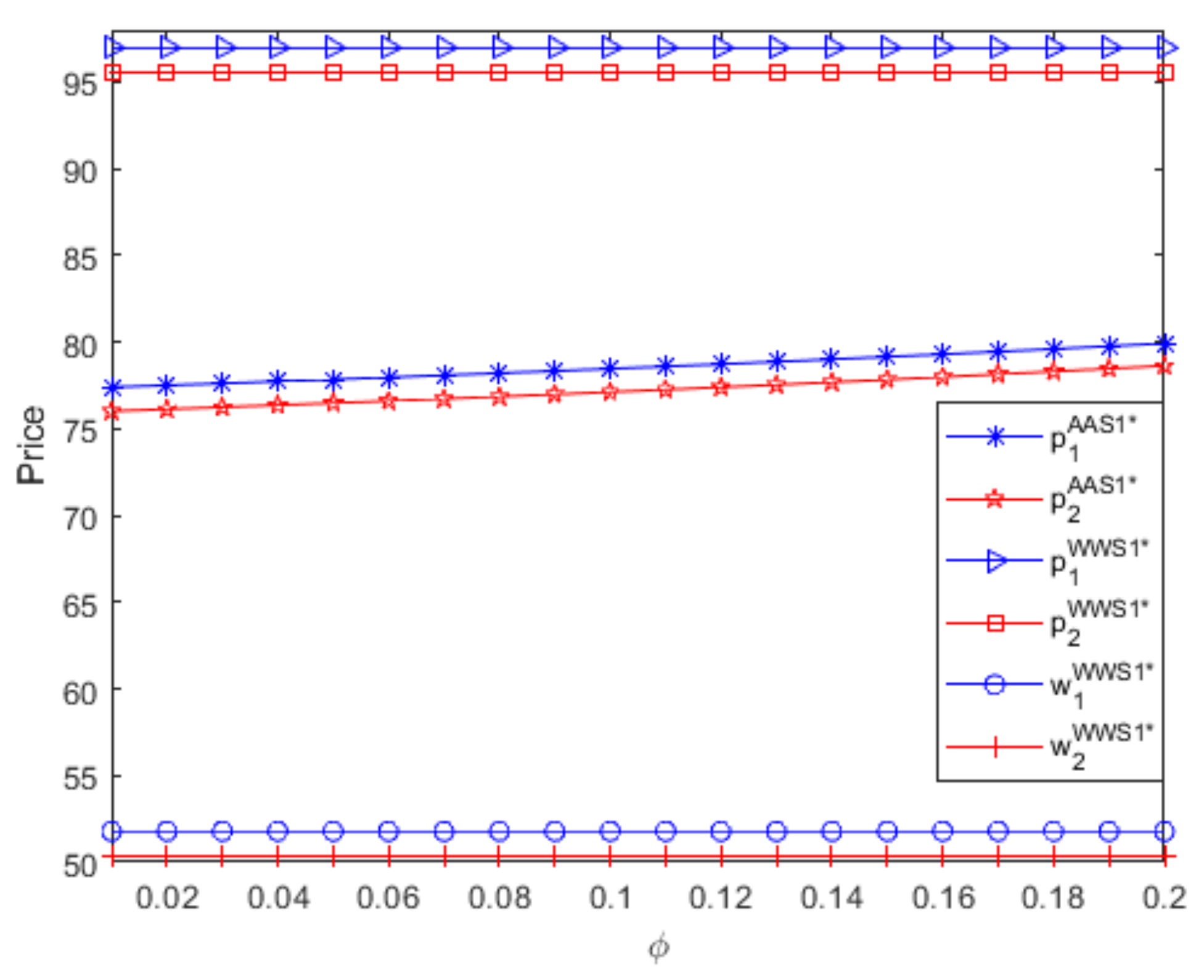
If two suppliers use the same distribution contract to sell complementary goods with symmetric parameters, although these goods have higher optimal retail prices when both suppliers use a W contract than when both suppliers use an A contract, two suppliers obtain more profits when they both use an A contract than when they both use a W contract, which is independent of the referral fees. Moreover, if two suppliers both use an A contract, as the referral fees increase, two goods’ optimal retail prices increase slowly, but two suppliers’ profits decrease quickly. If two suppliers use different distribution contracts to sell complementary goods with symmetric parameters, the optimal retail price charged in a W contract is larger than that charged in an A contract, and the supplier obtains more profits when it uses an A contract than when it uses a W contract, which is independent of its channel role and the referral fees. Thus, if two suppliers use the same or different distribution contracts to sell complementary goods with symmetric parameters, the optimal retail price charged by the e-retailer is greater than that charged by the supplier, and the A contract is more beneficial to the supplier than the W contract, which is independent of the referral fees.

Discussion 2. 

When two suppliers sell complementary goods with symmetric parameters, if one supplier uses an A or W contract, we analyze how the referral fees and the other supplier’s distribution contract affect the other supplier’s profit, and draw the following conclusions from Figure 2 and Figure 3.

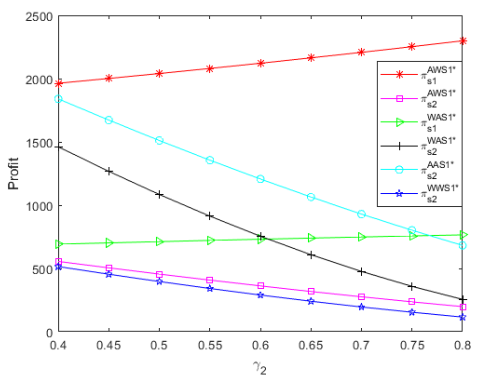
(2.1) 

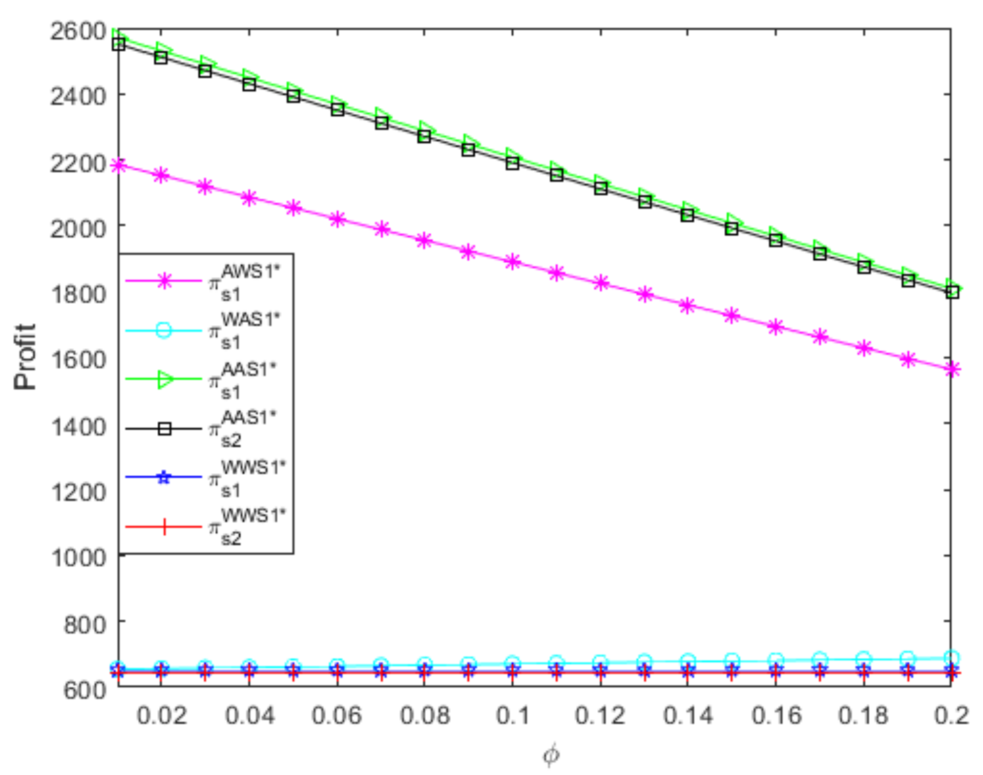
From Figure 2, if the small supplier uses an A contract, the profit of the powerful supplier using the A contract decreases as the referral fees increase, but the profit of the powerful supplier using the W contract increases as the referral fees increase; additionally, the A contract is more beneficial to the powerful supplier than the W contract, but the A contract’s advantage decreases as the referral fees increase. Moreover, if the small supplier uses the W contract, the profit of the powerful supplierusing the A contract decreases as the referral fees increase, while the profit of the powerful supplier using the W contract remains unchanged as the referral fees increase; additionally, the A contract is more beneficial to the powerful supplier than the W contract, but the A contract’s advantage decreases as the referral fees increase. Thus, regardless of the small supplier’s distribution contract, the impact of the referral fees on the powerful supplier’s profit depends on the powerful supplier’s distribution contract; additionally, the powerful supplier should choose the A contract, and the A contract’s advantage is larger when the referral fees are relatively low than when the referral fees are relatively high.

(2.2) 

From Figure 3, if the powerful supplier uses an A contract, the profit of the small supplier using the W contract increases as the referral fees increase, while the profit of the small supplier using the A contract decreases as the referral fees increase; additionally, the A contract is more beneficial to the small supplier than the W contract, but the A contract’s advantage decreases as the referral fees increase. Furthermore, if the powerful supplier uses the W contract, the profit of the small supplier using the A contract decreases as the referral fees increase, while the profit of the small supplier using the W contract remains unchanged as the referral fees increase; additionally, the A contract is more beneficial to the small supplier than the W contract, but the A contract’s advantage decreases as the referral fees increase. Thus, no matter what distribution contract the powerful supplier uses, the impact of the referral fees on the small supplier’s profit depends onthe small supplier’s distribution contract; additionally, the small supplier should choose the A contract, and the A contract’s advantage is greater when the referral fees are relatively low than when the referral fees are relatively high.

Discussion 3. 

When two suppliers sell complementary goods with symmetric parameters, we explore how the referral fees and the two supplier’s distribution contracts influence the e-retailer’s profit, and draw the following conclusions fromFigure 3.

(3.1) 

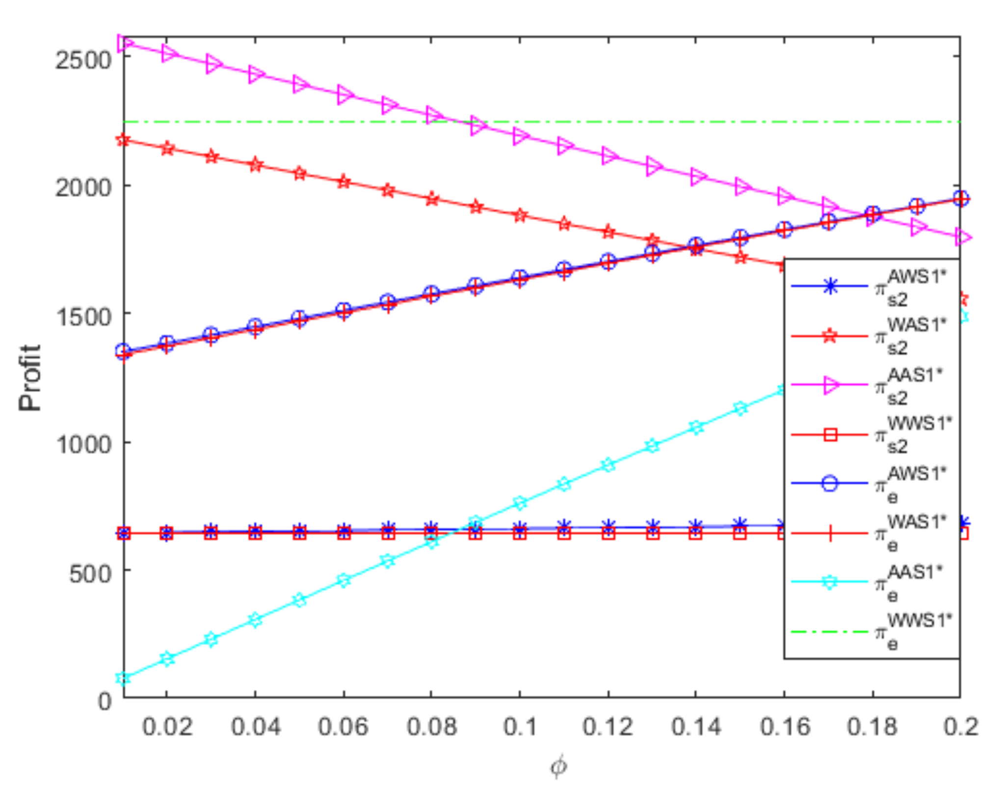
Regardless of the referral fees, the e-retailer achieves the highest profit when two suppliers both use a W contract to sell complementary goods with symmetric parameters. Moreover, if two suppliers use different distribution contracts to sell complementary goods with symmetric parameters, although the e-retailer obtains more profits when the powerful supplier uses an A contract and the small supplier uses a W contract than when the powerful supplier uses a W contract and the small supplier uses an A contract, the effect of the two suppliers’ different distribution contracts on the e-retailer’s profit is extremely small and almost disappears as the referral fees increase.

(3.2) 

If one supplier uses an A contract, although the referral fees have greater positive influences on the e-retailer’s profit when the other supplier also uses an A contract than when the other supplier uses a W contract, the other supplier’s W contract is always more beneficial to the e-retailer than the other supplier’s A contract, which leads to that W contract’s advantage decreases as the referral fees increase. Thus, if one supplier uses an A contract, the e-retailer should attempt to attract the other supplier to use a W contract, and the W contract’s advantage is greater when the referral fees are relatively low than when the referral fees are relatively high.

(3.3) 

If one supplier uses a W contract, although the e-retailer’s profit is always greater when the other supplier also uses the W contract than when the other supplier uses an A contract, the difference between the e-retailer’s profits under two distribution contracts decreases as the referral fees increase. Therefore, if one supplier uses a W contract, the e-retailer should attempt to attract the other supplier to use a W contract, and the W contract’s advantage is greater when the referral fees are relatively low than when the referral fees are relatively high.

(3.4) 

If two suppliers use the same distribution contract to sell complementary goods with symmetric parameters, although the two suppliers’ W contracts are more beneficial to the e-retailer than the two suppliers’ A contracts, the difference between the e-retailer’s profits under two distribution contracts decreases as the referral fees increase. Therefore, if two suppliers use the same distribution contract to sell complementary goods with symmetric parameters, letting the two suppliers both use a W contract is the e-retailer’s best choice, and the two suppliers’ distribution contracts have greater influences on the e-retailer’s profit when the referral fees are relatively low than when the referral fees are relatively high.

4.2. Impact of Two Goods’ Differences in the Level of Complementarity

In this subsection, we study how two goods’ differences in the level of complementarity affect SC members’ decisions and profits. We set ${\gamma }_1=0.3$ and take values of ${\gamma }_2$ from 0.4 to 0.8 to characterize two goods’ differences in the level of complementarity, and the two goods’ differences in the level of complementarity increase as the parameter ${\gamma }_2$ increases. The scenario ${\gamma }_2>{\gamma }_1$ denotes that the complementarity of good 2 is greater than that of good 1; thus, good 1 is a low-complementarity good, and good 2 is a high-complementarity good. We assume that the other parameters’ default values are $\varphi =0.10,$ $a_1=a_2=150,$ $c_1=c_2=25$, and show the results in Figure 4, Figure 5 and Figure 6.

Discussion 4. 

Two suppliers use the same or different distribution contracts to retail goods with different levels of complementarity. When two suppliers use different distribution contracts, we present the results in Figure 4 and Figure 5. For brevity, when two suppliers use the same distribution contract, we do not show the results in this article.

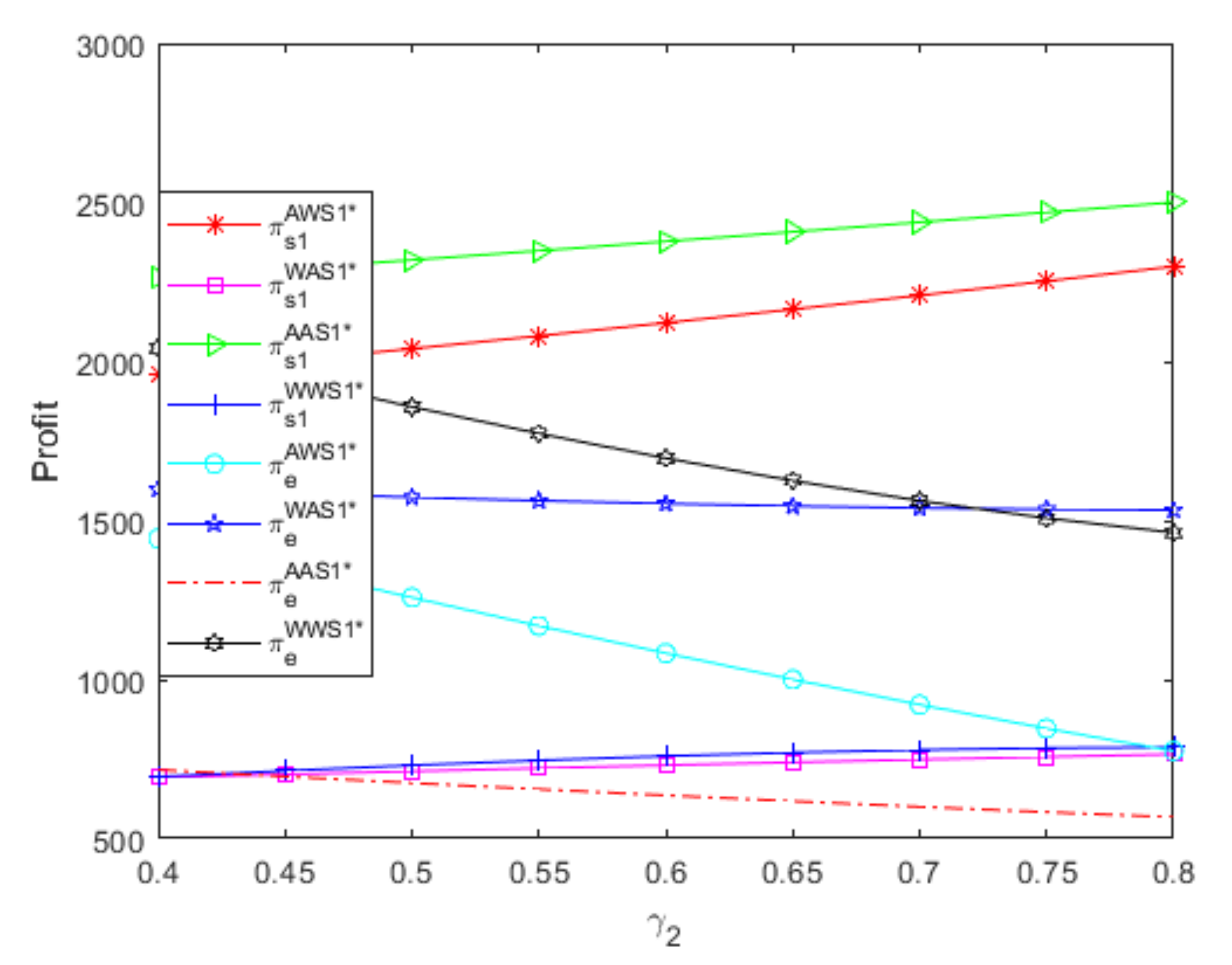
(4.1) 

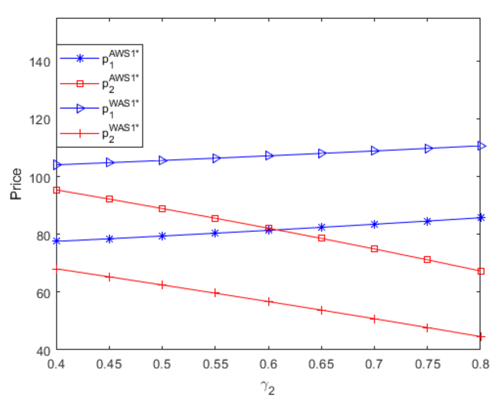
From Figure 4 and Figure 5, when two suppliers use different distribution contracts to sell goods with different levels of complementarity, the optimal retail price of low-complementarity good produced by the powerful supplier is larger than that of high-complementarity good produced by the small supplier only if the two goods’ differences in the level of complementarity are large enough, and the powerful supplier obtains more profits than the small supplier. If the complementarity of good 1 is greater than that of good 2, we can obtain similar results; namely, when two suppliers use different distribution contracts, only if two goods’ differences in the level of complementarity are large enough, the optimal retail price of the low-complementaritygood produced by the small supplier is greater than that of the high-complementarity good producedby the powerful supplier,and the small supplier obtains bigger profits than the powerful supplier.

To limit the number of figures, when two suppliers use different distribution contracts, figures regarding optimal prices and profits if the complementarity of good 1 is greater than that of good 2 are not shown in this article. Thus, when two suppliers use different distribution contracts to sell goods with different levels of complementarity, low-complementarity goods have a greater optimal retail price only if two goods’ differences in the level of complementarity are large enough, and the supplierthat produces goods with lower complementarity obtains more profits regardless ofits distribution contract and channel role.

(4.2) 

If two suppliers use the same distribution contract to sell goods with different levels of complementarity, although the optimal retail/wholesale price of the low-complementarity good produced by the powerful supplier is greater than that of the high-complementarity good produced by the small supplier, the maximum demand of low-complementarity good produced by the powerful supplier is also larger than that of high-complementarity good produced by the small supplier, which leads to that the powerful supplier that produces low-complementarity goods always benefits more than the small supplier that produces high-complementarity goods. These results are valid regardless of two goods’ differences in the level of complementarity.

Discussion 5. 

When two suppliers sell goods with different levels of complementarity, if one supplier uses an A or W contract, we analyze how the goods’ differences in level of complementarity and the other supplier’s distribution contract affect the other supplier’s profit, and draw the following conclusions from Figure 5 and Figure 6.

(5.1) 

From Figure 5, regardless of the distribution contract of the powerful supplierthat produces goods with lower complementarity, two goods’ differences in the level of complementarity have greater negative influences on the small supplier’s profit when it uses an A contract than when it uses a W contract, and the A contract is always more profitable than the W contract for the small supplier that produces high-complementarity goods, which results in that A contract’s advantage decreases as two goods’ differences in the level of complementarity increase. Thus, regardless of the distribution contract of the powerful supplier that produces low-complementarity goods, the small supplier that produces high-complementarity goods always prefers an A contract, and the A contract’s advantage is greater when two goods’ differences in the level of complementarity are relatively low than when two goods’ differences in the level of complementarity are relatively high.

(5.2) 

From Figure 6, no matter what distribution contract the small supplier that produces high-complementarity goods uses, the two goods’ differences in the level of complementarity have greater positive influences on the powerful supplier’s profit when it uses an A contract than when it uses a W contract, and the powerful supplier that produces low-complementarity goods benefits more from an A contract than from a W contract, which leads to that A contract’s advantage increases as two goods’ differences in the level of complementarity increase. Thus, no matter what distribution contract the small supplier that produces high-complementarity goods uses, the powerful supplier that produces low-complementarity goods always prefers the A contract, and the A contract’s advantage is greater when two goods’ differences in the level of complementarity are relatively high than when two goods’ differences in the level of complementarity are relatively low.

Discussion 6. 

When two suppliers sell goods with different levels of complementarity, we study how the differences in the level of complementarity and the two suppliers’ distribution contracts affect the e-retailer’s profit, and derive the results from Figure 6.

If the powerful supplier produces low-complementarity goods and uses a W contract, the e-retailer’s best choice is to let the small supplier do the same when two goods’ differences in the level of complementarity are relatively low, but its best choice is to let the small supplier use an A contract when two goods’ differences in the level of complementarity are relatively high.

(6.1) 

If the powerful supplier produces low-complementarity goods and uses an A contract, two goods’ differences in the level of complementarity have greater negative influences on the e-retailer’s profit when the small supplier uses a W contract than when the small supplier uses an A contract, and the small supplier’s W contract is more profitable for the e-retailer than the small supplier’s A contract, which leads to that W contract’s advantage decreases as two goods’ differences in the level of complementarity increase. Thus, if the powerful supplier produces low-complementarity goods and uses the A contract, the e-retailer should attract the small supplier to use the W contract, and the W contract’s advantage is greater when two goods’ differences in the level of complementarity are relatively low than when two goods’ differences in the level of complementarity are relatively high.

(6.2) 

No matter what contract the small supplier that produces high-complementarity goods uses, two goods’ differences in the level of complementarity have larger negative impacts on the e-retailer’s profit when the powerful supplier uses the A contract than when the powerful supplier uses the W contract, and the powerful supplier’s W contract is more beneficial to the e-retailer than the powerful supplier’s A contract, which results in that W contract’s advantage increases as two goods’ differences in the level of complementarity increase. Therefore, regardless of the distribution contract of the small supplier that produces high-complementarity goods, the e-retailer should attract the powerful supplier to use the W contract, and the W contract’s advantage is larger when two goods’ differences in the level of complementarity are relatively high than when two goods’ differences in the level of complementarity are relatively low.

(6.3) 

If two suppliers use different distribution contracts to sell goods with different levels of complementarity, two goods’ differences in the level of complementarity have larger negative effects on the e-retailer’s profit when the powerful supplier uses the A contract and the small supplier uses the W contract than when the powerful supplier uses the W contract and the small supplier uses the A contract, and the e-retailer obtains more profits when the powerful supplier uses the W contract and the small supplier uses the A contract than when the powerful supplier uses the A contract and the small supplier uses the W contract.

(6.4) 

If two suppliers use the same distribution contract to sell goods with different levels of complementarity, two goods’ differences in the level of complementarity have greater negative influences on the e-retailer’s profit when the two suppliers use the W contract than when the two suppliers use the A contract, and the two suppliers’ W contracts are more beneficial to the e-retailer than the two suppliers’ A contracts, which results in a situation where the W contract’s advantage is greater when two goods’ differences in the level of complementarity are relatively low than when two goods’ differences in the level of complementarity are relatively high.

4.3. Impact of Two Goods’ Differences in the Potential Demand

In this subsection, we investigate how two goods’ differences in the potential demand affect SC members’ decisions and profits. We set $a_1=150$ and take values of $a_2$ from 160 to 260 to characterize two goods’ differences in the potential demand, and the two goods’ differences in the potential demand increase as the parameter $a_2$ increases. The scenario $a_2>a_1$ means that the potential demand of good 2 is greater than that of good 1; thus, good 2 is a called high-demand good, and good 1 is called a low-demand good. We assume the other parameters’ default values are $\varphi =0.10,$ ${\gamma }_1={\gamma }_2=0.3,$ $c_1=c_2=25$, and express the results in Figure 7, Figure 8 and Figure 9.

Discussion 7. 

Two suppliers use the same or different distribution contracts to sell complementary goods with different potential demands on the common e-retailer’s e-platform. When two suppliers use different distribution contracts, we show the results in Figure 7 and Figure 8. To limit the number of figures, when two suppliers use the same distribution contract, we do not present the corresponding results in this article.

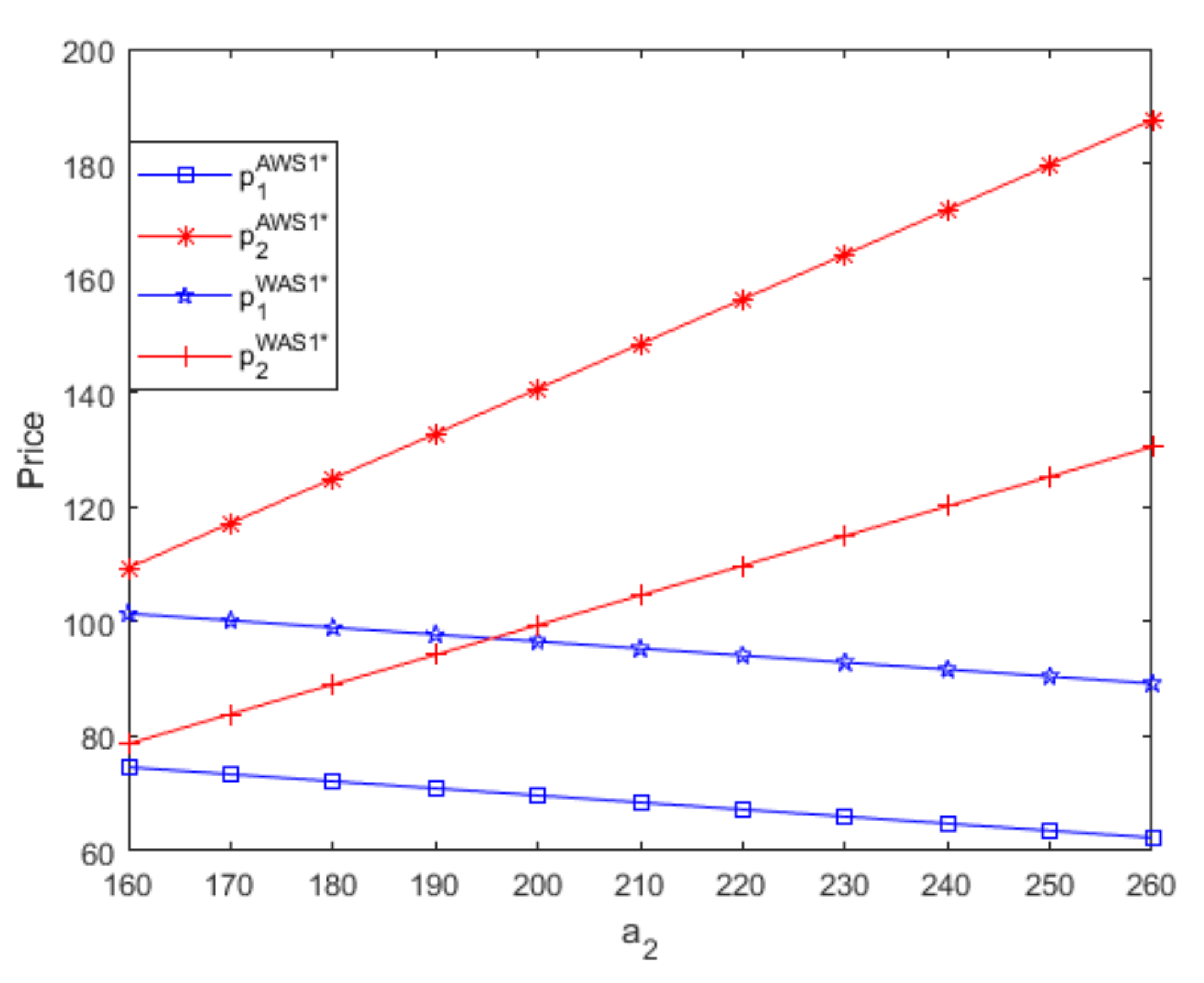
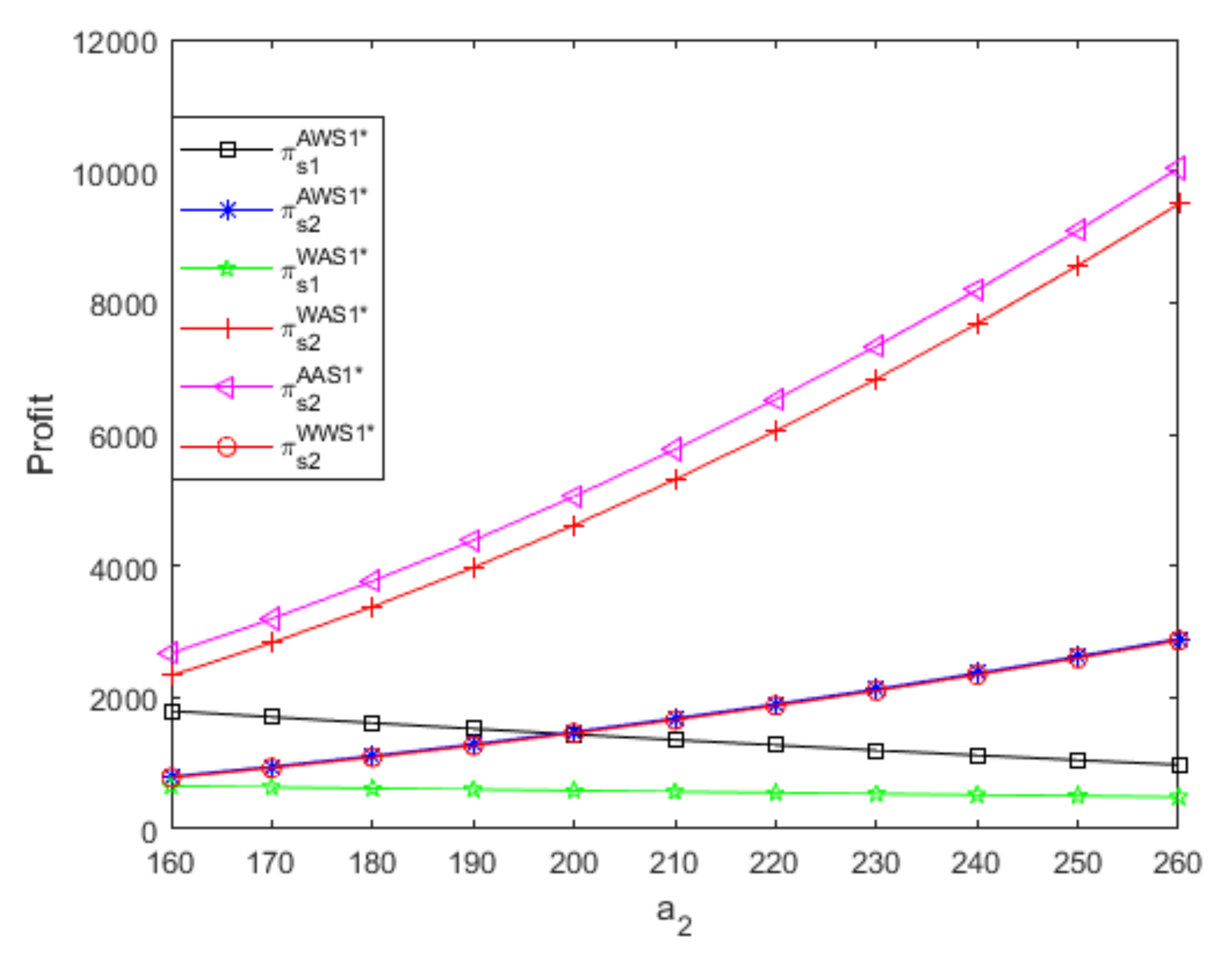
(7.1) 

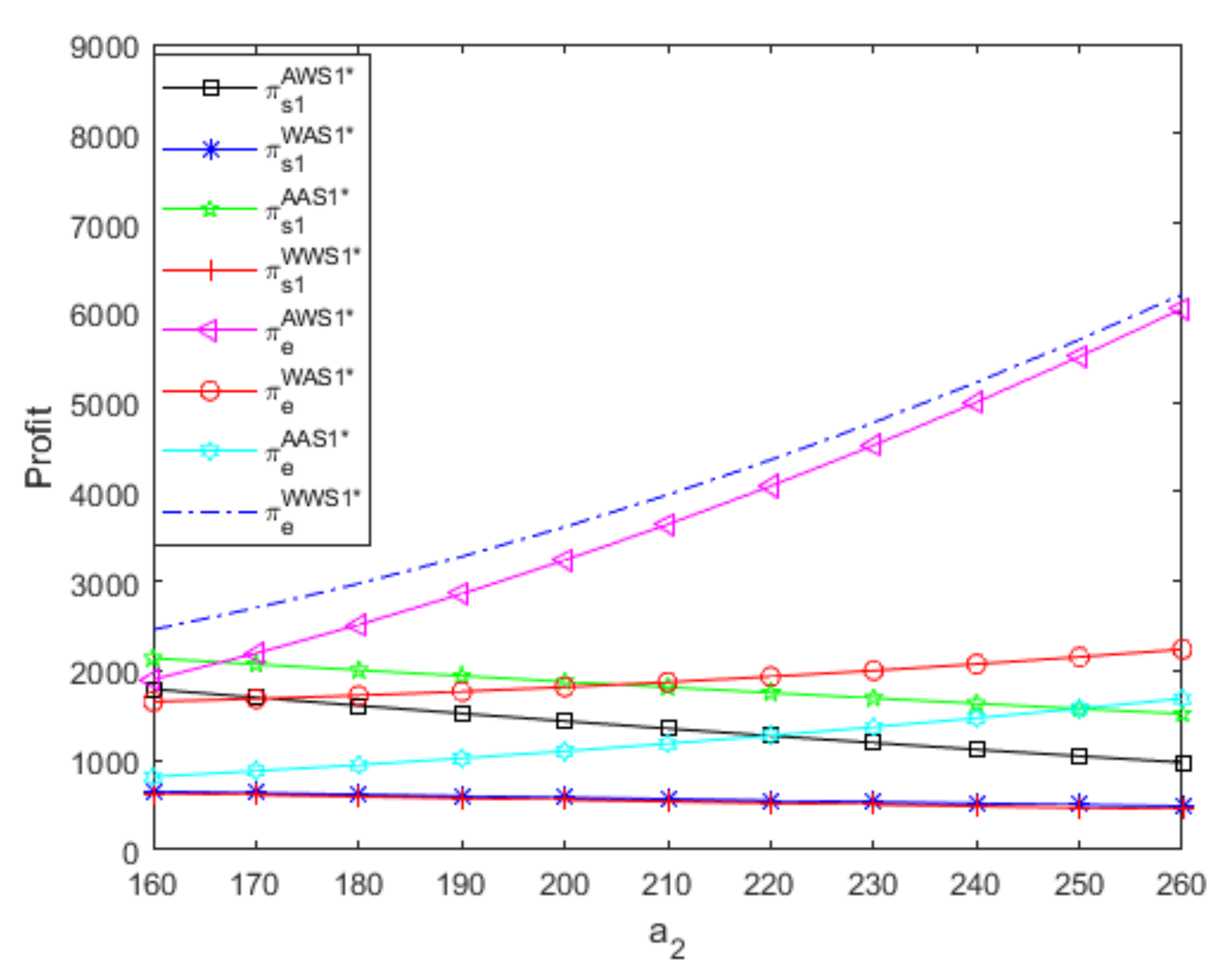
Figure 7 and Figure 8 show that, when two suppliers use different distribution contracts to sell complementary goods with different potential demands, the optimal retail price of high-demand good produced by the small supplier is greater than that of low-demand good produced by the powerful supplier only if the goods’ differences in potential demand are large enough, and the small supplier achieves bigger profits than the powerful supplier. If the potential demand of good 1 is greater than that of good 2, similar results appear; namely, when two suppliers use different distribution contracts, the optimal retail price of high-demand good produced by the powerful supplier is larger than that of low-demand good produced by the small supplier only if two goods’ differences in the potential demand are large enough, and the powerful supplier obtains more profits than the small supplier. For brevity, when two suppliers use different distribution contracts, figures regarding optimal prices and profits if the potential demand of good 1 is greater than that of good 2 are not presented in this article. Thus, when two suppliers use different distribution contracts to sell complementary goods with different potential demands, the high-demand good has a greater optimal retail price only if the goods’ differences in potential demand are large enough, and the supplier that produces high-demand goods obtains more profits regardless of its distribution contract and channel role

(7.2)  

Regardless of two goods’ differences in the potential demand, when two suppliers use the same distribution contract, the high-demand good produced by the small supplier always has a larger optimal wholesale/retail price than low-demand good produced by the powerful supplier, and no matter which distribution contracts the two suppliers both use, the small supplier that produces high-demand goodsalways benefits more than the powerful supplier that produces low-demand goods.

Discussion 8. 

When two suppliers sell complementary goods with different potential demands, if one supplier uses an A or W contract, we explore how the goods’ differences in potential demand and the other supplier’s distribution contract affect the other supplier’s profit, and draw the following conclusions from Figure 8 and Figure 9.

(8.1)  

From Figure 8, no matter what distribution contract the powerful supplier that produces low-demand goods uses, two goods’ differences in the potential demand have greater positive influences on the small supplier’s profit when it uses the A contract than when it uses the W contract, and the A contract is more profitable than the W contract for the small supplier that produces high-demand goods, which leads to that A contract’s advantage increases as the two goods’ differences in the potential demand increase. Thus, regardless of the distribution contract of the powerful supplier that produces low-demand goods, the small supplier that produces high-demand goods should choose the A contract, and the A contract’s advantage is larger when two goods’ differences in the potential demand are relatively high than when two goods’ differences in the potential demand are relatively low.

(8.2)  

As illustrated in Figure 9, no matter what distribution contract the small supplier that produces high-demand goods uses, although two goods’ differences in the potential demand have larger negative effects on the powerful supplier’s profit when it uses the A contract than when it uses the W contract, the A contract is always more profitable than the W contract for the powerful supplier that produces low-demand goods, which results in a situation where the A contract’s advantage decreases as two goods’ differences in the potential demand increase. Thus, regardless of the distribution contract of the small supplier that produces high-demand goods, the powerful supplier that produces low-demand goods should choose the A contract, and the A contract’s advantage is larger when two goods’ differences in the potential demand are relatively low than when two goods’ differences in the potential demand are relatively high.

Discussion 9. 

When two suppliers sell complementary goods with different potential demands, we study how the goods’ differences in the potential demand and the two suppliers’ distribution contracts affect the e-retailer’s profit, and derive the results from Figure 9.

(9.1) 

Regardless of two suppliers’ distribution contracts and channel roles, the e-retailer’s profit increases as two goods’ differences in the potential demand increase. The e-retailer achieves the maximum profit when two suppliers both use the W contract and achieves the least profit when two suppliers both use the A contract, which is independent of two goods’ differences in the potential demand.

(9.2) 

If two suppliers use different distribution contracts to sell complementary goods with different potential demands, two goods’ differences in the potential demand have greater positive influences on the e-retailer’s profit when the powerful supplier uses A contract and the small supplier uses W contract than when the powerful supplier uses W contract and the small supplier uses the A contract, and the e-retailer obtains more profits when the powerful supplier uses the A contract and the small supplier uses the W contract than when the powerful supplier uses the W contract and the small supplier uses the A contract.

(9.3) 

No matter what distribution contract the small supplier that produces high-demand goods uses, although two goods’ differences in the potential demand have greater positive influences on the e-retailer’s profit when the powerful supplier uses the A contract than when the powerful supplier uses the W contract, the powerful supplier’s W contract is more beneficial to the e-retailer than the powerful supplier’s A contract, which results in a situation where the W contract’s advantage decreases as two goods’ differences in the potential demand increase. Thus, no matter what distribution contract the small supplier that produces high-demand goods uses, the e-retailer should guide the powerful supplier to use the W contract, and the W contract’s advantage is larger when two goods’ differences in the potential demand are relatively low than when two goods’ differences in the potential demand are relatively high.

(9.4) 

Regardless of the distribution contract of the powerful supplier that produces low-demand goods, two goods’ differences in the potential demand have greater positive influences on the e-retailer’s profit when the small supplier uses the W contract than when the small supplier uses the A contract, and the small supplier’s W contract is more profitable for the e-retailer than the small supplier’s A contract, which leads to that the W contract’s advantage increases as two goods’ differences in the potential demand increase. Thus, regardless of the distribution contract of the powerful supplier that produces low-demand goods, the e-retailer should guide the small supplier to use the W contract, and the W contract’s advantage is greater when two goods’ differences in the potential demand are relatively high than when two goods’ differences in the potential demand are relatively low.

5. Conclusions

This paper explores the interaction between two suppliers’ distribution contract choices on the same e-retailer’s e-platform and their channel roles. Specifically, this paper focuses on an SC including an e-retailer that is the SC leader, and two suppliers that are the SC followers. Each supplier produces a good and sells it on the e-retailer’s e-platform, and the two goods are functionally complementary. The e-retailer provides each supplier with two contracts (A and W contracts). Moreover, different suppliers differ in their channel roles, and this paper assumes supplier 1 is the channel leader and supplier 2 is the channel follower.

By comparing and analyzing equilibrium solutions of four game models and exploring the impact of some key factors on SC members’ decisions and profits, we provide some management implications for SC members. For the e-retailer, when two suppliers sell goods with different levels of complementarity on the e-retailer’s online platform, if the powerful supplier produces low-complementarity goods and adopts the W contract, the e-retailer should attempt to induce the small supplier to adopt the W contract when two goods’ differences in the level of complementarity are relatively low, while the opposite result appears when two goods’ differences in the level of complementarity are relatively high. Moreover, when two suppliers sell complementary goods with symmetric parameters on the common e-retailer’s online platform, regardless of one supplier’s distribution contract, the e-retailer should attempt to attract the other supplier to use the W contract, and the W contract’s advantage is greater when the referral fees are relatively low than when the referral fees are relatively high.

For two suppliers, no matter what distribution contract one supplier uses, the other supplier always should adopt the A contract, which is independent of two suppliers’ channel roles, the e-retailer’s referral fees, two goods’ differences in the level of complementarity and two goods’ differences in the potential demand. If two suppliers use different distribution contracts to sell complementary goods with symmetric parameters, the supplier always benefits more from the A contract than from the W contract regardless of the referral fees and the supplier’s channel role. Moreover, when two suppliers use different distribution contracts to sell two complementary goods with different potential demands, the high-demand good has a larger optimal retail price only if two goods’ differences in the potential demand are sufficiently high, and producing the high-demand good makes the supplier obtain more profits regardless of the supplier’s distribution contract and channel role.

This paper has several limitations which provide possible directions to extend this study. First, this paper addresses our research questions with linear and deterministic demand functions, and it would be interesting to study whether our results are still valid with nonlinear and stochastic demand functions. Second, this paper considers only the different channel roles between suppliers in the same echelon; however, the different channel roles between e-retailers in the same echelon also affect SC members’ decisions and profits, and conducting our research in an SC with multiple e-retailers that have different channel roles is meaningful. Finally, this paper assumes all SC members are information-complete; nevertheless, the e-retailer can use big data technology to gather massive amounts of information from the e-platform, and the information sharing between SC members is worth studying in the future.

References

- Abhishek, V.; Jerath, K.; Zhang, Z.J. Agency selling or reselling? Channel structures in electronic retailing. Manag. Sci. 2016, 62, 2259–2280. [Google Scholar] [CrossRef] [Green Version]
- Lu, Q.; Shi, V.; Huang, J. Who benefit from agency model: A strategic analysis of pricing models in distribution channels of physical books and e-books. Eur. J. Oper. Res. 2018, 264, 1074–1091. [Google Scholar] [CrossRef]
- Yan, Y.; Zhao, R.; Xing, T. Strategic introduction of the marketplace channel under dual upstream disadvantages in sales efficiency and demand information. Eur. J. Oper. Res. 2019, 273, 968–982. [Google Scholar] [CrossRef]
- Geng, X.; Tan, Y.; Wei, L. How add-on pricing interacts with distribution contracts. Prod. Oper. Manag. 2018, 27, 605–623. [Google Scholar] [CrossRef]
- Tian, L.; Vakharia, A.J.; Tan, Y.; Xu, Y. Marketplace, reseller, or hybrid: Strategic analysis of an emerging e-commerce model. Prod. Oper. Manag. 2018, 27, 1595–1610. [Google Scholar] [CrossRef]
- Yan, Y.; Zhao, R.; Liu, Z. Strategic introduction of the marketplace channel under spillovers from online to offline sales. Eur. J. Oper. Res. 2018, 267, 65–77. [Google Scholar] [CrossRef]
- Zhang, S.; Zhang, J. Agency selling or reselling: E-tailer information sharing with supplier offline entry. Eur. J. Oper. Res. 2020, 280, 134–151. [Google Scholar] [CrossRef]
- EI-Ansary, A.L.E.; Stern, L.W. Power measurement in the distribution channel. J. Mark. Res. 1972, 9, 47–52. [Google Scholar] [CrossRef]
- Shi, R.; Zhang, J.; Ru, J. Impacts of power structure on supply chains with uncertain demand. Prod. Oper. Manag. 2013, 22, 1232–1249. [Google Scholar] [CrossRef]
- Wei, J.; Zhao, J.; Li, Y. Pricing decisions for complementary products with firms’ different market powers. Eur. J. Oper. Res. 2013, 224, 507–519. [Google Scholar] [CrossRef]
- Luo, Z.; Chen, X.; Chen, J.; Wang, X. Optimal pricing policies for differentiated brands under different supply chain power structures. Eur. J. Oper. Res. 2017, 259, 437–451. [Google Scholar] [CrossRef] [Green Version]
- Li, T.; Zhang, R.; Liu, B. Pricing decisions of competing supply chains under power imbalance structures. Comput. Ind. Eng. 2018, 125, 695–707. [Google Scholar] [CrossRef]
- Mukhopadhyay, S.K.; Yue, X.; Zhu, X. A Stackelberg model of pricing of complementary goods under information asymmetry. Int. J. Prod. Econ. 2011, 134, 424–433. [Google Scholar] [CrossRef]
- Wang, J.; Yan, Y.; Du, H.; Zhao, R. The optimal sales format for green products considering downstream investment. Int. J. Prod. Res. 2020, 58, 1107–1126. [Google Scholar] [CrossRef]
- Wei, J.; Lu, J.; Wang, Y. How to Choose Online Sales Formats for Competitive E-Tailers, International Transactions in Operational Research. Available online: https://0-doi-org.brum.beds.ac.uk/10.1111/itor.12777 (accessed on 1 January 2020).
- Zennyo, Y. Strategic contracting and hybrid use of agency and wholesale contracts in e-commerce platforms. Eur. J. Oper. Res. 2020, 281, 231–239. [Google Scholar] [CrossRef]
- Tan, Y.; Carrillo, J.E. Strategic analysis of the agency model for digital goods. Prod. Oper. Manag. 2017, 26, 724–741. [Google Scholar] [CrossRef]
- Wei, J.; Zhao, J.; Hou, X. Bilateral information sharing in two supply chains with complementary products. Appl. Math. Model. 2019, 72, 28–49. [Google Scholar] [CrossRef]
- Yue, X.; Mukhopadhyay, S.K.; Zhu, X. A Bertrand model of pricing of complementary goods under information asymmetry. J. Bus. Res. 2006, 59, 1182–1192. [Google Scholar] [CrossRef]
- Karray, S.; Sigue, S.P. Should companies jointly promote their complementary products when they compete in other product categories? Eur. J. Oper. Res. 2016, 255, 620–630. [Google Scholar] [CrossRef]
- Sinitsyn, M. Coordination of price promotions in complementary categories. Manag. Sci. 2012, 58, 2076–2094. [Google Scholar] [CrossRef]
- He, Y.; Yin, S. Joint selling of complementary components under brand and retail competition. Manuf. Serv. Oper. Manag. 2015, 17, 470–479. [Google Scholar] [CrossRef] [Green Version]
- Wang, Y. Joint pricing-production decisions in supply chains of complementary products with uncertain demand. Oper. Res. 2006, 54, 1110–1127. [Google Scholar] [CrossRef]
- Yin, S. Alliance formation among perfectly complementary suppliers in a price-sensitive assembly system. Manuf. Serv. Oper. Manag. 2010, 12, 527–544. [Google Scholar] [CrossRef]
- Jalali, H.; Ansaripoor, A.H.; Giovanni, P.D. Closed-loop supply chains with complementary products. Int. J. Prod. Econ. 2020, 229, 107757. [Google Scholar] [CrossRef]
- Lan, Y.; Cai, X.; Shang, C.; Zhang, L.; Zhao, R. Heterogeneous suppliers’ contract design in assembly systems with asymmetric information. Eur. J. Oper. Res. 2020, 286, 149–163. [Google Scholar] [CrossRef]
- Ren, D.; Lan, Y.; Shang, C.; Wang, J.; Xue, C. Impact of trade credit on pricing decisions of complementary products. Comput. Ind. Eng. 2020, 146, 106580. [Google Scholar] [CrossRef]
- Wang, L.; Song, H.; Wang, Y. Pricing and service decisions of complementary products in a dual-channel supply chain. Comput. Ind. Eng. 2017, 105, 223–233. [Google Scholar] [CrossRef]
- Li, F.; Li, S.; Gu, J. Whether to delay the release of eBooks or not? An analysis of optimal publishing strategies for book publishers. J. Theor. Appl. Electron. Commer. Res. 2019, 14, 124–137. [Google Scholar] [CrossRef] [Green Version]
- Lou, Y.; He, Z.; Feng, L.; Cai, k.; He, S. Original Design Manufacturer’s Warranty Strategy When Considering Retailers’ Brand Power Under Different Power Structures, International Transactions in Operational Research. Available online: https://0-doi-org.brum.beds.ac.uk/10.1111/itor.12795 (accessed on 1 April 2020).
- Wang, J.; Wang, Y.; Lai, F. Impact of power structure on supply chain performance and consumer surplus. Int. Trans. Oper. Res. 2019, 26, 1752–1785. [Google Scholar] [CrossRef]
- Tsay, A.A.; Agrawal, N. Channel dynamics under price and service competition. Manuf. Serv. Oper. Manag. 2000, 2, 372–391. [Google Scholar] [CrossRef]
- Chen, L.; Tang, W. Analysis of network effect in the competition of self-publishing market. J. Theor. Appl. Electron. Commer. Res. 2020, 15, 50–68. [Google Scholar] [CrossRef]
- Mishra, B.K.; Raghunathan, S. Retailer- vs. vendor-managed inventory and brand competition. Manag. Sci. 2004, 50, 445–457. [Google Scholar] [CrossRef] [Green Version]