Dynamic Marketing Resource Allocation with Two-Stage Decisions

Abstract

In the precision marketing of a new product, it is a challenge to allocate limited resources to the target customer groups with different characteristics. We presented a framework using the distance-based algorithm, K-nearest neighbors, and support vector machine to capture customers’ preferences toward promotion channels. Additionally, online learning programming was combined with machine learning strategies to fit a dynamic environment, evaluating its performance through a parsimonious model of minimum regret. A resource optimization model was proposed using classification results as input. In particular, we collected data from an institution that provides financial credit products to capital-constrained small businesses. Our sample contained 525,919 customers who will be introduced to a new product. By simulating different scenarios between resources and demand, we showed an up to 22.42% increase in the number of expected borrowers when KNN was performed with an optimal resource allocation strategy. Our results also show that KNN is the most stable method to perform classification and that the distance-based algorithm has the most efficient adoption with online learning.

1. Introduction

Marketing resource allocation has been a topic of intense scrutiny, yet the literature on the topic has not paid adequate attention to the fact that the effectiveness of marketing-mix elements varies over time [1]. Despite the fact that firms collect volumes of data on their customers, existing estimation approaches do not readily lend themselves to modeling their data and provide little guidance to companies in terms of their resource allocation decision. Firms have long been concerned with optimizing the allocation of their limited resources across multiple marketing activities. As a result of the limited marketing budget, marketers must find ways to maximize the impact of their marketing dollars. High-efficiency marketing can capture a large number of potential customers quickly with a rational cost of promotion resources.

One motivation for conducting this research is to understand the relationship between customer features and product features so that we can map customers to the right products. According to Rust et al. [2], customers who have bought a similar product previously are likely to buy the newly launched product. With limited promotion resources, the allocation of different types of resources to receive the maximum number of product buyers/users becomes an issue. For instance, face-to-face marketing is the most effective way for product promotion while it consumes the most resources, which is followed by promotion by phone, promotion through e-mail, or other message channels. Another equally important motivation is that in practice, companies must decide on the amount of resources that they need to allocate to each customer in the coming week or month. However, most academic studies overlook such short-term decisions. The third motivation for us to conduct this study is that when launching new products, it is famously difficult to forecast their accurate marketing demand. That is, it is quite challenging to have a clear recognition in customers’ preferences and hence targeting potential customers, because lacking historical sales data makes it rather hard to reveal valuable information about customers’ preferences [3].

To fill the gaps in academic perspective and in practice as mentioned above, we raised the following research questions of this paper.

• What strategies can be utilized to link the customers’ preferences forecasting with capital/resource utilization maximization?
• How can we set a suitable marketing decision period that has the most noteworthy effect on sales?
• What techniques are utilized to forecast marketing demand facing short of historical sales data of new products?

In this research, we classify all potential customers into several types to allocate different resources. In this case, a promotion activity with limited resources under uncertain demand in achieving high promotion effectiveness becomes an optimized problem, i.e., with the largest number of customers buying the new product ultimately.

We present a two-stage framework to deal with decision making in dynamic marketing resource allocation, including customer classification and optimization of resource allocation. To achieve in-time allocation (even within a short time period), we combined online learning by adding marketing feedback into our model.

1.1. Key Results

To illustrate our framework in detail, we presented a case study of a newly launched credit loan product focusing on small businesses. Target customers are seeking short-term funding and sensitive to interest rates. Small businesses have different preferences in product promotion channels, making it suitable for us to analyze the strategy our marketing resource allocation.

Our key results are listed as follows.

• In the first stage of customer classification (targeting customers), we adopted three classic methodologies related to machine learning—distance-based method, K-nearest neighbors (KNN), and support vector machine (SVM)—over multiple heterogeneous features among potential customers. From the perspective of running time, the distance-based method used the shortest time to complete the classification process; KNN was the most stable in terms of predicted accuracy, although it cost twice as much time as that of the distance-based method. SVM showed a slightly higher predicted accuracy than that of the distance-based method, but it took a much long time to do classification due to finding its convex optimization results. Furthermore, as observations made in the training sample were all buyers/users who accepted a product that was very similar to the newly launched product, we had no information about customers who were uninterested in this new product. To deal with this issue, an online learning strategy was proposed. We found that the distance-based algorithm always reached its stable state after one episode, while KNN and SVM had a slower speed when learning.
• In the second stage of optimization of resource allocation, classification results were then taken as input parameters of resource optimization for allocation of resources. Experiments were also conducted to compare the optimal resource allocation with the marketing strategies currently adopted by the loan agency. Our simulation results showed that the higher predicted accuracy one algorithm yields, the greater the increase in final expected buyers/users, thus, the better the allocation proposal. Among the three classification algorithms, KNN outperformed others with a 22.42% increase in final expected customers. With more expected customers wanting to try new products under the scenario of limited promotion resources, the corresponding classification methodology together with optimal resource allocation plan are an improvement toward the promotion strategy that the company adopts at present.

Below, we first review the related literature and highlight our contributions to both the literature and practice in the rest of this section. Then, in Section 2, we describes the proposed framework, including the first stage of customer classification to find their promotion preference and the second stage of resource allocation to optimize capital constrained marketing resources. In Section 3, we apply our approach on a dataset to further implement the theoretical model and evaluate its effectiveness with detailed results.

Section 4 discusses our research results and relates them to existing literature. Finally, Section 5 presents the conclusions, limitations, both managerial and practical implications, and further research directions.

1.2. Literature Review

Our study is related to two streams of literature: one for the literature of the prediction of customers’ preferences, and the other for the optimization of multiple resource allocation under a capital constrained circumstance.

The marketing strategy of how to target customers across various promotion channels is becoming a critical issue in practice [4]. A number of works in precision marketing study product promotion by recognizing customers’ preferences to understand and forecast future purchase behavior. For example, some researchers conducted analytics through data and found that personalized promotion can have an influence on customer retention and sales [5,6,7]. For instance, focusing on mobile marketing effects, some researchers applied field data to explore optimal effects with customer location and weather [8,9,10,11]. Malthouse and Derenthal [12] proposed aggregated scoring models by developing averaging predictions to target the right customers. Li et al. [13] proposed a lifecycle forecast approach to predict product demand in each period. Kumar et al. [14] conducted their study to investigate the contributions of the promotion marketing strategy to customers demand using fuzzy neural network. He et al. [15] designed estimated preference parameters to study customer demand in the station network of the London bike-share system. Some focused on multichannel marketing, and they found that customers who are provided with multiple channels are more profitable to companies than single-channel customers [16,17,18]. Hwang [19] proposed two new approaches in variable selection to deal with collaborative filtering as well as target marketing. However, a limited marketing budget indicates that targeting customers through multiple channels is usually unrealistic.

To deal with a fixed marketing budget, a more specific area of interest within this broader space is studying how to allocate the limited budget to several promotion activities. Perdikaki et al. [20] proposed an optimization centralized model for budget allocation between store labor and marketing activities such as advertising with the objective of maximizing store sales. Ban and Rudin [21] studied a newsvendor decision-maker to make a sensible ordering decision according to past information about various features of the demand. Further investigation showed that their custom-designed, feature-based algorithms yielded substantially lower cost than several main benchmarks known in the literature. Luzon et al. [22] examined the dynamic allocation of budget for an online advertisement campaign posted through a social network. They considered unique features of social network marketing and aimed at minimizing the campaign’s length upon reaching a desired level of exposure of each marketing segment. Memarpour et al. [23] used the Markov decision process with a budget constraint and measured customers’ profitability through customer equity to find the optimal allocation strategy. Previous studies focused on marketing resources related to budget decisions indicated that profit improvement from better allocation across products or regions is much higher than that from improving the overall budget [24]. Koosha and Albadvi [25] provided a multi-period process model to allocate marketing budget to customer segments in a long-term view and a dynamic process. Genetic algorithm and simulated annealing approaches were adopted to find the near optimal solution. In fact, heuristic methods are usually used by marketing practitioners to determine the marketing budget, although a small amount of research has studied budget questions [26]. They focused on optimizing the budget for a product in a static environment, while we tried to solve the allocation problem under the consideration of uncertain market demand, i.e., the dynamic preference of customers. In the research of resource allocation, it has been pointed out that resource allocations based on historical performance can be counter-productive and that marketing managers should continuously reallocate marketing resources based on the expected returns [27].

Some studies explore how to solve the resource allocation problems under multiple channels in a specific industry. For example, Salmani and Partovi [28] proposed a resource allocation matric to measure the value of channel structure within multiple channels iin the retailing industry. Li et al. [29] develop a two-category two-period model considering network effects and cross-category interdependence to find optimal resource allocation strategies in platform businesses. Our research differs from those in that we propose a general framework to solve the dynamic marketing resource allocation problem, which can be adopted in different scenarios and is not restricted to industries.

Compared with the existing literature, the contributions of our research to both the literature and practice lie in the following aspects.

• Our research constructed a cost-effective solution through integrating the forecasting of preferences toward the promotion channel and the optimization of resource allocation, rather than solving them separately as typically performed.
• We derive a theoretical relationship between the preference probability and the optimization of a limited marketing budget.
• Academic studies overlook short-term decisions, while our proposed framework is flexible and can analyze in time to help making marketing decisions.
• Current forecast methods use sufficient sales data to predict a mid-range lifecycle. However, we generate practical steps for obtaining an accurate early lifecycle forecast.
• We conducted an online convex programming algorithm to analyze customers with no interest in the new product.
• We proposed a framework that can be adopted in different scenarios and is not restricted to industries.

2. Materials and Methods

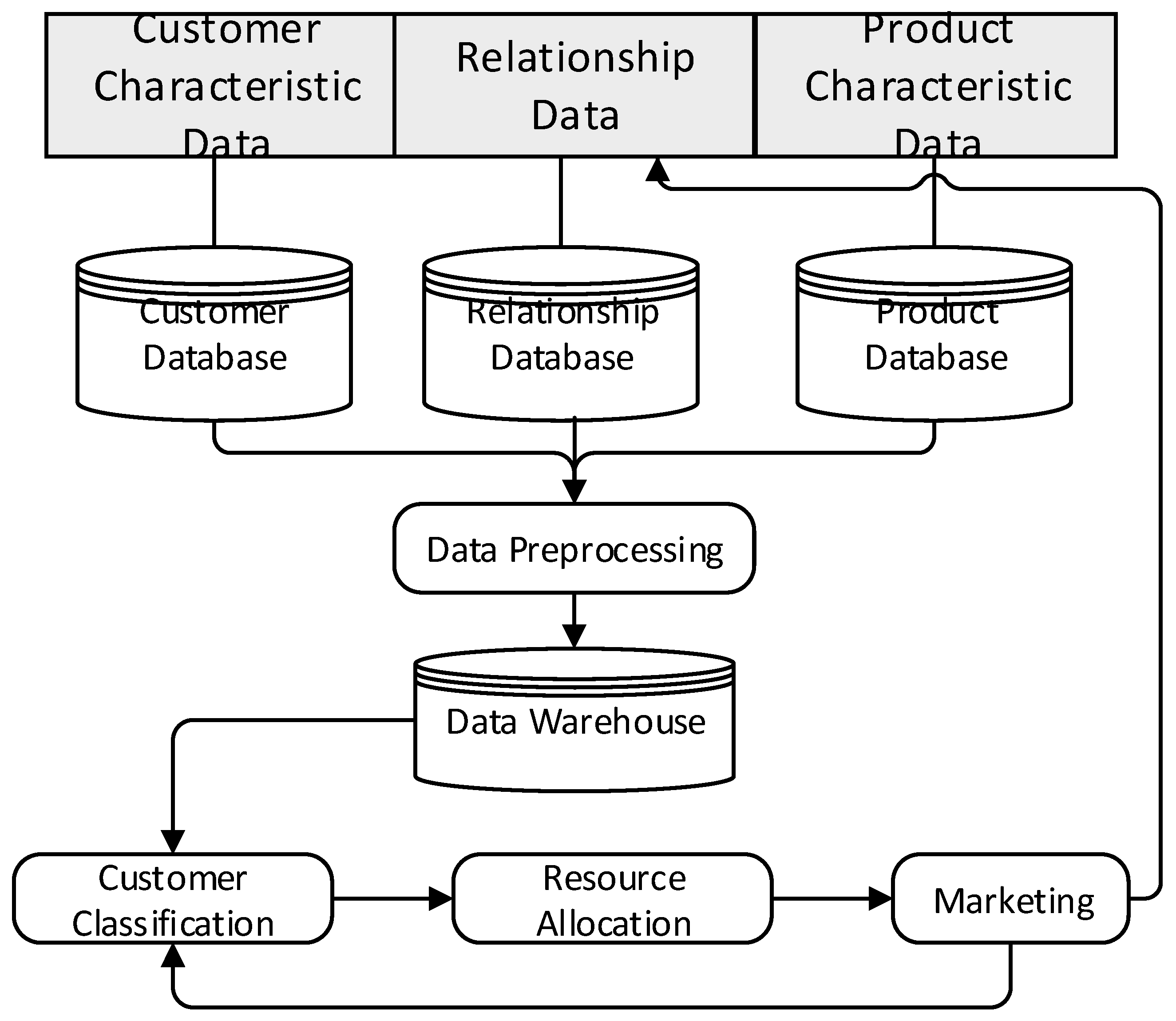
This section describes the methodology employed in our research. The main process of precision marketing relies on the relationship between customers and products, upon which we establish a data warehouse. The data layer consists of three databases (customer database, product database, and relationship database), and it is responsible for receiving real-time data, preprocessing it, as well as loading the data warehouse for the next layer of data analysis. The analysis layer includes customer classification and resource allocation, which are the core of the entire marketing strategy. Our classification methodology includes a distance-based algorithm, KNN, and SVM to identify the preference of customers toward the promotion channel. Resource allocation uses optimization models to formulate the relationship between customer demand and limited resources. We tested customers belonging to 8 distributions separately without loss of generality. The analysis layer provides marketing solutions for the decision-making layer, and it also obtains feedback from the decision-making layer for adjustment. The decision-making layer uses strategies generated from the analysis layer to return feedback to both the data layer and analysis layer. Figure 1 illustrates our framework to implement precision marketing.

2.1. Customer Classification

In this part, we present the classification algorithms used in our research. Defining customers in the training set as $S_1,s_iϵS_1,i=1,\cdots m$, and potential customers as $S_2,s_jϵS_2,j=1,\cdots ,n$, we standardize two samples and modeling according to the different scenarios below.

To analyze how to target customers, we first present the situation in which the promotion channel is unknown. Denote central point $s_c$ among training customers as $s_c=\frac{1}{m}{\sum }_{i=1}^m{s}_i$. We formulate distance $d_j$ between a potential customer $s_j$ and $s_c$ as $d_j=\sqrt{{(s_j-s_c)}^2}$. Customers with smaller distance are more likely to belong to the same class. In terms of resource allocation, we consider that closer customers should be first promoted. With only one type of resource, allocate all resources to customers with the minimum distance; when several types of resources exist, allocate different types of resources to customers according to the distance with the stronger promotion efficiency given to the closer customer, for example, face-to-face promotion, followed by promotion by phone, then e-mail or message.

Next, we study the scenario when the promotion channel is known and there are several types of promotion resources. We present three methods for supervised learning: distance-based method, KNN, and SVM. Resource allocation strategies will be introduced later on.

2.1.1. Distance-Based Method

Based on the Euclidean distance, customer classification through a distance-based algorithm could quickly identify the class a customer belongs to. Labels in the training set indicate the promotion preference of customers. We split training set $S_1$ into p subset with $S_k$ representing the kth class. Given $s_{ck}$ of the kth class as an example, denote central points of each class, as

$$s_{ck}=\frac{1}{m}\sum _{i\in S_k}{s}_i,S_k\subset S_1$$

(1)

where m represents the number of customers in class k. We assign a class label with a minimum distance to customers, taking class $y_j\left(k\right)$ of customer j as an example,

$$y_j\left(k\right)=\underset{k=1,...,p}{argmin}\sqrt{{(s_j-s_{ck})}^2}$$

(2)

2.1.2. K-Nearest Neighbors

The classification through KNN resets sample variables into $(X,Y)$, with X describing customer characteristics such as age and Y stands for the label of promotion channel such as face-to-face. As the exact conditional distribution of Y given X is unknown, perform classification according to K customers in the training sample who are closest to the potential customer, and consider the highest probability of which class the potential customer belongs to on the basis of which class the K customers are in.

We provide a mathematical description with reference to James [30]. Given positive integer K and one potential customer $x_0$, the KNN classifier identifies the K customers that are closest to $x_0$, represented by $N_0$. Then, KNN estimates the conditional probability for class j as the fraction of points in $N_0$ whose class label equals j:

$$Pr(Y=j|X=x_0)=\frac{1}{K}\sum _{i\in N_0}I(y_i=j)$$

(3)

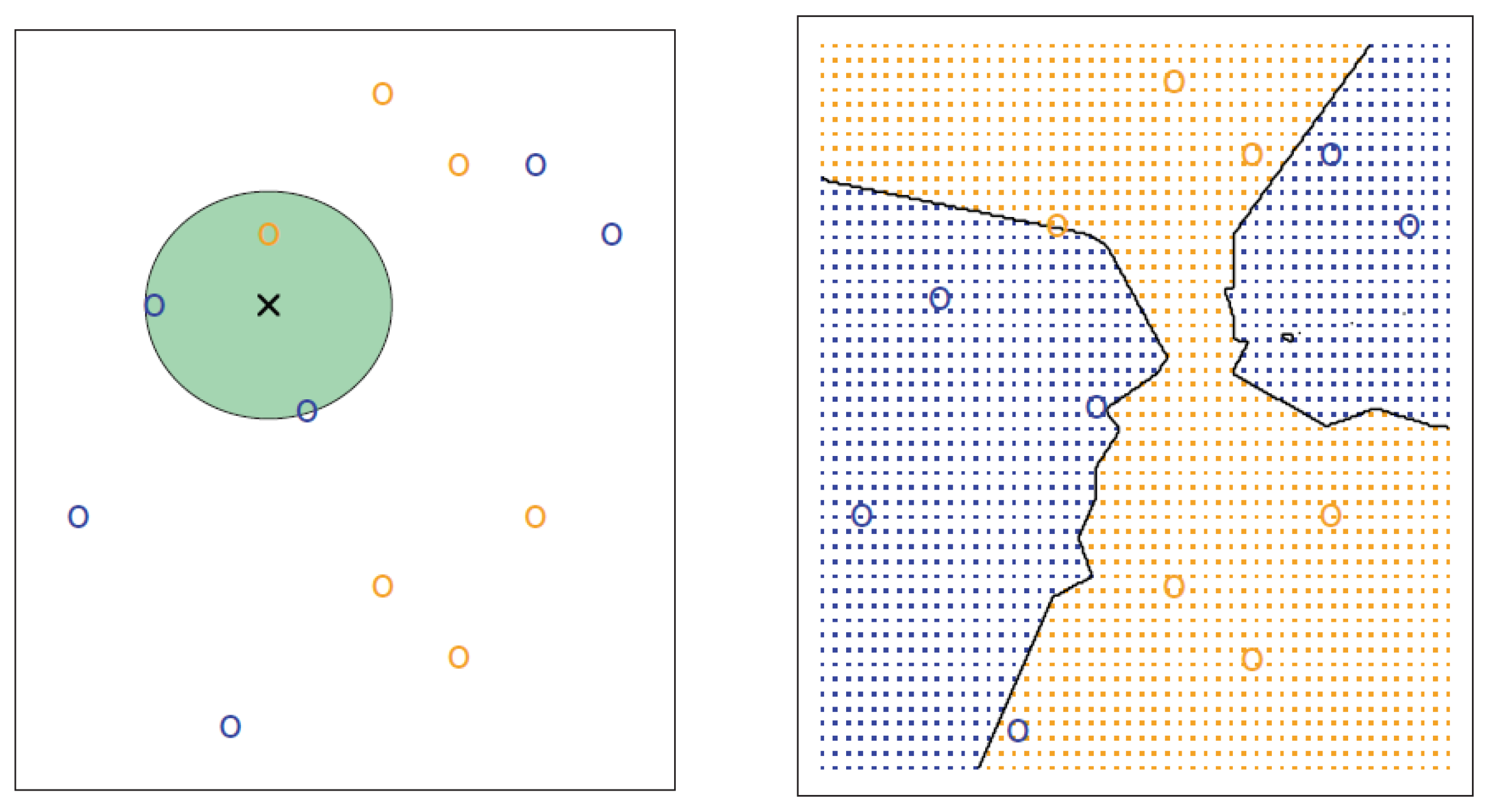
KNN applies the Bayes rule and classifies potential customer $x_0$ to the class with the largest probability. As to the selection of K, cross-validation is considered the most common method. To further explain KNN, we present a simple situation with six blue observations and six orange observations, as shown in Figure 2, with $K=3$. The left shows a test observation at which a predicted class label is depicted as a black cross. The three closest points to the test observation are identified, and it is predicted that the test observation belongs to the most commonly occurring class, i.e., blue in this case. The right shows the KNN decision boundary for this example in black. The blue grid indicates the region in which a test observation will be assigned to the blue class, and the orange grid indicates the region in which it will be assigned to the orange class.

2.1.3. Support Vector Machine

Support vector machine (SVM) is a special case of support vector classifier, an extension resulting from enlarging feature space in a specific way, using kernels. Take n training customers for example:

$$({\overrightarrow{x}}_1,y_1),\cdots ({\overrightarrow{x}}_n,y_n)$$

where ${\overrightarrow{x}}_i$, a vector in p-dimensional space, describes customer characteristics such as gender while $y_i=-1$ or $y_i=1$, representing the promotion preference of ${\overrightarrow{x}}_i$. SVM aims at splitting all the observations of $y_i=1$ and $y_i=-1$ by a “maximum margin hyperplane”, which is defined so that the distance between the hyperplane and the nearest point ${\overrightarrow{x}}_i$ from either group is maximized.

For a certain hyperplane, $\overrightarrow{x}$ in that space must satisfy the following constraint:

$$\overrightarrow{\omega }·\overrightarrow{x}-b=0$$

(4)

where $\overrightarrow{\omega }$ is the normal vector (not necessarily normalized) to the hyperplane and parameter $\frac{b}{∥\overrightarrow{\omega }∥}$ determines the offset from the hyperplane toward $\overrightarrow{\omega }$. We classify a potential customer based on which side of the maximal margin hyperplane it lies. To extend SVM to cases in which data are not linearly separable, we introduce the hinge loss function:

$$max(0,1-y_i(\overrightarrow{\omega }·{\overrightarrow{x}}_i-b))$$

(5)

When the constraint above is satisfied, the function is zero, which indicates that ${\overrightarrow{x}}_i$ lies on the correct side of the margin. For data on the wrong side, the value of the function is proportional to the distance from the margin. Then, we hope to minimize

$$[\frac{1}{n}\sum _{i=1}^{n}max(0,1-y_i(\overrightarrow{\omega }·{\overrightarrow{x}}_i-b))]+\lambda {(∥\overrightarrow{\omega }∥)}^2]$$

(6)

where the parameter $\lambda$ determines the trade-off between increasing the margin size and ensuring that ${\overrightarrow{x}}_i$ lies on the correct side.

So far, our discussion has been limited to the case with two-class setting, yet marketing promotion may sometimes take several actions. In the more general case of multiple classes, the one-versus-one and one-versus-all approaches are considered to be an extension of SVM. One-versus-one constructs $\left(\genfrac{}{}{0pt}{}{K}{2}\right)$ SVMs, each of which compares a pair of classes. For example, one such SVM might compare the kth class, coded as +1, to the k′th class, coded as −1. We classify one potential customer using each of the $\left(\genfrac{}{}{0pt}{}{K}{2}\right)$ classifiers and tally the number of times that this potential customer is assigned to each of the K classes. Final classification is performed by assigning a customer to the class to which it was most frequently assigned in the $\left(\genfrac{}{}{0pt}{}{K}{2}\right)$ pairwise classifications. The one-versus-all approach fits K SVMs when applying SVM in the case of $K>2$ classes, i.e., each time comparing one in the K classes to the remaining $K-1$ classes. Customers are assigned to the class with the highest function value as this amounts to a high level of confidence that a customer belongs to the current class rather than to any other classes.

2.1.4. On-Line Learning

On-line learning focuses on problems belonging to a sequence of convex programming, each with the same feasible set but different cost functions. Decisions have to be made before the cost function is observed, usually when dealing with minimizing error on-line. For example, one makes a prediction of an unlabeled preference of a customer, and then, a label is assigned to the customer. After that, we receive some error based on how divergent the label given is from the true label. Zinkevich [31] applied gradient descent called greedy projection for general convex functions as described in the following way. Select an arbitrary customer $x_1\in S$ and a sequence of learning rates ${\eta }_1,{\eta }_2,\dots \in {\mathbb{R}}^{+}$. In round step t, after receiving a cost function, select the next choice $x^{t+1}$ according to

$$x^{t+1}=P(x^t-{\eta }_t▽c^t\left(x^t\right))$$

where $P\left(y\right)={argmin}_{x\in S}d(x,y)$ is considered as the projection and $d(x,y)$ is the distance between customer x and customer y. In addition, it is assumed that the feasible set S is non-empty, bounded, and closed and that the cost function $c^t$ is differentiable for all t.

We combine on-line strategy with machine learning to formulate the situation when we misunderstand customers with little or no interest in newly launched products since the training set in hand usually does not have this kind of label. Feedback is collected for better adjustment in the next round from the market.

2.1.5. Evaluating Alternative Classification Algorithms

One primary objective of our research is to maximize expected buyers/users after promotion, which is an essential step in comparing different classification strategies. Customers would only become product buyers/users when the right resource is allocated to the right customers. We adopt a parsimonious model of minimum regret to examine how estimated measures are utilized. We leverage our estimation results to calibrate a simulation model to allow us to compare the outcomes across different machine learning methodologies. The minimum regret algorithm defines the regret by calculating the differences of expected buyers/users between the best fitted allocating proposal and the other machine learning methodology. Later, we compare the performance of multi methods with this baseline. In customer classification, simulation results performed among several probability distributions provide the expected regret as well as predicted accuracy. Based on classification results, the resource allocation model in the next section will seek for a minimum expected regret to show the extent to which different classification solutions together with our optimal allocation strategies improve the number of buyers/users ultimately. We translate the minimum regret method into the following with studies conducted by others [32,33].

Let $\chi \subset R^D$ be the bounded domain of all potential customers and $f:\chi \to \mathbb{R}$ be the corresponding classification function with its value standing for the class label. Our aim is to find the maximum $x^{*}$ of f on $\chi$. Assume a probability measure $p\left(f\right)$ over the space of function $f:\chi \to \mathbb{R}$. Based on this $p\left(f\right)$, we are ultimately likely to select an $\tilde{x}$ with minimum regret $R_f\left(\tilde{x}\right)$. Define the expected regret $ER$ of selecting parameter x under $p\left(f\right)$ as:

$$ER\left(p\right)\left(x\right)={\mathbb{E}}_{p\left(f\right)}\left[R_f\left(x\right)\right]={\mathbb{E}}_{p\left(f\right)}[\underset{x}{max}f\left(x\right)-f\left(x\right)]$$

(7)

2.2. Resource Allocation

Assume that the total amount of resources for promotion is R. To simplify multiple allocation processes, our study only considers two types of promotion channels, and face-to-face promotion is referred to high efficiency while promotion by phone is referred to low efficiency. Different marketing channels require different resources and yield different efficiency. We assume that face-to-face promotion consumes m unit of resources while promotion by phone consumes n unit of resources ($m>n$). For further analysis, we assume $m/n=\beta$. Allocate $\alpha *R$ to promote face-to-face and the rest $(1-\alpha )*R$ to promote by phone. As $\alpha$ ranges from 0 to 1, the strategy moves from putting all resources on promotion by phone to putting all to promotion face-to-face. More realistically, consider that customers in the face-to-face promotion demand have a total number of ${\omega }_0$ and the number of customers preferred to be promoted by phone is ${\omega }_1$. To clarify our mathematical model more clearly, the notation used is summarized in

Table 1. Notations for parameters and variables in resource allocation model.

R	The total mount of resources
m	Unit consumption of resources for face-to-face promotion
n	Unit consumption of resources for phone promotion
$\beta$	The proportion of m to n
$\alpha$	The proportion of resources allocated to face-to-face promotion
${\omega }_0$	The demand of customers who are preferred to face-to-face promotion
${\omega }_1$	The demand of customers who are preferred to phone promotion
$EU$	The number of expected buyers/users
$P_0$	The probability that the customer is preferred to face-to-face promotion
$P_1$	The probability that the customer is preferred to phone promotion

.

To maximize the number of total buyers/users, we state the number of expected buyers/users ($EU$) as follows:

$$EU=P_0*min\{\alpha *\frac{R}{m},{\omega }_0\}+P_1*min\{(1-\alpha )*\frac{R}{n},{\omega }_1\}$$

(8)

where $\alpha \in (0,1)$, $P_0$ represents the accuracy of face-to-face promotion while $P_1$ stands for the accuracy of promotion by phone. Take the accuracy table as a standard example to calculate $P_0$ and $P_1$. When customer classification is only applied with machine learning, the item “of no interest” will be excluded in

Table 2. An example of classification results.

	True Promotion	Face to Face	Phone	of No Interest
Predicted Promotion
face-to-face		$x_{11}$	$x_{12}$	$x_{13}$
phone		$x_{21}$	$x_{22}$	$x_{23}$
of no interest		$x_{31}$	$x_{32}$	$x_{33}$

, then $P_0=(x_{11}+x_{12})/(x_{11}+x_{12})=1$, $P_1=x_{22}/(x_{21}+x_{22})$; when the performance of customer classification is consistent with both machine learning and on-line learning, then $P_0=(x_{11}+x_{12})/(x_{11}+x_{12}+x_{13})$, $P_1=x_{22}/(x_{12}+x_{22}+x_{23})$. For optimization, rewrite our allocation problem as:

$$max\{P_0*min\{\alpha *\frac{R}{m},{\omega }_0\}+P_1*min\{(1-\alpha )*\frac{R}{n},{\omega }_1\}\}$$

(9)

In reality, an imbalance between customer demand and limited promotion resources always exists. Thus, consider four scenarios:

1

Some customers still do not receive any promotion even if all resources are consumed. We select potential customers randomly under resource constraints. Formulate the optimal problem as

$$\begin{array}{cccc}\hfill & max\hfill & \hfill & P_0*\alpha \frac{R}{m}+P_1*(1-\alpha )\frac{R}{n}\hfill \\ \hfill & \mathrm{s}.\mathrm{t}.\hfill & \hfill & \alpha \frac{R}{m}\le {\omega }_0\hfill \\ \hfill & \hfill & & (1-\alpha )\frac{R}{n}\le {\omega }_1\hfill \\ \hfill & \hfill & & 0\le \alpha \le 1\hfill \end{array}$$

(10)

The first-order condition (FOC) is $(P_0/m-P_1/n)*R$.

(a)

When $FOC>0$, $1<\beta <P_0/P_1$.

With $0\le \alpha \le {\omega }_{0}m/R$ or $1-{\omega }_{1}n/R\le \alpha \le {\omega }_{0}m/R$, optimal ${\alpha }^{*}={\omega }_0\beta n/R$

and ${EU}^{*}=P_0{\omega }_0+P_1(R/n-{\omega }_0\beta )$;

With $0\le \alpha \le 1$ or $1-{\omega }_{1}n/R\le \alpha \le 1$, optimal ${\alpha }^{*}=1$ and ${EU}^{*}=P_{0}R/m$.

(b)

When $FOC<0$, $\beta >P_0/P_1$.

With $0\le \alpha \le {\omega }_{0}m/R$ or $0\le \alpha \le 1$, optimal ${\alpha }^{*}=0$ and ${EU}^{*}=P_1*R/n$;

With $1-{\omega }_{1}n/R\le \alpha \le {\omega }_{0}m/R$ or $1-{\omega }_{1}n/R\le \alpha \le 1$, optimal

${\alpha }^{*}=1-{\omega }_{1}n/R$ and ${EU}^{*}=P_0(R-n{\omega }_1)/\left(n\beta \right)+{\omega }_1{P}_1$.

2

Meet the demand of all customers with some promotion resources left if all resources focus on one certain promotion channel. Formulate the optimal problem as

$$\begin{array}{cccc}\hfill & max\hfill & \hfill & P_0*{\omega }_0+P_1*{\omega }_1\hfill \\ \hfill & \mathrm{s}.\mathrm{t}.\hfill & \hfill & \alpha \frac{R}{m}\ge {\omega }_0\hfill \\ \hfill & \hfill & & (1-\alpha )\frac{R}{n}\ge {\omega }_1\hfill \\ \hfill & \hfill & & 0\le \alpha \le 1\hfill \end{array}$$

(11)

When $\alpha$ meets the constraints above, we solve this inequality constrained optimization problem easily with its optimal solution ${EU}^{*}=P_0*{\omega }_0+P_1*{\omega }_1$. In reality, situations such as this are uncommon, as resources are always limited.

3

Resources in hand meet the demand of customers in urgent need of promotion by phone. However, when it comes to putting all resources to the channel of face-to-face promotion, we lack resources to meet the high demand. Describe the optimal problem as:

$$\begin{array}{cccc}\hfill & max\hfill & \hfill & P_0*{\omega }_0+P_1*(1-\alpha )\frac{R}{n}\hfill \\ \hfill & \mathrm{s}.\mathrm{t}.\hfill & \hfill & \alpha \frac{R}{m}\ge {\omega }_0\hfill \\ \hfill & \hfill & & (1-\alpha )\frac{R}{n}\le {\omega }_1\hfill \\ \hfill & \hfill & & 0\le \alpha \le 1\hfill \end{array}$$

(12)

Formulate the FOC of this inequality constrained optimization problem above as $FOC=-P_1*R/n$. As $FOC<0$, with $1-{\omega }_{1}n/R\le \alpha \le 1$, optimal ${\alpha }^{*}=1-{\omega }_{1}n/R$ and ${EU}^{*}=P_0{\omega }_0+P_1{\omega }_1$; with ${\omega }_{0}m/R\le \alpha \le 1$, optimal ${\alpha }^{*}={\omega }_{0}m/R$, and ${EU}^{*}={\omega }_0{P}_0+P_1(R/n-{\omega }_0\beta )$.

4

Resources in hand meet the demand of customers in urgent need of face-to-face promotion. However, when our optimization solution decides to put all resources to promoting by phone, we are short of resources. Describe the optimal problem as

$$\begin{array}{cccc}\hfill & max\hfill & \hfill & P_0*\alpha *\frac{R}{m}+P_1*{\omega }_1\hfill \\ \hfill & \mathrm{s}.\mathrm{t}.\hfill & \hfill & \alpha \frac{R}{m}\le {\omega }_0\hfill \\ \hfill & \hfill & & (1-\alpha )\frac{R}{n}\ge {\omega }_1\hfill \\ \hfill & \hfill & & 0\le \alpha \le 1\hfill \end{array}$$

(13)

The FOC of this inequality constrained optimization problem above is $FOC=P_0*R/m$. As $FOC>0$, with $0\le \alpha \le {\omega }_{0}m/R$, optimal ${\alpha }^{*}=P_0{\omega }_0+P_1{\omega }_1$; with $0\le \alpha \le 1-{\omega }_{1}n/R$, optimal ${\alpha }^{*}=1-{\omega }_{1}n/R$ and ${EU}^{*}=P_0(R-n{\omega }_1)/\left(n\beta \right)+P_1{\omega }_1$.

When ${\alpha }^{*}=1$, we allocate all resources to the stronger strategy of face-to-face promotion, which means the difference between the two channels in promotion cost is small so that this strategy offers a more efficient way to promote a product. In this case, all promoted customers finally buy our new product. In contrast, when ${\alpha }^{*}=0$, all resources in hand are well allocated to the weaker strategy of promotion by phone, indicating that when $\beta >P_0/P_1$, the cost between face-to-face promotion and promotion by phone does show a great difference. The other two optimal cases show that when customer demand is not satisfied with our provided promotion resources, we meet one certain demand in priority and allocate the remaining resources to other customers with different demands.

3. Results

In this section, we present a case study from a financial institution providing credit loans to small businesses. These small businesses generally have difficulty obtaining loans via traditional agencies because of their small size, high business risk, lack of collateral, inappropriate management of operations, or their high sensitivity to external factors. Funds needed by small businesses should be of short period, frequent, and fast, while yet the processing time often takes too long when they apply loans from traditional banks, owing to their multi-processing steps. Although small businesses could get loans from other credit agencies with a shorter processing time and more flexibility, they have to pay a high interest rate or receive approval from collateral, which put much pressure on those who are in need of capital.

The financial institution we study appears to meet the large demand market for funds of small businesses. The financial institution provides small businesses with acquiring business (processes transaction payments on behalf of the small businesses), who understand their acquiring small businesses better. Since the financial institution has a point-of-sale (POS) flow of small businesses, the business scope is extended by providing an earlier settlement, also known as a short-term credit product, to those POS acquiring small businesses, thus offering a new way to offer loans based upon credit, mainly the POS flow and their personal information (since most small businesses are exactly their own legal representatives) instead of collateral. We aim at implementing the proposed precision marketing plan to benefit the financial institution when launching new financial products.

Our dataset comprises 525,919 unique customers and offers a wide variety of customer information including their transactional activities.

With a large scale of loan demand, the differentiation of marketing promotion makes the circumstance even more complex. The most pressing concern is how to recognize various demands in depth. Currently, three major ways related to the time period of acquiring settlement are offered:

• T + 1: the acquiring settlement is completed at a certain time of the next working day;
• In time: settlement is established once transaction occurs;
• T + 0: settlement is batched several times in the current working day.

Among these three ways, the interest rate of in time is the highest followed by T + 0 and T + 1 based on the time the three settlements consume. We aim to explore the features among in time and T + 0 small businesses as the newly launched product of this acquired agency is somehow similar to in time and T + 0 products. T + 1 small businesses are the target potential customers.

We perform simulation using bootstrap with several types of distribution such as normal and exponential distribution and propose an efficient estimation approach by developing non-linear parametric models to characterize the promotion label. We next describe this approach with reference to Kim (2014).

Consider the promotion channel binary, which is modeled through a Probit model defined by:

$$channe{l}_i=\left\{\begin{array}{cc}1\hfill & if{X}_i\theta +{\xi }_i\ge 0\hfill \\ 0\hfill & otherwise\hfill \end{array}\right.$$

(14)

With the consideration of small businesses of high loyalty to T + 1 in potential customers, we develop a new way to simulate a channel label:

$$channe{l}_i=\left\{\begin{array}{cc}0\hfill & ifPr(X_i\theta +{\xi }_i\le x)<0.33\hfill \\ 1\hfill & ifPr(X_i\theta +{\xi }_i\le x)>0.67\hfill \\ 2\hfill & otherwise\hfill \end{array}\right.$$

(15)

where $X_i$ are characteristics of observable small businesses, ${\xi }_i$ is an error term following certain distribution (e.g., standard normal, uniform, or lognormal distribution). Channel valued 0 represents those who prefer face-to-face promotion, while 1 stands for others who prefer promotion by phone.

Obviously, our training sample are small businesses with a settlement circle selected as in time and T + 0 while the test sample are those POS acquiring with T + 1. We intend to classify all small businesses in the test set according to the similarity of the small businesses in the training set. Independent variables $X_i$ are considered as follows:

• Approved time. The approved time lasting of an acquiring small businesses stands for how long he/she has been an acquired customer of the acquired agency, usually the longer the better, i.e., for small businesses with longer approved time, the more products they may experience, which would increase the accuracy of our classification process. Moreover, it may be easier to persuade small businesses approved earlier to use a new product as they know our product well and that the new product is beneficial to them.
• Gender. A $0-1$ variable indicates the gender of the legal representative of small businesses. Consider gender also has an impact on which channel they prefer to be promoted by.
• Age. Consider that small businesses at different life stages have different preferences for the promotion channel of a financial product. Furthermore, age may reflect a common pattern of a time period. For instance, young people today are used to reading messages in WeChat (a multi-function social media mobile application software) while the older generation may prefer making phone calls.
• Transaction amount. The transaction amount during the statistical period generally stands for which industry the small businesses are in and how much funds we may offer to them.
• Number of transactions. The number of transactions during the statistical period reflects the transaction frequency.
• Quality. Quality represents the kind of enterprise that the small businesses operates. Small businesses with different quality have different demands for funds.

Parameters are chosen so as to maintain the same mean and variance of all distributions, which keep the coefficients of variation constant. For each of the distributions outlined above, we simulate the case with low and high variability scenarios, respectively.

Any transaction amount less than 1 is excluded in our data set in case for test data or balance inquiry. Among the 537,261 small businesses in the data set, 11,342 of them belong to the training sample and the rest belong to the test sample. Small businesses without any transaction are also excluded in our data set. Records containing important indexes with missing values such as certification or register time are excluded as well. Dummy variables are imported to transfer categorical variable into quantitative variables. Variables are all standardized. Then, we examine the collinearity between variables in our sample after variance analysis and optimize variable combinations.

Set the promotion channel as Equation (14). The results of accuracy and running time of classification are listed in

Table 3. Evaluation index of different models with equal ${\theta }_i$ where ${\theta }_1=(1,1,1,1,1,1,1,1)$.

Distribution		Nor	Unif	Exp	Poi	Student’s t	Weibull	Logit	Lognormal
Performance	Algorithm
Running time	D-B	39.49	43.17	44.27	44.10	44.62	41.73	40.73	39.62
	KNN	83.43	84.14	84.35	84.38	83.20	80.27	79.43	78.75
	SVM	316.80	310.04	278.44	229.26	173.11	274.73	343.42	251.26
Predicted Accuracy	D-B	66.22%	63.82%	89.74%	79.07%	80.16%	87.81%	60.86%	75.06%
	KNN	99.11%	98.98%	99.62%	99.45%	99.72%	99.68%	98.95%	99.33%
	SVM	67.71%	64.99%	94.87%	88.53%	87.89%	93.66%	61.07%	76.56%

when computed in Intel^® Core (TM) i5-4200U CPU @ 1.60 GHz 2.30 GHz and RAM of 4 GB with R programming.

As the data show in Table 3 with an equal weight, by sacrificing sensitivity, the running time shortened significantly based on distance algorithm. When studying each method individually, the distance-based algorithm shows an average elapsed time of 42.22 with a range from 39.49 to 44.62 and a variance of 4.44; KNN 82.24 with a range from 78.75 to 84.38 and a variance of 5.56; SVM 272.13 with a range from 173.11 to 343.42 and a variance of 2948.54. As to the accuracy of each model, KNN is best fitted with 99.36% on average, followed by SVM 79.41% and distance-based 75.34%.

When the weight in the linear combination of Equation (14) varies, different results were obtained. When setting an unequal weight, for instance, $\theta (5,5,10,20,20,1,1,1)$, the running time of the three algorithms remained unchanged on average while the sensitivity of accuracy of both the distance-based method and SVM seems to increase significantly. When using the distance-based algorithm, we obtain an average elapsed time of 40.30 ranging from 39.22 to 41.09 with a variance of 0.44 compared to KNN with an average elapsed time of 83.45 ranging from 80.78 to 84.77 and a variance of 1.47 and SVM, an average elapsed time of 369.49 ranging from 361.69 to 387.24 with variance of 69.35. Moreover, the results show an around 10% increment in classification accuracy of both the distance-based method and SVM.

Table 4. Evaluation index of different models with unequal where ${\theta }_2=(5,5,10,20,20,1,1,1)$.

Distribution		Nor	Unif	Exp	Poi	Student’s t	Weibull	Logit	Lognormal
Performance	Algorithm
Running time	D-B	41.09	40.76	41.05	39.22	40.09	39.64	40.21	40.31
	KNN	83.89	83.11	84.08	83.95	84.77	80.78	84.00	83.05
	SVM	365.51	364.34	370.81	374.16	387.24	362.89	361.69	369.24
Predicted Accuracy	D-B	87.86%	87.97%	89.98%	90.02%	90.19%	90.38%	85.01%	76.22%
	KNN	99.40%	99.55%	99.51%	99.62%	99.62%	99.55%	99.53%	99.32%
	SVM	92.39%	92.09%	96.75%	94.80%	95.49%	96.99%	88.24%	79.13%

shows our results in detail.

KNN kept a much more stable and high performance at all times while the distance-based method and SVM showed an increase in predicted accuracy. Among the eight distributions, when simulated with a Student’s t distributed error term, both distance-based and SVM algorithms seem to show weaker prediction results than the other four distributions, although all accuracy results have reached beyond 85%.

Table 5. Evaluation index of different models with unequal where ${\theta }_3=(5,50,20,20,20,1,10,1)$.

Distribution		Nor	Unif	Exp	Poi	Student’s t	Weibull	Logit	Lognormal
Performance	Algorithm
Running time	D-B	41.00	39.53	39.43	39.75	39.44	40.32	40.27	39.97
	KNN	84.23	82.91	81.40	85.32	85.11	81.72	81.85	81.33
	SVM	75.78	81.68	71.17	59.41	53.46	67.60	76.91	63.35
Predicted Accuracy	D-B	97.18%	97.20%	97.45%	98.24%	98.10%	97.73%	96.76%	90.99%
	KNN	99.66%	99.84%	99.84%	99.77%	99.80%	99.72%	99.74%	99.24%
	SVM	97.87%	97.79%	98.14%	98.51%	98.42%	98.18%	97.36%	91.08%

shows much higher accuracy when the weight is set as $\theta =(5,50,20,20,20,1,10,1)$. As the experiment was conducted with different parameters in our channel model, the elapsed time of SVM varies greatly, while that of the distance-based algorithm and KNN remain rather stable.

Our results show that the distance-based algorithm always performs the fastest among the three methods, although the sensitivity of accuracy in Table 5 shows little difference. Accuracy has improved with parameters when the promotion channel varies. With a higher weight on gender, the models are more fitted. To our surprise, SVM requires less time to yield more accurate results. The mean value of elapsed time of the distance-based algorithm is 39.96 ranging from 39.43 to 41.00 with a rather low variance of 0.30; KNN shows a mean elapsed time of 82.98 ranging from 81.33 to 85.32 with a variance of 2.81; while SVM shows a mean elapsed time of 68.67 ranging from 53.46 to 81.68 with a variance of 91.50, which is a much lower value when compared to itself under equal weight $\theta$.

Among the eight distributions mentioned above, KNN performed stable enough that it did not show much difference in both running time and prediction accuracy, while the running time of our distance-based approach remained almost unchanged but with decreased prediction accuracy in Student’s t test. The difference found in SVM seems more likely to be random, as we did not find any regular pattern.

The financial institution provided two types of promotion channel: face-to-face promotion and promotion by phone. In fact, promotion resources sometimes do not meet small businesses’ demand, resulting in four scenarios: (1) all resources are allocated properly without any left; (2) all small businesses get promoted properly with some resources left; (3) demand from small businesses requiring face-to-face promotion is greater than the exact resources while resources of the other channel is adequate, and then the remaining resources of promotion by phone are allocated to small businesses who are in need of face-to-face promotion; (4) case 4 is the opposite of case 3, where resources of face-to-face promotion are adequate while promotion by phone is not, we meet the demand of face-to-face promotion firstly and allocate the remaining resources to promotion by phone.

When online learning was combined with machine learning algorithms, we searched for a stable predicted accuracy in each type of algorithm, and the results are presented in

Table 6. Stable status of online learning under equal learning rate.

Algorithm	Round	${\mathit{P}}_0$	${\mathit{P}}_1$	Round	${\mathit{P}}_0$	${\mathit{P}}_1$
Distance-based	2/10	92.85%	90.72%	2/50	93.22%	93.15%
KNN	5/10	97.12%	98.72%	21/50	97.47%	98.77%
SVM	6/10	98.33%	98.93%	20/50	98.10%	98.55%

and

Table 7. Stable status of online learning under exponential learning rate.

Algorithm	Round	${\mathit{P}}_0$	${\mathit{P}}_1$	Round	${\mathit{P}}_0$	${\mathit{P}}_1$
Distance-based	2/4	93.07%	90.82%	2/6	93.48%	92.14%
KNN	4/4	97.72%	99.13%	6/6	97.54%	99.05%
SVM	4/4	98.56%	99.02%	6/6	98.45%	98.93%

. Two types of learning rate are presented: one for equal rate and the other for exponential rate, which is determined by the number of observations in each round. The distance-based algorithm found its stable parameters of $P_0$ and $P_1$ quickly by round 2 in a total of 10 rounds, while KNN reached its stable predicted accuracy after round 5 in a total of 10 rounds. The distance-based approach is the fastest algorithm to reach its stable prediction, which is usually in the second round. As it always takes a lot of other resources such as time and capital to get feedback after promotion in each round, the longer it takes for us to reach potential customers, the more likely they might be promoted by other companies with similar products because of the competitive environment. The distance-based algorithm works well to help us deal with this situation and performs precision marketing quickly.

Later on, we discuss the results of our classification algorithm together with an optimal allocation plan compared with the market planning that the acquiring agencies use currently. The latter is considered to be the benchmark. Estimate the promotion preference of small businesses above as an input of the optimal allocation proposal; i.e., once the preference toward the promotion channel of customers is recognized, we get a predicted table containing parameter $P_0$ and $P_1$ similar to Table 2. Small businesses with no interest are excluded in this part to simplify the case. Solve the optimized problem of Equation (9). Experiments were conducted to simulate ${EU}^{*}$. Parameters are set as: R = 1,000,000, $m=200$, $n\in (199,100)$, ${\omega }_0\in (4000,6000)$, and ${\omega }_1\in$ (4000, 12,000). $P_1$ is generated with $\theta =(5,5,10,20,20,1,1,1)$ while $P_0=1$ in this case. Simulation was conducted with 1000 random combinations of these parameters, covering all analyzed scenarios. The ratio of the marketing strategy adopted by the acquired agency currently followed by resource allocation is $50/50$; i.e., among all resources R, $50\%$ are allocated to face-to-face promotion, while the remaining $50\%$ are allocated to promotion by phone.

The simulation process has four steps: (1) generate small businesses’ channel label; (2) generate small businesses’ preference toward a promotion channel; (3) solve the optimization problem of resource allocation; and (4) iteration back to step 1 until the simulation time is larger than 1000. We obtain $P_0,P_1$ by different classification algorithms in step 2; then, with a random combination of parameters related to resource allocation, we obtain the optimal ${EU}^{*}$ after step 3.

Table 8. ${EU}^{*}$ under different marketing strategies.

	Optimal Resource Allocation		Random Allocation in Use
Algorithm	$\mathit{EU}*$	Improvement	$\mathit{EU}*$	Improvement
Distance-based	6638	21.60%	5459	Benchmark
KNN	6683	22.42%	5835	6.89%
SVM	6654	21.89%	5689	4.21%

shows the results of average ${EU}^{*}$ of mixed arrangements. The results show that we disregard the classification algorithm used for the prediction, and the optimal resource allocation always generates a larger number of expected buyersusers than that of the random allocation currently used by the acquired agency despite the small difference among the three methods. Comparisons were also made. As we set the bundle of distance-based classification and the random allocation as the benchmark (which performed the weakest), KNN with an optimal resource allocation plan improved most with up to 22.42% improvement. Our results show that the optimal resource allocation helps to increase the number of expected buyers/users significantly.

4. Discussion

This study aims to construct a comprehensive framework for marketing resource allocation toward new products. We firstly recognize customers’ preferences through three machine learning algorithms. In the second stage, we construct an optimization model to solve the constrained allocation problem.

The application of machine learning algorithms to the marketing field has raised much attention due to the availability of big data along with the complex marketing environment, which is increasingly difficult to predict [34]. Ma and Sun [35] provided a systematical overview of marketing research with machine learning methods. The reason why we choose machine learning methods to predict the preferences of customers is that they can deal with large-scale data effectively. Our results also proved that they have strong predictive performance. In addition, machine learning methods are flexible to construct our framework. One is that the independent variables can have many forms through feature engineering (e.g., original form, binned form, higher-order terms, and interaction terms). The other is that their model structures are flexible enough to capture the relationship between independent variables and the dependent variable.

Our results are consistent with the findings of many related studies. For example, Cui and Curry [36] verified that machine learning-based SVM outperforms traditional models in various marketing prediction environments. Huang and Luo [37] also state that SVM can analyze customers’ preferences for products with complex characteristics. Dzyabura et al. [38] and Lemmens and Gupta [39] both find that KNN achieved high predictive performance in their marketing prediction problems.

Unlike the above studies mentioned above, we built a mathematic optimization problem in the second step to solve the marketing budget allocation problem. Two resources differ in their cost and promotion efficiency. The prediction results of promotion preferences used as a parameter in the model. To compare with the benchmark allocation strategy, our results illustrate that, the integration of forecasting of preferences and the optimization of resource allocation has an over 20% improvement in the number of expected buyers/users.

5. Conclusions

In this research, we propose a general framework for precision marketing aiming at promoting new products. Our framework consists of two stages: (1) a customers’ preference prediction model including a distance-based algorithm, KNN, and SVM toward the promotion channel was presented to forecast the demand of different promotion channels, it was and later combined with online learning to fit a dynamic situation. The classification models proposed were able to extract the characteristics of the relationship between customers and historical products; (2) the resource allocation problem was formulated to find the optimal solution through classification results in the first step accurately.

Our empirical study shows that the customer segmentation based on center distance is accurate and helps companies identify potential customers by minimizing the corresponding errors in marketing decisions. Based on our findings, enterprises could make precise marketing strategies for different customer categories. In addition, our case study shows that our precision marketing strategy is efficient and helps enterprises in planning their marketing promotion. The classification results show that with a fairly large sample of 525,919 small businesses for classification, the general distance-based algorithm is most efficient in generating available results, while KNN performed the most stable in terms of accuracy but requires twice as much time as that of the distance-based method. SVM is slightly more accurate in its prediction than the distance-based method, but it requires a long time to process owing to obtaining its convex optimization results. We also recognize customers with little or no interest in new products through on-line learning. Among the three methods, the distance-based algorithm is the most efficient, as it costs least to reach its stable predicted accuracy, which is usually in the second round. Later on, we take market demand and the resources supplied into consideration, as the demand of customers is always uncertain, and our promotion resources in hand are limited. To solve the optimization problem, we present an allocation plan covering four scenarios by taking the uncertain small businesses demand into account: (1) promotion resources are abundant enough to be allocated to all small businesses; (2) resources remain inadequate when allocated to any one type of small businesses; (3) resources are adjusted to be only enough to be allocated to small businesses who are in favor of face-to-face promotion; and (4) resources are adjusted to be only enough to be allocated to small businesses who prefer promotion by phone. One thousand simulations were performed, and finally, we obtained an average of the improved results. When our classification results were combined with the allocation strategies, we obtain an increase in expected buyers/users by up to 20% among the three methods, with the KNN classification results outperforming others with a 22.42% increase, suggesting the recognition of which type of channel small businesses prefer is vital when doing precision marketing.

This research can provide important theoretical contributions to the marketing resource allocation area in that we provide a cost-effective solution by integrating the recognition of customers’ preferences and the optimization of resource allocation rather than solving them separately as typically done. In addition, we derive a theoretical relationship between the preference probability and the optimization of a limited marketing budget.

The managerial implications lie in several aspects. Firstly, our research extend customer lifetime management by digging into the early lifecycle of launch new products. Secondly, we fulfill the research gap of in time decisions through dynamic allocation strategies that many research studies may overlook. Our research also has an impact for practical implications. One of the frameworks we proposed can be adopted in different scenarios and is not restricted to industries. The other is that our approach is especially useful for marketing decision makers via assisting them with deciding how to recognize the potential customers and allocate marketing resources. The approach is useful for both long and short-term planning periods. Last but not least, our framework is effective in dynamic situations.

There are some limitations of this study. The first one is that only three algorithms were tested. The reason for not conducting more models was computing resource constraints. The second is that the promotion activities in our cases study only differ in unit cost and efficiency. In reality, it is hard to measure the detailed difference of promotion resources.

The above listed limitations establish our future directions. Except for general machine learning algorithms to explore customers’ preference, we may conduct deep learning methods in the future. We also expect to describe promotion resources with more abundant characteristics using parameters and conduct a comprehensive optimization model which is more consistent with the reality.

References

- Saboo, A.R.; Kumar, V.; Park, I. Using big data to model time-varying effects for marketing resource (re) allocation. MIS Q. 2016, 40, 911–939. [Google Scholar] [CrossRef]
- Rust, R.T.; Zeithaml, V.A.; Lemon, K.N. Customer-centered brand management. Harv. Bus. Rev. 2004, 82, 110–120. [Google Scholar] [PubMed]
- Cao, X.; Zhang, J. Preference learning and demand forecast. Mark. Sci. 2021, 40, 62–79. [Google Scholar] [CrossRef]
- Verhoef, P.C.; Venkatesan, R.; McAlister, L.; Malthouse, E.C.; Krafft, M.; Ganesan, S. CRM in data-rich multichannel retailing environments: A review and future research directions. J. Interact. Mark. 2010, 24, 121–137. [Google Scholar] [CrossRef]
- Bodapati, A.V. Recommendation systems with purchase data. J. Mark. Res. 2008, 45, 77–93. [Google Scholar] [CrossRef]
- Montgomery, A.L.; Smith, M.D. Prospects for Personalization on the Internet. J. Interact. Mark. 2009, 23, 130–137. [Google Scholar] [CrossRef]
- Tong, S.; Luo, X.; Xu, B. Personalized mobile marketing strategies. J. Acad. Mark. Sci. 2020, 48, 64–78. [Google Scholar] [CrossRef]
- Luo, X.; Andrews, M.; Fang, Z.; Phang, C.W. Mobile targeting. Manag. Sci. 2014, 60, 1738–1756. [Google Scholar] [CrossRef] [Green Version]
- Andrews, M.; Luo, X.; Fang, Z.; Ghose, A. Mobile ad effectiveness: Hyper-contextual targeting with crowdedness. Mark. Sci. 2016, 35, 218–233. [Google Scholar] [CrossRef]
- Li, C.; Luo, X.; Zhang, C.; Wang, X. Sunny, rainy, and cloudy with a chance of mobile promotion effectiveness. Mark. Sci. 2017, 36, 762–779. [Google Scholar] [CrossRef] [Green Version]
- Ghose, A.; Kwon, H.E.; Lee, D.; Oh, W. Seizing the commuting moment: Contextual targeting based on mobile transportation apps. Inf. Syst. Res. 2019, 30, 154–174. [Google Scholar] [CrossRef]
- Malthouse, E.C.; Derenthal, K.M. Improving predictive scoring models through model aggregation. J. Interact. Mark. 2008, 22, 51–68. [Google Scholar] [CrossRef]
- Li, X.; Yin, Y.; Manrique, D.V.; Bäck, T. Lifecycle forecast for consumer technology products with limited sales data. Int. J. Prod. Econ. 2021, 239, 108206. [Google Scholar] [CrossRef]
- Kumar, A.; Shankar, R.; Aljohani, N.R. A big data driven framework for demand-driven forecasting with effects of marketing-mix variables. Ind. Mark. Manag. 2020, 90, 493–507. [Google Scholar] [CrossRef]
- He, P.; Zheng, F.; Belavina, E.; Girotra, K. Customer preference and station network in the London bike-share system. Manag. Sci. 2021, 67, 1392–1412. [Google Scholar] [CrossRef]
- Thomas, J.S.; Sullivan, U.Y. Managing marketing communications with multichannel customers. J. Mark. 2005, 69, 239–251. [Google Scholar] [CrossRef]
- Ansari, A.; Mela, C.F.; Neslin, S.A. Customer channel migration. J. Mark. Res. 2008, 45, 60–76. [Google Scholar] [CrossRef]
- Neslin, S.A.; Shankar, V. Key issues in multichannel customer management: Current knowledge and future directions. J. Interact. Mark. 2009, 23, 70–81. [Google Scholar] [CrossRef]
- Hwang, W.Y. Variable selection for collaborative filtering with market basket data. Int. Trans. Oper. Res. 2020, 27, 3167–3177. [Google Scholar] [CrossRef]
- Perdikaki, O.; Kumar, S.; Sriskandarajah, C. Managing retail budget allocation between store labor and marketing activities. Prod. Oper. Manag. 2017, 26, 1615–1631. [Google Scholar] [CrossRef]
- Ban, G.Y.; Rudin, C. The big data newsvendor: Practical insights from machine learning. Oper. Res. 2019, 67, 90–108. [Google Scholar] [CrossRef] [Green Version]
- Luzon, Y.; Pinchover, R.; Khmelnitsky, E. Dynamic budget allocation for social media advertising campaigns: Optimization and learning. Eur. J. Oper. Res. 2022, 299, 223–234. [Google Scholar] [CrossRef]
- Memarpour, M.; Hassannayebi, E.; Fattahi Miab, N.; Farjad, A. Dynamic allocation of promotional budgets based on maximizing customer equity. Oper. Res. 2021, 21, 2365–2389. [Google Scholar] [CrossRef]
- Fischer, M.; Albers, S.; Wagner, N.; Frie, M. Practice prize winner—Dynamic marketing budget allocation across countries, products, and marketing activities. Mark. Sci. 2011, 30, 568–585. [Google Scholar] [CrossRef]
- Koosha, H.; Albadvi, A. Allocation of marketing budgets to maximize customer equity. Oper. Res. 2020, 20, 561–583. [Google Scholar] [CrossRef]
- Hanssens, D.M.; Parsons, L.J.; Schultz, R.L. Market Response Models: Econometric and Time Series Analysis; Kluwer Academic Publishers: Boston, UK, 2003. [Google Scholar]
- Kumar, V. Profitable Customer Engagement: Concept, Metrics and Strategies; Sage Publications: New Delhi, India, 2013. [Google Scholar]
- Salmani, Y.; Partovi, F.Y. Channel-level resource allocation decision in multichannel retailing: A US multichannel company application. J. Retail. Consum. Serv. 2021, 63, 102679. [Google Scholar] [CrossRef]
- Li, H.; Shen, Q.; Bart, Y. Dynamic resource allocation on multi-category two-sided platforms. Manag. Sci. 2021, 67, 984–1003. [Google Scholar] [CrossRef]
- James, G.; Witten, D.; Hastie, T.; Tibshirani, R. An Introduction to Statistical Learning; Springer: Berlin/Heidelberg, Germany, 2013. [Google Scholar]
- Zinkevich, M. Online convex programming and generalized infinitesimal gradient ascent. In Proceedings of the 20th International Conference on Machine Learning, Washington, DC, USA, 21–24 August 2003; pp. 928–936. [Google Scholar]
- Metzen, J.H. Minimum regret search for single-and multi-task optimization. In Proceedings of the 33rd International Conference on Machine Learning, ICML, New York, NY, USA, 20–22 June 2016; pp. 192–200. [Google Scholar]
- Eduardo, C. A minimum expected regret model for the shortest path problem with solution-dependent probability distributions. Comput. Oper. Res. 2017, 77, 11–19. [Google Scholar]
- Lee, J.; Jung, O.; Lee, Y.; Kim, O.; Park, C. A Comparison and Interpretation of Machine Learning Algorithm for the Prediction of Online Purchase Conversion. J. Theor. Appl. Electron. Commer. Res. 2021, 16, 1472–1491. [Google Scholar] [CrossRef]
- Ma, L.; Sun, B. Machine learning and AI in marketing–Connecting computing power to human insights. Int. J. Res. Mark. 2020, 37, 481–504. [Google Scholar] [CrossRef]
- Cui, D.; Curry, D. Prediction in marketing using the support vector machine. Mark. Sci. 2005, 24, 595–615. [Google Scholar] [CrossRef]
- Huang, D.; Luo, L. Consumer preference elicitation of complex products using fuzzy support vector machine active learning. Mark. Sci. 2016, 35, 445–464. [Google Scholar] [CrossRef] [Green Version]
- Dzyabura, D.; Jagabathula, S.; Muller, E. Accounting for discrepancies between online and offline product evaluations. Mark. Sci. 2019, 38, 88–106. [Google Scholar] [CrossRef]
- Lemmens, A.; Gupta, S. Managing churn to maximize profits. Mark. Sci. 2020, 39, 956–973. [Google Scholar] [CrossRef]
Figure 1.
Framework for precision marketing.
Figure 2.
The KNN approach, using .