
Localize Animal Sound Events Reliably (LASER): A New Software for Sound Localization in Zoos


Bioscience Education and Zoo Biology, Goethe-University Frankfurt, Max-von-Laue-Str. 13, 60438 Frankfurt am Main, Germany
*
Author to whom correspondence should be addressed.
J. Zool. Bot. Gard. 2021, 2(2), 146-163; https://0-doi-org.brum.beds.ac.uk/10.3390/jzbg2020011
Submission received: 29 January 2021
/
Revised: 17 March 2021
/
Accepted: 25 March 2021
/
Published: 1 April 2021
(This article belongs to the Special Issue Recent Advances in the Science of Zoo and Aquarium Animal Welfare)
Abstract
:Locating a vocalizing animal can be useful in many fields of bioacoustics and behavioral research, and is often done in the wild, covering large areas. In zoos, however, the application of this method becomes particularly difficult, because, on the one hand, the animals are in a relatively small area and, on the other hand, reverberant environments and background noise complicate the analysis. Nevertheless, by localizing and analyzing animal sounds, valuable information on physiological state, sex, subspecies, reproductive state, social status, and animal welfare can be gathered. Therefore, we developed a sound localization software that is able to estimate the position of a vocalizing animal precisely, making it possible to assign the vocalization to the corresponding individual, even under difficult conditions. In this study, the accuracy and reliability of the software is tested under various conditions. Different vocalizations were played back through a loudspeaker and recorded with several microphones to verify the accuracy. In addition, tests were carried out under real conditions using the example of the giant otter enclosure at Dortmund Zoo, Germany. The results show that the software can estimate the correct position of a sound source with a high accuracy (median of the deviation 0.234 m). Consequently, this software could make an important contribution to basic research via position determination and the associated differentiation of individuals, and could be relevant in a long-term application for monitoring animal welfare in zoos.
1. Introduction
Animal sounds have the potential to provide extensive information about physiological state, sex, subspecies, reproductive state, social status, stress, and animal welfare [1]. Bioacoustics approaches allow zoos to non-invasively access this information and make use of it. For instance, hybrids of different species of gibbons (Hylobatidae) [2], or deer (red (Cervus elaphus) and sika (Cervus nippon)) [3,4], some of which are difficult to distinguish by their phenotype, can be identified by inherited, species-specific vocalization parameters, thus preventing the breeding of unwanted hybrids. Animal sounds also allow conclusions to be drawn about the reproductive state of females. For example, in some species, females are known to make special calls during oestrus [5,6,7,8]. Using sex-specific vocalizations as a non-invasive method for sex determination can be useful in planning the management of bird species that do not exhibit sexual dimorphism [9,10,11]. Animal sounds can also be used as indicators of social relationships. For example, for some primate species, certain call types are known to correlate with social ranks within the group [12,13,14]. In terms of animal welfare, vocalizations can also be used as indicators. The emotional state of the calling animal causes changes in the muscle tension and action of its vocal apparatus, which in turn affects the vocal parameters of the vocalizations [15] and, thus, allows conclusions to be drawn about the stress level of an animal [16,17]. In order to effectively collect and use information about the reproductive status, behavioral aspects, social structures, and welfare of the animals, it is advantageous or even indispensable to be able to assign the emitted vocalization to the calling animal. Thus, the information contained in the vocalization can be related to the corresponding individual, its behavior or the area in which the animal is located.
Bioacoustics studies in zoos are associated with some difficulties. Factors, such as noise from visitors, technical equipment, or other animals, as well as sound-reflecting environments (e.g., glass panes or smooth walls) often make it difficult to determine the exact position of the animal under study or may mask animal sounds in some circumstances. Software solutions, such as Sound Finder [18] or CARACAL [19], are already available for determining the position of a vocalizing animal in the wild. However, these software solutions are intended for large areas and therefore can afford the disadvantage of high spatial variation. For example, Sound Finder provides an average value of 4.3 m within an average area of 1.78 ha [18] and CARACAL provides an average accuracy of 33.2 m within an array of 7 stations separated by 500 m [19]. In zoos, however, the enclosures are much smaller, so accurate positioning of individuals is not possible. Consequently, conditions in zoos require a software solution that can very accurately determine the position of the vocalizing animal (preferably with a radius of less than 1 m) or even be able to identify a vocalizing animal within a group.
In previous studies, acoustic multilateration with multiple time-synchronized microphones was used to estimate the location of a sound-emitting animal by quantifying the time difference of arrival (TDOA) of its vocalization at each microphone (for details, see [20,21,22]). These methods used either the spectrogram [18,23,24] or the oscillogram [25,26] of the recorded vocalization to determine the TDOA. The choice of one of these methods is accompanied by corresponding advantages and disadvantages regarding the accuracy of sound localization (for more information see Section 2.1). The software Localize Animal Sound Events Reliably (LASER) presented in this paper exploits the advantages of both methods, thus overcoming their disadvantages, enabling more accurate sound localization. When programming the software LASER, we considered zoo-specific challenges (for example, masking out disturbing ambient noise from visitors or neighboring animals) to minimize resulting errors. In the test series under controlled and varying conditions presented in this paper, we specifically investigated the effects of selecting different frequency ranges for the analysis in order to clearly separate frequencies of the sound source to be localized from interfering frequencies of other sound events. The high- and low-cut filters used for this purpose can also be used to adapt the selected frequency range to the vegetation. For example, dense vegetation tends to affect high frequencies rather than low frequencies [27,28]. In zoos, the arrangement of microphones within an array depends on the conditions of the enclosure. Therefore, the influence of different microphone arrangements and different height settings of the microphones on a two-dimensional localization was also investigated in order to optimize the positioning of the microphones during an experiment. Even after taking into account the many interfering factors, an inaccurate sound localization cannot be excluded in individual cases. The software LASER therefore provides additional information on the quality of the estimated position, so that an inaccurate position can be discarded and the accuracy of the sound localization can be estimated when the position is unknown. The software LASER was further tested under difficult conditions in the zoo to obtain the statements about reliability and accuracy under real conditions.
2. Materials and Methods
The software LASER was programmed exclusively as an application in MathWorks MATLAB R2018b (The MathWorks Inc., Natick, MA, USA) using the GUI Design Editor and requires MATLAB (successfully tested with versions R2018b - R2020a) to run. In the following, the technical background such as the procedure for determining the position via the TDOA is explained in more detail. All procedures presented here are integrated in the software and are executed automatically by it. Furthermore, the experimental setups are presented, by means of which the accuracy of the sound localization was tested.
2.1. Time Difference of Arrival
The TDOA is the difference in time with which a signal arrives at two different receivers and is often determined by means of the cross correlation [18,29], which is also used for the software LASER. Cross-correlation calculates the TDOA of the incoming sound at two microphones by determining the similarity between the signal arrival at the first microphone and shifted copies of the same signal at the second microphone. A coefficient is determined for each shift, with the value of the coefficient increasing as the match increases. The shift with the greatest correspondence of the signals (largest coefficient value) indicates the TDOA. For this purpose, the signals can be provided either as an oscillogram or as a spectrogram, which has different advantages and disadvantages. The method presented here uses both cross-correlation by means of the oscillogram and the spectrogram to take advantage of both and to balance their disadvantages. The software LASER first converts the signals of the respective microphones into spectrograms (Hamming window = 2048 samples, overlap = 1843 samples, sample rate = 96 kHz) and performs cross-correlation. This has the advantage that features of the vocalization, like frequency bands, are represented and the similarity of the signals can thus be determined more easily than with oscillograms. Hence, using the spectrograms often leads to better results than cross-correlation using oscillograms especially when signal-to-noise ratio (SNR) is low [18]. However, spectrograms have the disadvantage that they are windowed in the time domain, which means their time resolution is much less accurate (resolution in this study: 2.135 ms). This windowed time axis leads to a relatively rough determination of the TDOA. To avoid this, the software LASER additionally determines the cross correlation via oscillograms of the sound events, which provides better time resolution. In both cases the filtered signal is used (for further details on filtering see Section 2.4). The cross-correlation by means of the spectrograms determines the corresponding time window within which the best match is found. Within this time window, the largest peak in the result of the cross-correlation using the oscillograms is determined, which represents the time difference sought.
2.2. Estimating the Position
The software LASER determines the corresponding TDOA for each pair of microphones. The possible positions in space for which this difference is constant are a hyperboloid [30], i.e., a non-linear series of points determined for each microphone pair. Those hyperboloids ideally all intersect at exactly one point, the position of the desired sound source. However, if conditions are difficult for accurate sound localization, for example, due to reverberation or noise, the intersections may be more widely distributed or there may even be intersections at completely different coordinates. Therefore, the software LASER determines the position with the highest concentration of intersections, the center of mass. A heat map provides information about how the intersections are distributed and concentrated. In addition, two ellipses are drawn. The smaller ellipse contains 50% of the determined intersections and indicates the area within which the sound source is most likely located (probability range). The larger ellipse contains 75% of the intersections and excludes outliers (Figure S1). For better accuracy, the specified temperature is taken into account. Humidity was ignored due to the low influence on the speed of sound [31]. To provide information about how reliable the estimated position is, a value for quality is calculated (Figure S1). To calculate that value, several factors are taken into account: (i) the size of the ellipse (containing 75% of the intersections); (ii) whether there is more than one detected position for the vocalizing animal; (iii) if several positions are detected, their distance from each other is calculated; (iv) how many intersections there are in relation to the optimal number of intersects; and (v) how many intersections are close to the determined center of mass. The lower the value for quality, the better and more reliable the result of the localization, where the value cannot be less than zero. The reliability of this value was verified via a linear mixed model (see Section 2.7. Statistical analysis). According to this model, a quality value of 12.5 corresponds to a deviation of about 0.75 m, which we do not consider sufficiently reliable.
2.3. Accuracy Validation
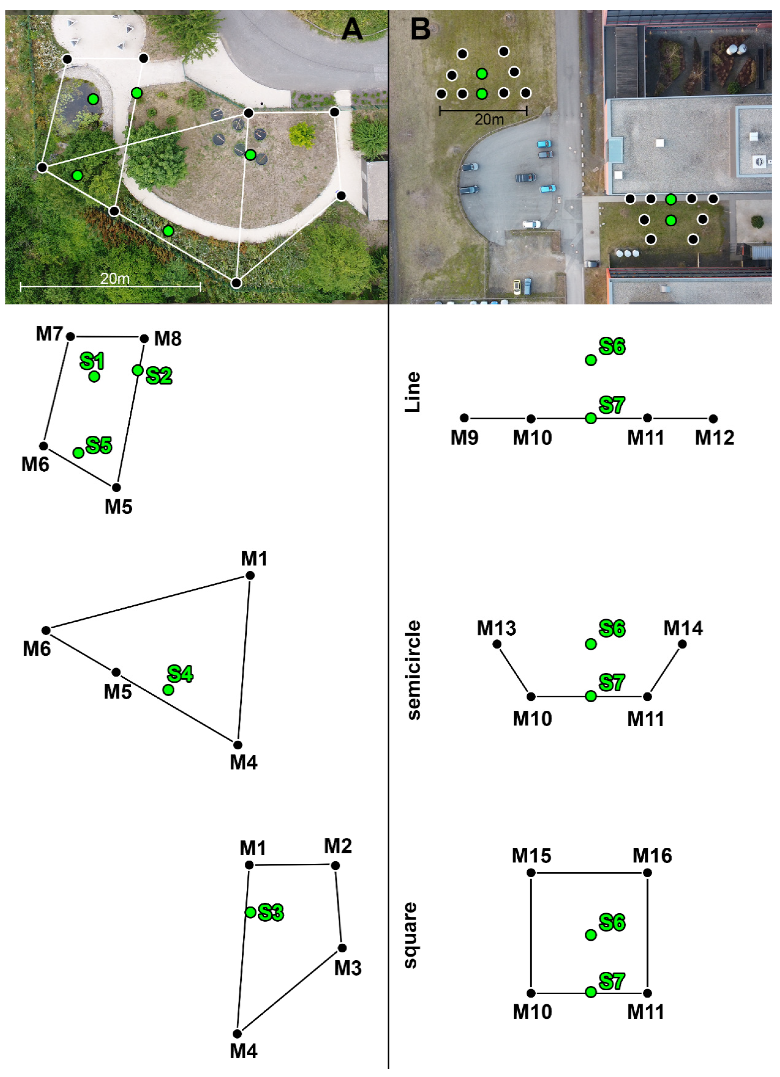
To validate the accuracy, two fixed microphone setups were set up under different conditions and the distance between the coordinates of the actual sound source and the coordinates of the center of mass of the intersections determined by the software LASER was calculated. The arrangement of the microphones for each setup is shown in Figure 1.
Recordings were made with the Zoom f8n field audio recorder (Zoom Corp., Chiyoda, Tokyo, Japan) with a sample rate of 96 kHz and eight Sennheiser ME66 microphones (Sennheiser, Wedemark-Wennebostel, Germany) covered with Rycote Windjammers (Rycote Microphone Windshields Ltd., Gloucestershire, UK). In order to determine the exact coordinates of the microphones and positions of the sound source, the Stabila LD 520 laser range finder (Stabila, Annweiler am Trifels, Germany) was used to measure the distance between the microphones and the positions of the sound sources. Data were then transferred to a digital map. The maps were created to scale using a drone (Mavic Mini, DJI, Shenzhen, Guangdong, China) in combination with a satellite map from Google maps. The area inside the microphones is 695 m2 for Setup1 and 150 m2 for Setup2. The conditions were tested with the corresponding setup as follows:
| Setup1 (environmental impact): | wind |
| dense vegetation/open space | |
| Setup2 (artificial impact): | reverb |
| microphone arrangement |
The wind speed was measured by the HT-9819 Thermo Anemometer (HTI, Dongguan, Guangdong, China) and the temperature by the EL-USB-2 data logger (Lascar electronics, Wiltshire, UK). Wind speed was always measured at the particular position where the sounds were being played. In order to determine whether the accuracy of the localization decreases significantly above a certain wind speed, the positions estimated by the software LASER were sorted according to the wind speeds prevailing at the corresponding times. Since 6 m/s was the strongest wind speed, 6 groups resulted, starting with the first group with 0–1 m/s up to the last group with 5–6 m/s. The temperature was measured by the data logger every 30 s in the shade, so that the temperature prevailing at this time could be used for each sound localization. For each position of the sound source, the same four microphones were used for localization. Theoretically, three microphones would be sufficient for a two-dimensional localization, but for more accurate results, four microphones should be used [30].
In Setup1 (environmental impact) the microphones were positioned at two different height levels due to the sloping nature of the subsoil. Microphones M1–M4 were nearly at the same height and microphones M5–M8 were nearly at the same height (Table 1 and Figure 1A).
In Setup2 (artificial impact), all microphones had the same height of 1.2 m. For each setup, a Bluetooth speaker (Ultimate Ears Megaboom 2, Logitech, Apples, Switzerland) was placed at different positions (green dots in Figure 1A,B) at which three different sounds were played. These were three vocalizations with different characteristics, a high harmonic, a low harmonic and a noisy caw (Figure 2A–C), to determine the influence of different vocalization types in sound localization. Each vocalization was played 10–20 times per run and at each position, with a constant volume between 76 and 78 dB (measured with a VOLTCRAFT SL-100 (Conrad Electronic, Hirschau, Germany) at 1 m distance). The microphone combinations used for the corresponding positions are shown in Figure 1A,B.
Setup1 (environmental impact) was set up on four different days (four runs), which differed in terms of wind speed (between 0 to 6 m/s). The sound sources S1–S4 were positioned on open spaces with few obstacles (Figure 1A). S5 was located in a treetop.
To test the accuracy of sound localization in dense vegetation playback runs with the Bluetooth speaker positioned on the ground in dense vegetation were carried out at positions S4 and S5, which will be referred to as S4ground and S5ground in the following. Since S4ground and S5ground were at ground level, creating a considerable height difference to the microphones, an error automatically occurred at these positions as the sound localization was only performed in two dimensions (see Section 2.6 “Simulations”). To localize the vocalizations played back at position S4 microphones of two different height levels (Figure 1A and Table 1) were used, so an error also occurred here due to the two-dimensional localization. At all other positions, the speaker was placed at nearly the same height as the microphones.
For Setup2 (artificial impact), the microphone positioning was tested in different arrangements with four microphones as follows: four microphones in a straight line (M9–M12), four microphones as a semicircle (M10, M11, M13, and M14) and four microphones as a square around the sound source (M10, M11, M15, and M16) (Figure 1B). The sound source (S6 and S7 in Figure 1B) was once placed directly in the middle of the area (S6) and once between the microphones M10 and M11 (S7), which leads to different localization challenges. Two application scenarios were tested, one for animals in the middle of the enclosure and one for animals at the edge of the enclosure.
The first run with Setup2 (artificial impact) was performed on open space to verify if the positioning of the microphones is important. Reverberation is a major problem when determining the TDOA, since the reflected sound event is detected by the microphone shortly after the actual sound event. This additional and time-delayed signal can lead to a significantly worse result of the cross-correlation and thus to a reduced accuracy in localization. In order to simulate a reverberant environment of a zoo enclosure, the second run was conducted between two close buildings with glass fronts. The microphones M9–M12 were placed directly at the building wall.
2.4. Frequencies
In order to evaluate whether certain frequency ranges lead to better results in dense vegetation or in a reverberant environment, four different filter settings were used. To use low frequencies and cut off high frequencies, a range between 0.2 kHz and 4 kHz was used. This filter setting is based on the lowest harmonic vocalization (Figure 2C), but still includes the most important frequency ranges and omit high frequency formants. For the middle frequency range, two slightly different filter settings were chosen (2–10 kHz and 3–10 kHz), since the most dominant formant-like structures occur in this range (compare Figure 2A–C) and a slight change in this range could already have a large impact on the determination of the TDOA. To determine whether even weakly pronounced frequencies are sufficient to determine the TDOA, a filter setting of 7–10 kHz was chosen at which none of the vocalizations used still had well pronounced frequencies. At each position of the setups used, the corresponding vocalizations were localized using all four filter settings to compare the resulting accuracies.
2.5. Field Test in the Zoo
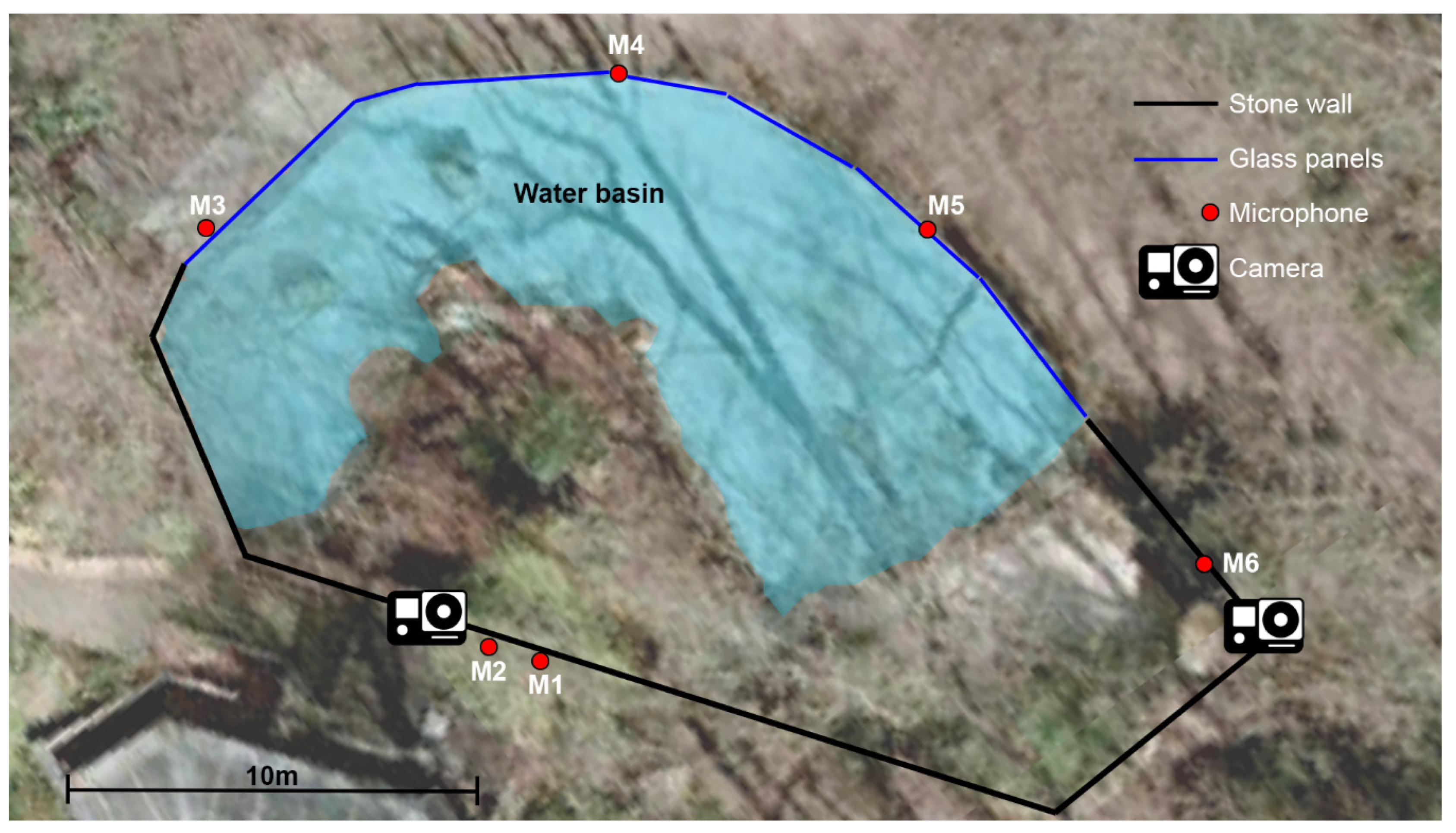
In order to test for usability of the software LASER under real conditions, a microphone setup was carried out at Dortmund Zoo in Germany at the giant otters’ enclosure. There are several reasons for selecting giant otters as a test species in zoos. Giant otters are characterized by frequent and loud calls of vocalizing individuals [32]. Furthermore, single individuals can be identified by contact calls [32] and the vocal repertoire of adult and neonate giant otters is known [33]. With regard to individual identification, studies in captive groups are much easier, on the one hand due to the small observation distance and on the other hand due to better possibilities of visual control (e.g., video recordings of the vocalizing animals). However, even under these optimal conditions, it is not always possible to clearly identify individual vocalizations [34]. The enclosure was inhabited by four adult giant otters (Pteronura brasiliensis) at the time of recording. The enclosure and the positions of the devices are shown in Figure 3. For the recordings, two connected Tascam DR-680 MkII recorders (TEAC, Tama, Tokyo, Japan) were used to which eight the t.bone EM 9900 microphones (Thomann, Burgebrach, Germany) were connected. The microphones were placed at a height of approximately 2 m to rise above the enclosure boundary. The sample rate was set to 96 kHz. The recordings took place only in the outdoor enclosure. A large part of the enclosure boundary consists of glass panes about 2 m high (Figure 3), the rest of the enclosure is bordered by stone walls of about the same height. A large water basin has been created for the otters, which takes up a large part of the outdoor area. In addition, visitors and surrounding animals created a loud background noise, while the glass walls and the water in the pool created a reverberant environment. All these factors created extremely difficult conditions for sound localization. As the giant otters were very active during the recording and constantly in motion, the sound localization could also be validated for moving sound sources. During audio recordings, the otters’ positions and behavior patterns were recorded with two GoPro Hero4 Silver cameras (GoPro Inc., San Mateo, CA, USA). By combining these two methods, the real position of the otter could be compared to the position estimated by the software LASER.
For estimating the accuracy under real conditions, i.e., without knowing the actual position of the vocalizing animal, we used the area (A) of the smaller ellipse, containing 50% of the intersects (see Section 2.2). As an error value for the evaluation, the resulting radius (r) was determined using the formula:
r = sqrt(A/pi).
Video recordings were used to track whether one or more otters were within the area of the smaller ellipse. If only one animal was within this area, it was counted as an “individual detected”; if multiple otters were within this area, it was counted as a “location detected”. If none of the animals were within the small ellipse, the localization was counted as “not detected”. The recording duration was 2 h and 52 vocalizations were evaluated. Two vocalizations were discarded because the vocalizing animal was not within the outdoor enclosure. For each vocalization, the best microphone combination and frequency filter settings were selected based on the best respectively lowest resulting value of quality, and the results of the localization performed with these settings were used.
2.6. Simulations
Two problems can arise when setting up microphone arrays in zoos: first, errors can occur when measuring the exact coordinates of the microphones, and second, it is often not possible to install all microphones at the same height, which can lead to inaccuracies in a two-dimensional sound localization. Since deviations from the original position due to these two factors can be determined mathematically more accurately than by field tests, two simulations were programmed to calculate the corresponding deviations. To simulate the accuracy deviation due to measurement errors, a measurement inaccuracy at each microphone in Setup1 (environmental impact) of 0.05 m was assumed. Simulations were performed both with a measurement error toward and away from the sound source. The simulations resulted in an average accuracy deviation of 0.056 m ± 0.018 m.
To simulate the accuracy deviation due to height differences between sound source and receiver in two-dimensional localizations, the height difference between the positions of the Bluetooth speaker at ground level and the height of the microphones was measured (Table S1A). The difference between the position estimated by the simulation and the real position is taken as the accuracy deviation (Table S1B).
For both simulations a temperature of 20 °C was assumed.
2.7. Statistical Analysis
Our study uses the deviation between the position determined by the software LASER and the actual position of the sound source in meters to verify the accuracy of the sound localization. At all sound source positions specified in Setup1 and 2, the three vocalizations were each played 10 to 15 times per experimental day. This results in between 30 and 45 recordings per test day for each position. To avoid pseudoreplication and to ensure that only representative values were used for statistical evaluation, only the one corresponding to the median for each vocalization and position was selected from the 10 to 15 accuracy values. For the evaluation of the microphone arrays, the filter setting with the best value for quality was selected.
Since under real conditions in the zoo the position of the vocalizing animal is unknown, the software LASER calculates a value for the quality of the sound localization, which serves to estimate the accuracy. Similar to Wilson et al. [18], a mixed effects model is used to show that the value for “quality” can be used to estimate the reliability of the estimated position of the vocalizing animal, when the actual position is unknown. The value for quality was taken as a fixed effect, distance in meters from the true position of the Bluetooth speaker (accuracy) as a dependent variable. Since the same vocalizations were played at the same position, “position” was added as a random effect to resolve the non-independence. Furthermore, the three vocalizations, the days of testing and the tested frequencies were also added as a random effect, so that the following formula was used:
Accuracy ~ quality + (1|position) + (1|vocalization) + (1|date) + (1|frequency).
Since residuals were not normally distributed, accuracy, and quality were log10-transformed. All assumptions were then satisfied.
To test whether various factors significantly improved or degraded the accuracy of the sound localization, the Friedman test was used for dependent samples and the Kruskal–Wallis test for independent samples, since all samples were not normally distributed. A Turkey post-hoc test was performed for the pairwise comparison. All tests were performed using the Statistics and Machine Learning Toolbox in MATLAB. A value of p < 0.05 was considered significant.
3. Results
The software LASER estimated the position of the sound source under the given conditions in Setup1 (environmental impact) with a median accuracy of 0.234 m and a median quality of 4.074 (N = 72). The simulation to determine the deviations due to measurement errors showed an average deviation of 0.056 m ± 0.018 m for Setup1 (environmental impact). The linear mixed model applied to the data from Setup1 (environmental impact) verifies that the value for quality estimates the accuracy of sound localization in a highly significant way (F(1.214) = 160.91, N = 216, p < 0.001). This makes it possible to determine the reliability of sound localization even under real conditions when the position of the desired vocalizing animal is not known. Higher values for the quality indicate a greater deviation from the actual position. In addition, the model estimates an intercept at 0.0596 m, which is very close to the error determined by the simulation (0.056 m).
3.1. Wind
A Kruskal–Wallis test showed no significant differences (Chi2 = 6.41, N = 360, p = 0.2683) between the six different wind speed groups (0–1 m/s; 1–2 m/s; 2–3 m/s; 3–4 m/s; 4–5 m/s; and 5–6 m/s). Therefore, it can be concluded that wind up to a speed of 6 m/s has no considerable influence on the accuracy in a setup of this size.
3.2. Dense Vegetation and Open Space
The median accuracy for the positions in open space (S1–S4) is 0.213 m. In comparison, the median accuracy for the two positions in dense vegetation S4ground and S5ground is 0.45 m. Although the deviation of the localization in dense vegetation is more than twice as large as in open space, a deviation of 0.45 m is still in a suitable range compared to the size of the area covered inside the microphones (695 m2), especially if the error due to the difference in height is taken into account. Since only two-dimensional localization was used in this study, height differences between the microphones and the sound source play a role in the accuracy of the estimated position. A simulation was used to determine the deviation when the sound source was positioned on ground level at each position instead of the height of the microphones (Table S1B). This is especially important for the positions S4ground and S5ground, which were used to verify the accuracy in dense vegetation, because they were not positioned at microphone level, but on the ground. The simulation calculated a deviation from the actual position to be expected due to the height difference of 0.148 m for S4ground and 0.292 m for S5ground. Subtracting the mean value of the simulated deviation (0.22 m) from the determined accuracy (0.45 m) yields a corrected deviation of 0.23 m.
Different frequency ranges were used for localization at each position to evaluate which frequency range leads to the best results in dense vegetation. Therefore, the accuracies at positions S4ground and S5ground determined by means of the corresponding frequency ranges were tested against each other using a Friedman test. Since the test gave a highly significant result (Chi2 = 17.6, N = 18, p < 0.001), a subsequent post-hoc test was performed, which showed a highly significant difference between the frequency ranges 0.2–4 kHz and 3–10 kHz (p = 0.0017) and between 0.2–4 kHz and 7–10 kHz (p = 0.0017). The results are shown in Figure 4C. The best accuracies in dense vegetation were achieved when filtering with the frequency range 0.2–4 kHz. Therefore, we suggest to use low frequencies in dense environments for sound localization. In addition, a Friedman test was applied in the same way to positions on open space to investigate which frequency range is best suited for localization in such an environment. Again, there seem to be differences in the frequency ranges used, as the test led to a significant result (Chi2 = 12.6533, N = 54, p = 0.0054). A post-hoc test performed afterwards showed significant differences for the frequency ranges 2–10 kHz and 0.2–4 kHz (p = 0.012) and for 2–10 kHz and 7–10 kHz (p = 0.0239). The results are shown in Figure 4B. In open space, localization with higher frequencies in the range of 2–10 kHz seems to be advantageous, although the fundamental frequency and most of the dominant frequencies are omitted. Since position S5 was in a treetop, but at the level of microphones M1–M4, it is difficult to compare with the other positions. At this position a median accuracy of 0.25 m was achieved. For 44.44% of the sound localizations at this position, a filter setting of 0.2–4 kHz provided the best value for the quality, for 33.33% a filter setting of 2–10 kHz provided the best value for the quality and for 22.22% a filter setting of 3–10 kHz provided the best value for the quality.
3.3. Microphone Arrangement
Three different microphone arrangements were tested using Setup2 (artificial impact). A straight line (M9–M12), a square arrangement enclosing the sound source (M10, M11, M15, and M16) and a semi-circular arrangement (M10, M11, M13, and M14; Figure 1B). The accuracies of the respective arrangements were compared with each other using a Friedman test. The test suggests a highly significant difference (Chi2 = 30.9556, N = 90, p < 0.001) between the arrangements, after which a post-hoc test was performed. This test shows highly significant differences between the square arrangement (median = 0.063 m) and the other two arrangements (for each p < 0.001; Figure 4D). Nevertheless, the accuracy for the other two arrangements is still good (median(line) = 0.195 m; median(semicircle) = 0.208 m).
3.4. Reverb
Setup2 (artificial impact) was used to test whether filtering in certain frequency ranges or the arrangement of the microphones could reduce a deterioration in accuracy caused by reverberation. For comparing the three frequency ranges (0.2–4 kHz, 2–10 kHz, and 7–10 kHz) the microphones M10, M11, M15, and M16 were used (square in Figure 1B). A Friedman test showed no significant difference (Chi2 = 5.8333, N = 60, p = 0.0541). When testing with different microphone arrangements (filter settings at 2–10 kHz), however, a highly significant difference was found (Friedman test: Chi2 = 135.6047, N = 60, p < 0.001). The post-hoc test revealed that if the microphones M9–M12 were placed in a straight line directly at the reverberating wall, they showed a highly significant deviation compared to all other arrangements (for each p < 0.001) (Figure 4E). Considering that the filter settings have not been adapted to the sound event (for example, in the case of background noise such as birdsongs) the microphone arrangements “square” and “semicircle” show only small deviations from the actual position.
3.5. Vocalization Types
The results obtained for each vocalization showed no significant differences in localization accuracy (Kruskal–Wallis: Chi2 = 0.05, N = 24, p = 0.9744).
3.6. Field Test in the Zoo
Results show that, the software LASER was able to determine the position of the vocalizations in 96% of cases (N = 50; Figure 5). Furthermore, in 78% of the cases, the position of single individuals could be clearly identified, although the animals were mostly in close proximity (Figure 5 and Figure 6).
Despite the fact that in 14% of cases the position was accurately estimated and the ellipse spanned a very narrow area (median r = 0.287 m; A = 0.259 m2), the individual could not be identified merely because two individuals within the estimated area were extremely close to each other. Only in 4% of the cases (two vocalizations) the position of the vocalizing animal was not correctly identified. In both cases a sufficiently good quality could not be achieved (best results: 11.37 and 15.6). The overall median size of the determined area around the estimated positions is 0.58 m2 (r = 0.43 m), which is considerably smaller compared to the body size of a giant otter.
4. Discussion
The software LASER presented here is able to estimate the localization of vocalizing animals very accurately, allowing even the discrimination of single individuals in a small area. The validation of the localization for its accuracy revealed a median deviation from the actual position of 0.234 m within an area of 695 m2. This high accuracy is based on the fact that the TDOA is determined via the spectrogram as well as the oscillogram. If only spectrograms had been used to determine TDOA, the accuracy would have been limited to approximately 0.73 m (at 20 °C), which is low indeed, since the time resolution of the spectrograms in this study is only 2.135 ms due to a 90% overlap of the windows and a sample rate of 96 kHz. Since many software approaches are used to estimate the position of vocalizing animals in the field and thus in large areas, usually only the spectrogram is used to determine the TDOA [18,23,24]. However, this limits their accuracy due to the low time resolution and makes them less suitable for use in zoos. Sound localization is also used for livestock, for example, to monitor the health of the animals in the barn [25,26]. Here, the accuracy must be significantly better due to the close proximity of the animals, so that in these cases the TDOA is usually determined by cross-correlation of the oscillogram [25,26]. It is accepted that a cross correlation by means of the oscillogram is much more susceptible to a bad SNR, because the barn is well protected from external noise. Furthermore, in this case only one animal species or often even only one specific vocalization, which indicates a possible disease, is of interest, which means that a frequency filter only needs a specific setting. However, a software approach for zoos must not only be robust against noise, but also as accurate as possible and additionally flexible in the application of the filter settings, as the software should cover as many different vocalizations and enclosure characteristics as possible. All this is offered by the software LASER.
Since the position of the sound source is not known under real conditions, it is essential that the estimated position can be reliably assessed. In this context, the determined value for the quality of localization represents a suitable measurement parameter. Using a linear mixed model, it could be shown that this value can predict the accuracy of the localization in a highly significant way. Thus it is not only possible to reject unreliable results, but also to repeat the localization with different settings to improve the accuracy.
4.1. Influence of Various Conditions and Filter Settings on the Accuracy of Sound Localization
The accuracy of the software LASER has been tested under various conditions, including wind, dense vegetation, and a reverberant environment. At wind speeds up to 6 m/s, no influence on the localization could be detected.
In dense vegetation it is more difficult to obtain an accurate result due to the effects of surrounding obstacles, such as leaves, branches, or trunks [28]. Despite the additional large height difference at the corresponding positions with dense vegetation, an accurate median result was achieved (see Section 3.2). The filter settings chosen are important for accurate determination. Therefore, for position determination in dense vegetation, if possible, the TDOA should be determined using low frequencies, since dense vegetation has a greater effect on higher frequencies [27,28]. In general, the filter settings should be evaluated individually for each localization. Even if a vocalization is emitted in dense vegetation, noise in the low frequency range could lead to a worse result if a low band pass filter is used. In open spaces, environmental noise is more likely to occur below 2 kHz, so SNR is better above 2 kHz [35]. Furthermore, low frequencies can travel longer distances than higher frequencies [27], which means that low frequencies from disturbing noises are more likely to reach the microphones than high frequencies. Our study demonstrates that a localization with only formant-like structures and without the dominant frequency in lower ranges leads in some cases to much more accurate results compared to a sound localization including the low frequencies. In addition, a targeted setting of the frequency filter should be used to minimize the influence of noise from visitors or surrounding animals in the zoo and to achieve good results.
4.2. Influence of Microphone Arrangement on the Accuracy of Sound Localization
In general, it is better to localize in three dimensions and take the height into account. Unevenness in the enclosure makes it difficult to position the microphones accurately with respect to the height difference, so all localizations in this study were performed in two dimensions. However, the influence of the height differences on the accuracy (Table S1B) is in an acceptable range in relation to the size of the test area. It could also be shown that a reasonable positioning of the microphones can improve the accuracy of the localization. If the microphones are placed around the area, one is more flexible in selecting the right microphones. With the surrounding arrangement, the user has the possibility to select the microphones for localization specifically. Individual microphones that lead to poorer results are reliably detected and excluded on the basis of the quality value.
Reverberation is a major problem in zoos when conducting sound localizations and dealing with it is an important aspect. Especially in zoos, however, glass panels are often used as boundaries to provide visitors with the best possible view into the enclosures. Since glass has a low absorption coefficient, it reflects sound strongly [36]. The air-water interface is also reflective to sounds and should be taken into account as a reverberant surface [35]. The positioning of the microphones seems to play a crucial role in solving this problem. If microphones are selected whose distance from the sound source or the reverberating object differs greatly, it becomes much more difficult to determine the TDOA using cross-correlation. This is due to the considerably different arrival time of the reverb event at the microphones. Presumably this is the reason why the results of the line arrangement in Setup2 (artificial impact) are significantly worse than all other microphone arrangements in the reverberant environment. Nevertheless, considering that the filter settings have not been adapted to the sound event (for example, in the case of background noise such as birdsongs) the microphone arrangements “square” and “semicircle” show similarly accurate results as a sound localization in a reverberation-free environment.
4.3. Applying the Software LASER to Zoo Conditions and Limitations
In this study, video recordings were used for evaluation to verify sound localization and individual recognition via the software LASER. Despite the difficult and reverberant environment, the results with the giant otters in Dortmund Zoo show a high reliability (correct localization in 96% of the cases). The results show that a microphone array consisting of several microphones is favorable because the appropriate microphones can be selected via the software LASER. The selection of the most suitable microphones can be estimated by the best resulting value for quality, as well as by the usefulness of the spectrogram respectively its SNR. When microphones with a significant distance difference from the vocalizing animal were combined, their TDOA negatively affected the quality due to the reverberant environment, and thus the accuracy of localization. Furthermore, a flexible application of the frequency filters is crucial. Since some of the otter calls had formant-like structures, which were still clearly recognizable up to 16 kHz (compare [32,33]), it was possible to cut off interfering noise in lower frequencies to improve the results. However, not only the environment made the conditions for sound localization more difficult, but also the fact that the otters were constantly on the move, as a group, close together. Although animals were moving close together, 78% of the vocalizations could be assigned to the corresponding individual. This high hit rate can be achieved because the determined area for the vocalizing animal is very small, 0.58 m2 (r = 0.43 m), and well below the size of a single giant otter. This finding may open new possibilities to characterize the communication between individuals of a group in more detail.
Nevertheless, there are certainly situations in which sound localization reaches its limits. An important prerequisite is that the vocalizations should be loud enough to achieve good results. The calls of giant otters are very loud and therefore well suited, whereas animals that vocalize very softly are probably rather unsuitable due to a worse SNR [18]. The loudness of animal calls can also become a problem in very large enclosures. When microphones and sound source are far apart, the sound event will arrive at the microphones attenuated due to the long distance and possible obstacles between the vocalizing animal and the microphones. This has negative consequences for SNR and, thus, for sound localization [29,37]. Since a vocalization should be well captured by at least 4 microphones for a two-dimensional localization [30], a correspondingly higher number of microphones is therefore advisable for large enclosures in order to capture all areas within the enclosure. The advantage of the software LASER is that the most suitable microphones can be selected in order to achieve the best possible results even in large enclosures. In addition, not all enclosures allow an advantageous positioning of the microphones, which makes an accurate localization more difficult. In the future, it should also be tested whether sound localization can work well in halls and domes. The increased background noise and the highly reverberant environment pose a great challenge.
4.4. Bioacoustics and Sound Localization as Contribution to Animal Welfare in Zoos
Studies of vocal behavior allow conclusions to be drawn about an animal’s physiological state, which may reflect both physiological and psychological aspects of well-being [38,39,40,41].
Social bonds between individuals, for example, have a positive influence on health status, animal welfare, and lifelong reproductive performance [42]. By using the software LASER presented here, the analysis can contribute additional parameters for both negative and positive contexts. For example, position determination can be used to determine the possible influence of enclosure structures (without recording image data). In most studies animal-attached technology is preferred for monitoring individuals, but this is not feasible for all species, especially zoo animals. Our results show that the software LASER used is able to reliably identify single individuals via the high spatial resolution. In combination with individually distinguishable calls, this also offers the possibility to characterize single individuals in more detail without visual inspection. This is especially important in enclosures or situations where the animals are difficult to observe visually because the enclosure is densely vegetated or the animals are nocturnal. Tracking the position (and behavior) of an animal based on its vocalizations is a promising alternative to visual observation here. Since automated recognition of selected vocalizations via deep learning can now be used effectively and is being used more and more frequently [43], the isolation of desired vocalizations from long-term recordings would be possible considerably faster than a human evaluation in the future. Subsequently these vocalization units can be used to estimate the position of the sound-emitting animal in the enclosure by means of sound localization. Once calls of interest (positive and/or negative) are identified, they can be monitored periodically to establish baseline rates for individuals. In summary, acoustic activity may be an important indicator of animal welfare and could be used to assess the effects of animal transfers, introductions, group behavior, and environmental changes.
5. Conclusions
In summary, the software LASER provides very accurate results even under difficult recording conditions, for example in zoos. It even allows reliable detection of vocalizing individuals within a group. In combination with an automated analysis of the bioacoustics data, long-term monitoring would be possible in the future, identifying calls of interest (positive and/or negative) and collecting information on behavioral aspects, social structures, and animal welfare. In case of an interest in the software LASER, it is accessible for scientific purposes upon reasonable request by the corresponding author.
Supplementary Materials
The following are available online at https://0-www-mdpi-com.brum.beds.ac.uk/article/10.3390/jzbg2020011/s1, Figure S1: LASER user interface and result example, Table S1: Height difference between microphone and the corresponding sound source on the ground and the resulting accuracy deviations.
Author Contributions
Conceptualization, S.S. and P.W.D.; methodology, S.S. and P.W.D.; software, S.S.; validation, S.S.; formal analysis, S.S.; investigation, S.S.; data curation, S.S.; writing—original draft preparation, S.S.; writing—review and editing, P.W.D.; visualization, S.S. and P.W.D.; supervision, P.W.D.; project administration, P.W.D.; funding acquisition, P.W.D. All authors have read and agreed to the published version of the manuscript.
Funding
This research was financially supported by Opel-Zoo foundation professorship in zoo biology from the “von Opel Hessische Zoostiftung”.
Institutional Review Board Statement
The study was conducted according to the guidelines of EEP Coordinator Tim Schikora.
Informed Consent Statement
Not applicable.
Acknowledgments
The authors are very grateful to Opel-Zoo Kronberg and Zoo Dortmund for their continued support and for their valuable feedback. We would also like to thank Niko Schneider for his support in programming the software LASER.
Conflicts of Interest
The authors declare no conflict of interest. The funders had no role in the design of the study; in the collection, analyses, or interpretation of data; in the writing of the manuscript, or in the decision to publish the results.
References
- Volodina, E.; Volodin, I.A. Bioacoustics in zoos: A review of applications and perspectives. Int. Zoo News 1999, 46, 208–213. [Google Scholar]
- Geissmann, T. Inheritance of song parameters in the gibbon song, analysed in 2 hybrid gibbons (Hylobates pileatus× H. lar). Folia Primatol. 1984, 42, 216–235. [Google Scholar] [CrossRef]
- Long, A.M.; Moore, N.P.; Hayden, T.J. Vocalizations in red deer (Cervus elaphus), sika deer (Cervus nippon), and red× sika hybrids. J. Zool. 1998, 244, 123–134. [Google Scholar] [CrossRef]
- Wyman, M.T.; Locatelli, Y.; Charlton, B.D.; Reby, D. Female sexual preferences toward conspecific and hybrid male mating calls in two species of polygynous deer, cervus elaphus and c. nippon. Evol. Biol. 2016, 43, 227–241. [Google Scholar] [CrossRef] [PubMed] [Green Version]
- Semple, S.; McComb, K. Perception of female reproductive state from vocal cues in a mammal species. Proc. Biol. Sci. 2000, 267, 707–712. [Google Scholar] [CrossRef] [Green Version]
- Buesching, C.; Heistermann, M.; Hodges, J.; Zimmermann, E. Multimodal oestrus advertisement in a small nocturnal prosimian, Microcebus murinus. Folia Primatol. 1998, 69, 295–308. [Google Scholar] [CrossRef]
- Lindburg, D.G. Proceptive calling by female lion-tailed macaques. Zoo Biol. 1990, 9, 437–446. [Google Scholar] [CrossRef]
- Moos-Heilen, R.; Sossinka, R. The influence of oestrus on the vocalization of female gelada baboons (Theropithecus gelada). Ethology 1990, 84, 35–46. [Google Scholar] [CrossRef]
- Volodin, I.; Kaiser, M.; Matrosova, V.; Volodina, E.; Klenova, A.; Filatova, O.; Kholodova, M. The technique of noninvasive distant sexing for four monomorphic dendrocygna whistling duck species by their loud whistles. Bioacoustics 2009, 18, 277–290. [Google Scholar] [CrossRef]
- Carlson, G.; Trost, C.H. Sex determination of the whooping crane by analysis of vocalizations. Condor 1992, 94, 532–536. [Google Scholar] [CrossRef]
- Volodin, I.A.; Volodina, E.V.; Klenova, A.V.; Matrosova, V.A. Gender identification using acoustic analysis in birds without external sexual dimorphism. Avian Res. 2015, 6, 1–17. [Google Scholar] [CrossRef] [Green Version]
- Laporte, M.N.; Zuberbühler, K. Vocal greeting behaviour in wild chimpanzee females. Anim. Behav. 2010, 80, 467–473. [Google Scholar] [CrossRef] [Green Version]
- Aich, H.; Moos-Heilen, R.; Zimmermann, E. Vocalizations of adult gelada baboons (Theropithecus gelada): Acoustic structure and behavioural context. Folia Primatol. 1990, 55, 109–132. [Google Scholar] [CrossRef] [PubMed]
- Fischer, J.; Wegdell, F.; Trede, F.; Dal Pesco, F.; Hammerschmidt, K. Vocal convergence in a multi-level primate society: Insights into the evolution of vocal learning. Proc. R. Soc. B 2020, 287, 20202531. [Google Scholar] [CrossRef] [PubMed]
- Briefer, E.F. Vocal expression of emotions in mammals: Mechanisms of production and evidence. J. Zool. 2012, 288, 1–20. [Google Scholar] [CrossRef] [Green Version]
- Jürgens, U. Vocalization as an emotional indicator. A neuroethological study in the squirrel monkey. Behaviour 1979, 69, 88–117. [Google Scholar] [CrossRef]
- Schön, P.C.; Puppe, B.; Manteuffel, G. Automated recording of stress vocalization as a tool to document impaired welfare in pigs. Anim. Welf. 2004, 13, 105–110. [Google Scholar]
- Wilson, D.R.; Battiston, M.; Brzustowski, J.; Mennill, D.J. Sound Finder: A new software approach for localizing animals recorded with a microphone array. Bioacoustics 2014, 23, 99–112. [Google Scholar] [CrossRef] [Green Version]
- Wijers, M.; Loveridge, A.; Macdonald, D.W.; Markham, A. CARACAL: A versatile passive acoustic monitoring tool for wildlife research and conservation. Bioacoustics 2021, 30, 41–57. [Google Scholar] [CrossRef]
- Collier, T.C.; Kirschel, A.N.G.; Taylor, C.E. Acoustic localization of antbirds in a Mexican rainforest using a wireless sensor network. J. Acoust. Soc. Am. 2010, 128, 182–189. [Google Scholar] [CrossRef] [Green Version]
- Mennill, D.J.; Burt, J.M.; Fristrup, K.M.; Vehrencamp, S.L. Accuracy of an acoustic location system for monitoring the position of duetting songbirds in tropical forest. J. Acoust. Soc. Am. 2006, 119, 2832–2839. [Google Scholar] [CrossRef] [Green Version]
- Spiesberger, J.L.; Fristrup, K.M. Passive localization of calling animals and sensing of their acoustic environment using acoustic tomography. Am. Nat. 1990, 135, 107–153. [Google Scholar] [CrossRef]
- Kershenbaum, A.; Owens, J.L.; Waller, S. Tracking cryptic animals using acoustic multilateration: A system for long-range wolf detection. J. Acoust. Soc. Am. 2019, 145, 1619. [Google Scholar] [CrossRef] [PubMed] [Green Version]
- Frommolt, K.-H.; Tauchert, K.-H. Applying bioacoustic methods for long-term monitoring of a nocturnal wetland bird. Ecol. Inform. 2014, 21, 4–12. [Google Scholar] [CrossRef]
- Exadaktylos, V.; Silva, M.; Ferrari, S.; Guarino, M.; Taylor, C.J.; Aerts, J.-M.; Berckmans, D. Time-series analysis for online recognition and localization of sick pig (Sus scrofa) cough sounds. J. Acoust. Soc. Am. 2008, 124, 3803–3809. [Google Scholar] [CrossRef]
- Silva, M.; Ferrari, S.; Costa, A.; Aerts, J.-M.; Guarino, M.; Berckmans, D. Cough localization for the detection of respiratory diseases in pig houses. Comput. Electron. Agric. 2008, 64, 286–292. [Google Scholar] [CrossRef]
- Marten, K.; Marler, P. Sound transmission and its significance for animal vocalization. Behav. Ecol. Sociobiol. 1977, 2, 271–290. [Google Scholar] [CrossRef]
- Richards, D.G.; Wiley, R.H. Reverberations and amplitude fluctuations in the propagation of sound in a forest: Implications for animal communication. Am. Nat. 1980, 115, 381–399. [Google Scholar] [CrossRef]
- Rhinehart, T.A.; Chronister, L.M.; Devlin, T.; Kitzes, J. Acoustic localization of terrestrial wildlife: Current practices and future opportunities. Ecol. Evol. 2020, 10, 6794–6818. [Google Scholar] [CrossRef]
- Spiesberger, J.L. Hyperbolic location errors due to insufficient numbers of receivers. J. Acoust. Soc. Am. 2001, 109, 3076–3079. [Google Scholar] [CrossRef]
- Wölfel, M.; McDonough, J. Distant Speech Recognition; John Wiley & Sons, Ltd.: West Sussex, UK, 2009; ISBN 9780470714089. [Google Scholar]
- Mumm, C.A.; Urrutia, M.C.; Knörnschild, M. Vocal individuality in cohesion calls of giant otters, Pteronura brasiliensis. Anim. Behav. 2014, 88, 243–252. [Google Scholar] [CrossRef]
- Mumm, C.A.S.; Knörnschild, M. The vocal repertoire of adult and neonate giant otters (Pteronura brasiliensis). PLoS ONE 2014, 9, e112562. [Google Scholar] [CrossRef]
- Mumm, C.A.S.; Knörnschild, M. Territorial choruses of giant otter groups (Pteronura brasiliensis) encode information on group identity. PLoS ONE 2017, 12, e0185733. [Google Scholar] [CrossRef] [PubMed] [Green Version]
- Forrest, T.G. From sender to receiver: Propagation and environmental effects on acoustic signals. Am. Zool. 1994, 34, 644–654. [Google Scholar] [CrossRef] [Green Version]
- Rossing, T.D.; Moore, F.R.; Wheeler, P. The Science of Sound, 3rd ed.; Addison Wesley: San Francisco, CA, USA, 2002; ISBN 0-8053-8565-7. [Google Scholar]
- Papin, M.; Pichenot, J.; Guérold, F.; Germain, E. Acoustic localization at large scales: A promising method for grey wolf monitoring. Front. Zool. 2018, 15, 11. [Google Scholar] [CrossRef]
- Weary, D.M.; Ross, S.; Fraser, D. Vocalizations by isolated piglets: A reliable indicator of piglet need directed towards the sow. Appl. Anim. Behav. Sci. 1997, 53, 249–257. [Google Scholar] [CrossRef] [Green Version]
- Watts, J.M.; Stookey, J.M. Vocal behaviour in cattle: The animal’s commentary on its biological processes and welfare. Appl. Anim. Behav. Sci. 2000, 67, 15–33. [Google Scholar] [CrossRef]
- Manteuffel, G.; Puppe, B.; Schön, P.C. Vocalization of farm animals as a measure of welfare. Appl. Anim. Behav. Sci. 2004, 88, 163–182. [Google Scholar] [CrossRef]
- Boissy, A.; Manteuffel, G.; Jensen, M.B.; Moe, R.O.; Spruijt, B.; Keeling, L.J.; Winckler, C.; Forkman, B.; Dimitrov, I.; Langbein, J.; et al. Assessment of positive emotions in animals to improve their welfare. Physiol. Behav. 2007, 92, 375–397. [Google Scholar] [CrossRef]
- Rose, P.E.; Croft, D.P. The potential of social network analysis as a tool for the management of zoo animals. Anim. Welf. 2015, 24, 123–138. [Google Scholar] [CrossRef] [Green Version]
- Christin, S.; Hervet, É.; Lecomte, N. Applications for deep learning in ecology. Methods Ecol. Evol. 2019, 10, 1632–1644. [Google Scholar] [CrossRef]
Figure 1.
Microphone arrangement for Setup1 (environmental impact) (A) and Setup2 (artificial impact) (B). The black dots indicate the positions of the microphones M1–M16. The green dots indicate the positions where the Bluetooth speaker was set up and the test vocalizations (Figure 2) were played (S1–S7). (A) The microphones by means of which the corresponding position of the Bluetooth speaker is estimated are shown below the aerial image (S1/S2/S5 = M5–M8; S3 = M1–M4; S4 = M1, M4–M6). (B) The microphones used for the three different microphone arrangements (square, semicircle, line) are shown below the aerial image (square = M10, M11, M15, M16; semicircle = M10, M11, M13, M14; line = M9–M12).

Figure 2.
Spectrogram (top) and corresponding spectrum (bottom) of the vocalizations played in both setups. The vocalizations differed in various features, such as duration, fundamental frequency, and if they are rather harmonic or noisy. The x-axis labeling of the spectra (bottom) is based on the filter settings used (explained later); (A) 1.5 s long harmonic vocalization with a fundamental frequency of up to F0 = 0.68 kHz; (B) 0.5 s long rather noisy vocalization (the determination of the fundamental frequency was not conducted); (C) 2.5 s long harmonic vocalization with a fundamental frequency of up to F0 = 0.2 kHz.

Figure 3.
Design of the giant otter enclosure with positions of microphones and cameras. The satellite view from Google Earth was used for the map (Image © 2021 AeroWest).
Figure 3.
Design of the giant otter enclosure with positions of microphones and cameras. The satellite view from Google Earth was used for the map (Image © 2021 AeroWest).

Figure 4.
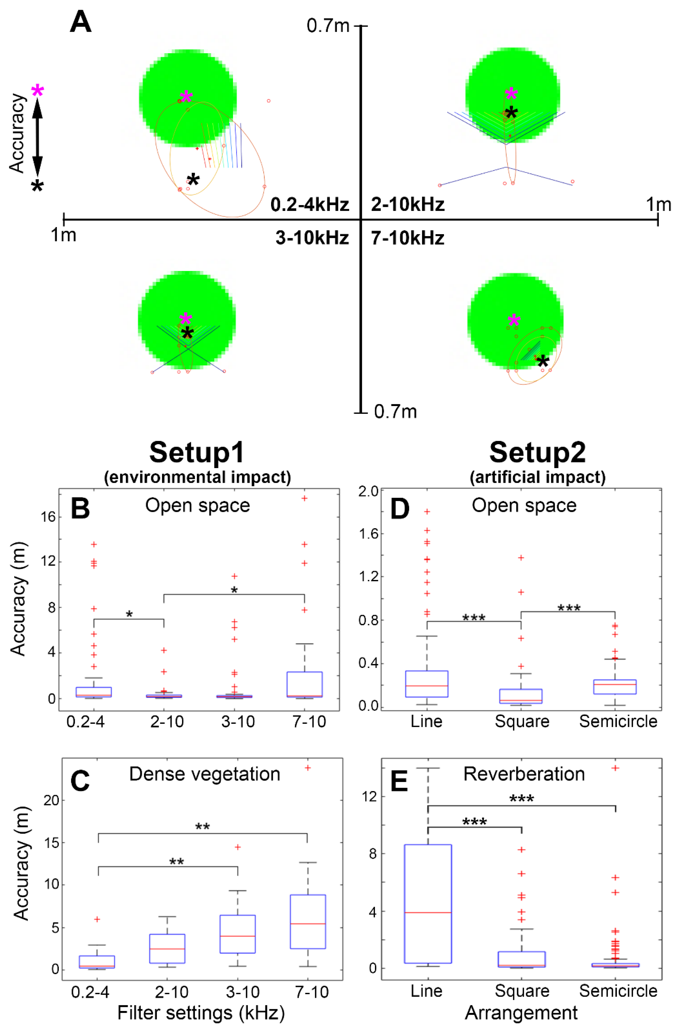
(A) Exemplary result of a sound localization. The distance between the actual position of the sound source (pink asterisk) and the position estimated via the software Localize Animal Sound Events Reliably (LASER) (black asterisk) is used to determine the accuracy. In this example, the accuracy for sound localization using a filter setting of 0.2–4 kHz is 0.284 m, the accuracy using a filter setting of 2–10 kHz is 0.069 m, the accuracy using a filter setting of 3–10 kHz is 0.049 m, and the accuracy using a filter setting of 7–10 kHz is 0.177 m. (B–E) Statistical results presented as boxplots. (B) Comparison of the influence of the used frequency range on the accuracy of sound localization in open space. (C) Comparison of the influence of the used frequency range on the accuracy of sound localization in dense vegetation. (D) Comparison of the influence of the arrangement of the microphones on the accuracy of sound localization in open space. Low-cut filter was set to 2–10 kHz. (E) Comparison of the influence of the arrangement of the microphones on the accuracy of sound localization in a reverberant environment. Low-cut filter was set to 2–10 kHz. Only significant differences are shown: (*) p ≤ 0.05; (**) p ≤ 0.01; (***) p ≤ 0.001.
Figure 4.
(A) Exemplary result of a sound localization. The distance between the actual position of the sound source (pink asterisk) and the position estimated via the software Localize Animal Sound Events Reliably (LASER) (black asterisk) is used to determine the accuracy. In this example, the accuracy for sound localization using a filter setting of 0.2–4 kHz is 0.284 m, the accuracy using a filter setting of 2–10 kHz is 0.069 m, the accuracy using a filter setting of 3–10 kHz is 0.049 m, and the accuracy using a filter setting of 7–10 kHz is 0.177 m. (B–E) Statistical results presented as boxplots. (B) Comparison of the influence of the used frequency range on the accuracy of sound localization in open space. (C) Comparison of the influence of the used frequency range on the accuracy of sound localization in dense vegetation. (D) Comparison of the influence of the arrangement of the microphones on the accuracy of sound localization in open space. Low-cut filter was set to 2–10 kHz. (E) Comparison of the influence of the arrangement of the microphones on the accuracy of sound localization in a reverberant environment. Low-cut filter was set to 2–10 kHz. Only significant differences are shown: (*) p ≤ 0.05; (**) p ≤ 0.01; (***) p ≤ 0.001.

Figure 5.
Success of sound localization for the giant otter enclosure in percent. In 96% of the cases, the software LASER was able to correctly estimate the position of the vocalization (black upper bar). Only in 4% of the cases the position could not be recognized correctly (white upper bar). The 96% are divided into 78% in which the individual emitting the sound could be detected (lower thick-striped bar), 14% in which the software LASER was able to estimate the position of the vocalizing animal very precisely and with a small probability range (ellipse spanning 50% of the intersections); however, two animals were very close to each other within this probability range (lower thin-striped bar) and 4% in which the probability range was large enough to include several individuals.

Figure 6.
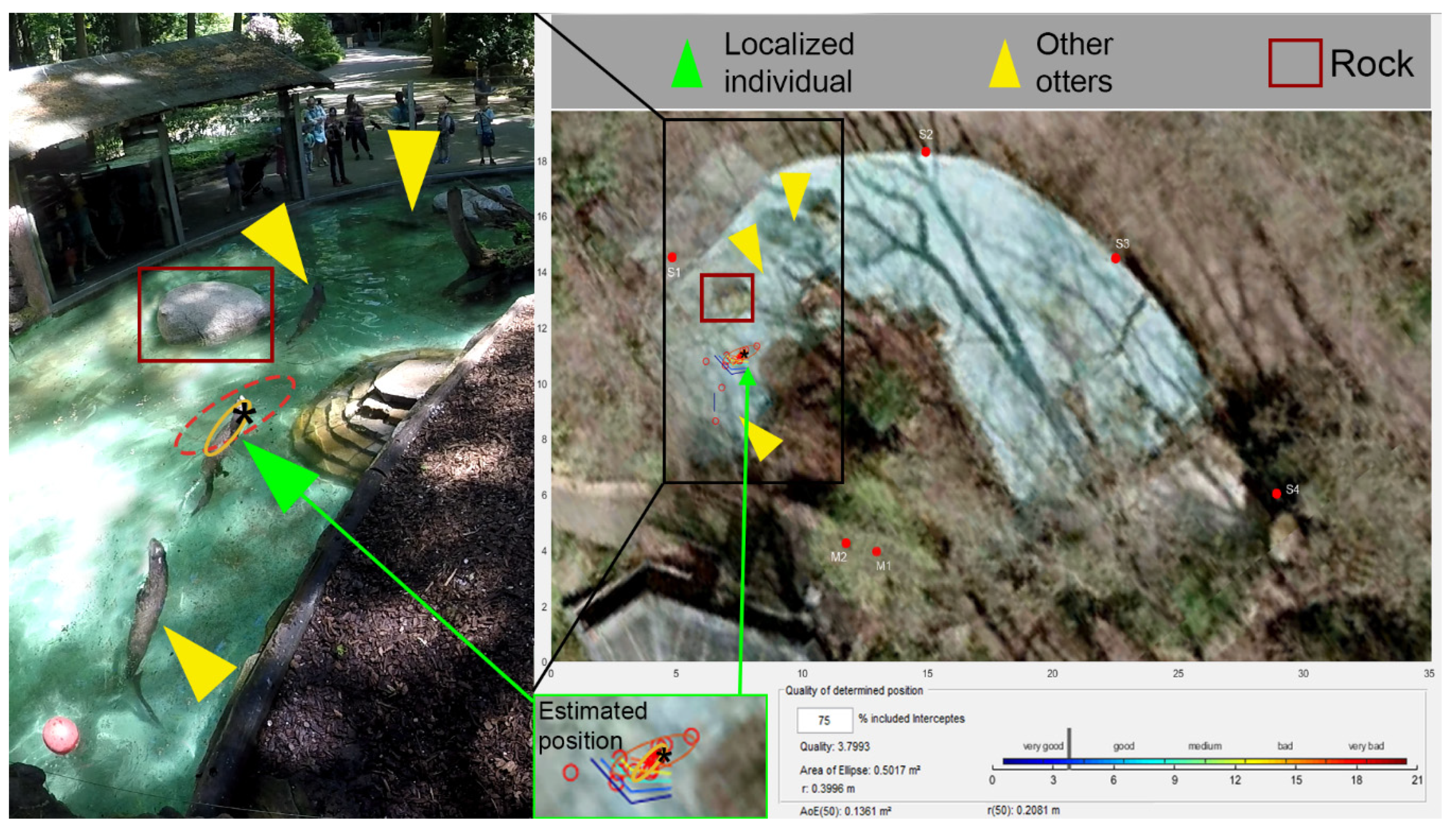
Example of sound localization using the software LASER in the giant otter enclosure. The left side of the figure shows the frame of the video recording at the time of the vocal utterance. The right side shows the result of the sound localization. The estimated position of the vocalizing animal is marked with a black asterisk. The area with the highest probability of location is enclosed with an orange ellipse (0.136 m2), which contains 50% of the intersections of the hyperboloids. The red dashed ellipse contains 75% of the intersections of the hyperboloids. In the video frame the corresponding individual at this position is marked with a green arrowhead. The positions of the remaining otters are marked with yellow arrowheads on the map as well as in the video frame. For orientation, a rock in the water is outlined with a red rectangle.
Figure 6.
Example of sound localization using the software LASER in the giant otter enclosure. The left side of the figure shows the frame of the video recording at the time of the vocal utterance. The right side shows the result of the sound localization. The estimated position of the vocalizing animal is marked with a black asterisk. The area with the highest probability of location is enclosed with an orange ellipse (0.136 m2), which contains 50% of the intersections of the hyperboloids. The red dashed ellipse contains 75% of the intersections of the hyperboloids. In the video frame the corresponding individual at this position is marked with a green arrowhead. The positions of the remaining otters are marked with yellow arrowheads on the map as well as in the video frame. For orientation, a rock in the water is outlined with a red rectangle.


Table 1.
Height at which the microphones were set up at the respective position (in meters).
| Microphone | M1 | M2 | M3 | M4 | M5 | M6 | M7 | M8 |
|---|---|---|---|---|---|---|---|---|
| Height (m) | 4.15 | 4.1 | 4.1 | 3.2 | 1.85 | 1.9 | 2 | 2.1 |
Publisher’s Note: MDPI stays neutral with regard to jurisdictional claims in published maps and institutional affiliations. |
© 2021 by the authors. Licensee MDPI, Basel, Switzerland. This article is an open access article distributed under the terms and conditions of the Creative Commons Attribution (CC BY) license (https://creativecommons.org/licenses/by/4.0/).
Share and Cite
MDPI and ACS Style
Schneider, S.; Dierkes, P.W. Localize Animal Sound Events Reliably (LASER): A New Software for Sound Localization in Zoos. J. Zool. Bot. Gard. 2021, 2, 146-163. https://0-doi-org.brum.beds.ac.uk/10.3390/jzbg2020011
AMA Style
Schneider S, Dierkes PW. Localize Animal Sound Events Reliably (LASER): A New Software for Sound Localization in Zoos. Journal of Zoological and Botanical Gardens. 2021; 2(2):146-163. https://0-doi-org.brum.beds.ac.uk/10.3390/jzbg2020011
Chicago/Turabian StyleSchneider, Sebastian, and Paul Wilhelm Dierkes. 2021. "Localize Animal Sound Events Reliably (LASER): A New Software for Sound Localization in Zoos" Journal of Zoological and Botanical Gardens 2, no. 2: 146-163. https://0-doi-org.brum.beds.ac.uk/10.3390/jzbg2020011