
Exploring the Sensitivity of Recurrent Neural Network Models for Forecasting Land Cover Change


Spatial Analysis and Modeling Laboratory, Department of Geography, Simon Fraser University, Burnaby, BC V5A1S6, Canada
*
Author to whom correspondence should be addressed.
Land 2021, 10(3), 282; https://0-doi-org.brum.beds.ac.uk/10.3390/land10030282
Submission received: 9 February 2021
/
Revised: 3 March 2021
/
Accepted: 8 March 2021
/
Published: 10 March 2021
(This article belongs to the Special Issue Deep Learning Algorithms for Land Use Change Detection)
Abstract
:Recurrent Neural Networks (RNNs), including Long Short-Term Memory (LSTM) architectures, have obtained successful outcomes in timeseries analysis tasks. While RNNs demonstrated favourable performance for Land Cover (LC) change analyses, few studies have explored or quantified the geospatial data characteristics required to utilize this method. Likewise, many studies utilize overall measures of accuracy rather than metrics accounting for the slow or sparse changes of LC that are typically observed. Therefore, the main objective of this study is to evaluate the performance of LSTM models for forecasting LC changes by conducting a sensitivity analysis involving hypothetical and real-world datasets. The intent of this assessment is to explore the implications of varying temporal resolutions and LC classes. Additionally, changing these input data characteristics impacts the number of timesteps and LC change rates provided to the respective models. Kappa variants are selected to explore the capacity of LSTM models for forecasting transitions or persistence of LC. Results demonstrate the adverse effects of coarser temporal resolutions and high LC class cardinality on method performance, despite method optimization techniques applied. This study suggests various characteristics of geospatial datasets that should be present before considering LSTM methods for LC change forecasting.
1. Introduction
Land Cover Change (LCC) is a dynamic process with spatial and temporal dependencies. The interactions within and between human and natural environmental systems propagate LCCs over space and time [1]. These local-level interactions give rise to patterns observed at global scales [2]. For instance, anthropogenic disturbances such as deforestation directly and indirectly induce increased CO2 levels and affect local weather changes, making LCC important to consider as global temperatures rise [3,4,5,6]. LCC research is significant to many disciplines such as geography, urban planning, environmental science, forestry, agriculture, and resource management [7,8,9].
Land changes have been previously modeled using methods that capture local-level interactions occurring over space and time. These include geographic automata approaches, comprised of Agent-Based Models (ABMs) and Cellular Automata (CA) [10]. For instance, encoded agents can capture decision-making processes of individuals or groups [11,12]. Such decisions have implications on the environment represented in an ABM. CAs have also been demonstrated to capture land change over time according to pre-defined transition rules across a regular [13,14,15] or irregular-grid environment [16]. Different types of ML models have also been used in conjunction with CA, including support vector machines [17,18], random forests [19], neural networks [20], and Markov models [21]. Another integration considered an ABM, a CA, and a system dynamics model to facilitate interactions across multiple scales that drive land changes [22]. However, limited knowledge of individuals or disaggregated system behaviours impose limits on what type of model can be used [23]. As such, data-driven methods may be used in situations where patterns and relationships driving land change are unknown.
Given the complexity of LCC, statistical learning approaches have been applied for analyses in this domain [24,25]. Earlier approaches include regression models that integrate field measurements alongside classified LC data [26]. Throughout the past decade, data-driven modeling methods usage has been rising with the unprecedented availability of data, the Big Data paradigm shift, and the escalating capacity of computational resources [27]. While Machine Learning (ML) algorithms automate pattern recognition with minimal manual interference, it is important to acknowledge that these techniques are deterministic approaches to modeling non-linear spatial processes. With increasing dimensionality and volume of modern datasets, ML algorithms typically perform with great efficacy. Several ML approaches previously applied for Land Cover (LC) classification and forecasting have included Neural Networks (NNs) [28], Decision Trees [24,29], Random Forests [24,30], and Support Vector Machines [24,31].
A subfield of ML characterized by NNs of increasing depth and breadth is called Deep Learning (DL). DL techniques facilitate automated learning of feature representations and have demonstrated ability to capture intricate, hierarchical relationships from a dataset [32]. A Recurrent Neural Network (RNN) is a type of NN suitable for sequential data. With internal memory allocated to each neuron, RNNs are useful for capturing dynamic, temporal dependencies [33]. RNNs, specifically the Long Short-Term Memory (LSTM) variation, have exhibited propitious performance in previous LCC analyses [25,34,35]. However, geospatial input data characteristics conducive to the success of LSTMs have not been fully studied. This motivates an investigation of the method’s response to varying geospatial data qualities by means of Sensitivity Analysis (SA).
SA is helpful for assessing the effects of geospatial input data properties on model outputs [36]. For example, SA approaches applied to ABMs [37] and CAs [38] have been considered. SA approaches were also employed for super-resolution LC mapping [39] and LCC modeling [40,41]. Furthermore, perturbations to inputs provided to a decision-tree modeling approach were explored with respect to overall test accuracy and the number of cells changed [42]. Prior studies involving ML techniques have also emphasized measuring a model’s capacity to forecast changed cells correctly [43]. Traditional NNs and DL approaches used for applications besides LCC have been explored for their sensitivity to input representations [44], introduction of noise [45], and input variables [46]. While extensive numbers of parameters and permutations characterize methods such as geographic automata and data-driven approaches, it is important to consider what characteristics of an inputted dataset are conducive to or impede the usefulness of a selected method.
This compels a study to assess the implications of changing geospatial input data properties on the performance of LSTM models and to evaluate their ability to forecast localized LCCs using a SA. Facets of LCC processes such as LCC rate, temporal variations, and local-scale processes are important to consider [47]. Previous work indicated that when considering four LC classes, the method performance was impacted by fast-changing phenomena [48]. However, it was unknown whether this trend persisted given LC datasets with increasing cardinality. As such, the impact of both varying temporal resolution and number of LC classes is explored in this work. This research considers LCC sequences extracted along the temporal dimension for each cell within various hypothetical and real-world datasets featuring different numbers of LC classes as input to LSTM models. Hypothetical datasets are first created and utilized to reconstruct real-world LCC scenarios occurring in localized study areas. By reducing the hypothetical data complexity for this study, it is intended to highlight trends in results generated. Experiments are then conducted on real-world data to observe if trends observed in the hypothetical data trials are similar. Given the increasing availability of multi-year LC datasets, it is important to better understand what properties should be present to use this data-driven sequential method. By exploring results obtained from applying LSTM modeling scenarios to hypothetical and real-world datasets, the aim is to guide future real-world data selection for potential use with the explored method. Similarly, this research work intends to help inform researchers who have already acquired geospatial data whether this method is appropriate given the temporal resolution, number of timesteps, number of classes, and rates of change characterizing their dataset.
To explore which data properties should exist to use this method, an SA is evaluated with a collection of incremental modeling scenarios involving a selection of Kappa metrics. The main objective of this research study is to explore and evaluate the impact of varying temporal resolution on LC changes forecasted using LSTM models and datasets featuring different numbers of classes. The metrics are selected for measuring these effects with respect to how well the respective modeling scenarios forecast changed cells, since LCC typically exhibits slow or scarce changes over time. The quantities of interest are the changed cells forecasted correctly by the model. It is hypothesized that performance of these sequential DL models will be impeded by low temporal resolutions, which feature shorter sequence lengths. Likewise, it is expected that greater LCC occurrences will ensure changes are captured better in all modeling scenarios applied to hypothetical and real-world datasets. It is also anticipated that experiments considering fewer unique classes will yield more favourable results.
2. Theoretical Background and Geospatial Applications of RNNs
Traditional feed-forward NN models utilize gradient-based learning methods to update model parameters as new inputs are provided. The goal is to determine an optimal set of network weights that allow the model to generalize to new data. Inputs are fed through the network, a cost function is evaluated, and an error term is computed using the result obtained from the output layer. Derivatives are computed with respect to each weight in the network using a process called backpropagation [49,50]. Backpropagation informs adjustments of network weight parameters with the intent of minimizing the error term.
RNNs are a type of Deep Neural Network (DNN) that are best suited for problems involving sequential data, including classification and forecasting of timeseries data. By introducing a recurrence relation to the standard feed-forward neuron, information from previous timesteps is propagated to inform future cell state changes and outputs. Traditional RNNs are a specialized variation of traditional neural network neurons that maintain and update a hidden state value. The hidden state enables a recurrent neuron to maintain information regarding previously observed data in a sequence to facilitate learning of temporal correlations [51]. However, RNN structures are impeded by a phenomenon called a “Vanishing Gradient” [52]. This occurrence inhibits the propagation of previous information and is caused by the inability to maintain gradients to backpropagate updates with respect to the error term. Gradients that are too small (vanishing) or too large (exploding) prevent any meaningful adjustments of network weights. This required alterations to the RNN architecture to handle long-term dependencies.
A notable architecture advancement of the RNN is called Long Short-Term Memory (LSTM), developed to solve the “Vanishing Gradient” problem [33]. This definition is characterized by the addition of memory cells to maintain information regarding previous states and gates to permit or prevent information to be stored within the memory cell. The idea was to maintain the error term to ensure the error signals were not lost due to the Vanishing Gradient problem [33]. To further improve the LSTM architecture, it was suggested that a forget gate be added to enable an LSTM to drop information that has been maintained if the contents are no longer of use [53]. Gates in a modern LSTM cell include an input gate, forget gate, output gate, and input modulation gate, which control how much information is permitted to propagate through the cell [25,35]. Explanations of the updates of an LSTM cell at timestep t when provided an input can be found at Donahue et al. [54].
RNNs have been used for classification and forecasting tasks in geospatial applications [9]. To apply RNNs to geospatial datasets, cell-wise (or pixel-wise) temporal sequences are provided as training data with a corresponding “training label” signifying the next data entry in the timeseries at the location being considered. Sauter et al. [55] utilized snow cover derived from MODIS satellite data with meteorological data to develop a snow depth forecasting system using an early RNN approach. More recently, an LSTM model called REFEREE [35] demonstrated the abilities of RNN for binary and multi-class LCC detection. The transfer learning scenario involved various study areas featuring urban, water, soil, and agriculture LCs. LSTMs have also been used to forecast sea ice concentration, with input sequences extracted along the temporal dimension for each cell in the raster dataset [56]. In addition, RNNs have proven effective in LC classification. Provided timeseries inputs consisting of 3- and 23-timesteps, an LSTM model showed improved performance over Random Forest and Support Vector Machine methods [25].
Though it is acknowledged that a multitude of RNN architectures and variants exist, LSTM has been selected for this study as the primary architecture to be evaluated for its capacity to model LCC. A prior study compared the performance of LSTM and its variants, demonstrating insignificant improvements obtained over the traditional LSTM architecture in applications such as handwriting recognition and music modeling [57]. It was also demonstrated that traditional LSTM networks have the capacity to reliably obtain improved performance versus its simplified variant, the Gated Recurrent Unit (GRU) [58], in large-scale “neural machine translation” tasks [59]. Stacked LSTMs have also been previously explored for LCC with respect to varying temporal resolutions, rates of LCC, and errors arising from classification procedures [48]. Considering four LC classes in experiments, the results indicated the importance of finer temporal resolutions and the inclusion of more timesteps to increase the capacity of this method to forecast LCCs.
While previous studies have demonstrated the effectiveness of RNNs and variants for geospatial applications, the performance of these methods with respect to geospatial data properties remains an open problem. Therefore, this research study explores the repercussions of temporal resolution and LC class count present in the input dataset. Changing these characteristics alters the sequence length and rates of LCCs provided as input to the LSTM models. Using SA applied to three modeling scenarios considering hypothetical and real-world data, the goal of this study is to explore the response of RNNs to varying geospatial data inputs.
3. Materials and Methods
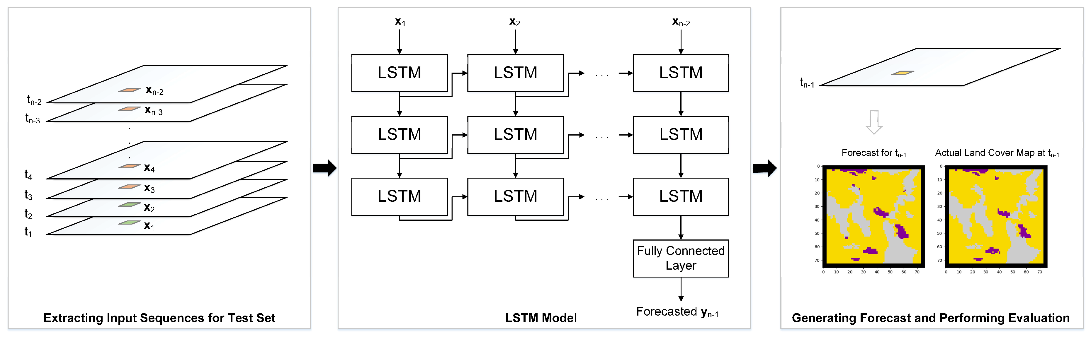
The systematic assessment of RNN, specifically LSTM, involves modeling scenarios established to represent a typical development progression. The model response to changing geospatial input is assessed in each scenario. This involves changing the temporal resolution parameter to the next smallest increment possible while maintaining the comparison of the same LC data layer across all scenarios. For each change of temporal resolution, the experiments are performed on one of the different datasets containing a different number of classes. The aim is to observe if there are trends in model response on changed temporal resolution despite model optimizations. An overview of the end-to-end methodology used to generate forecasted maps in each scenario is shown in Figure 1.
3.1. RNN Model Development
A baseline RNN model undergoes optimizations to create three modeling scenarios. In this work, a stacked LSTM model comprised of three layers and 32 neurons per layer forms the baseline RNN model. This is because stacked DL models have proven their ability to learn increasingly complex relationships [60,61]. The input layer is compatible with the one-hot encoded sequences. One-hot encoding involves converting LC class labels to vectors containing zeroes and a single non-zero value (1) at the index corresponding to the class ID [62]. Each input sequence is a matrix of N × M dimensions corresponding to respective cells across the study area, where N denotes the number of timesteps and M denotes the number of possible categories represented by the one-hot encoded vector. The output layer of the respective models produces an M × 1 vector containing the probabilities of each LC class forecasted to occur at the next timestep for a single cell. The position in the output vector featuring the highest probability is selected, with the position in the vector corresponding to the forecasted class label.
The configuration of parameters for the baseline RNN model includes pre-set components as well as iteratively selected hyperparameters (parameters that are set a priori to aid the model in achieving the “statistical generalization”). Hyperparameters set before initiating training procedures affect optimization of the model’s internal parameters, thus influencing the quality of the model. The number of internal model parameters affected by the hyperparameters selected prior to model training is 24,567. Using a grid search approach, two model hyperparameters, the number of epochs and batch size, were determined for the respective models constructed with respect to each dataset [56]. The number of epochs refers to how many times the entire dataset is passed through the network and batch size refers to how many data points are considered when computing the gradient prior to each update of the model’s internal parameters (weights and biases). The Adam optimization algorithm [63] is used instead of the traditional stochastic gradient descent approach due to its proven success and its robustness to model hyperparameters. Categorical cross-entropy is utilized as the objective function to accommodate the multi-class data sequences. The Softmax activation function [49] was employed for the output layer to produce a vector of probabilities corresponding to each class label [25]. This activation function is commonly used in models designed for multi-class classification and forecasting tasks [49]. Models were implemented using the Python programming language (v3.6.5) [64] and the Keras API (v2.2.0) [65]. The Keras API assists developers in prototyping ML and DL models while providing an interface to the extensive functionality of Google’s TensorFlow (v1.8.0) [65]. TensorFlow is an open-source ML framework that provides advanced features to construct and fine-tune data-driven models [66]. Model development took place on a workstation equipped with an NVIDIA GeForce GTX 1080 Ti GPU.
3.1.1. Modeling Scenarios
Using the baseline stacked RNN model described in Section 3.1, modeling scenarios were created to assess method sensitivity to varying input data characteristics. These include (1) a deterministic baseline, (2) a stochastic scenario, and (3) a regularized stochastic scenario, which are referred to as Model A, B, and C, respectively. By emulating a conventional DL model development pathway, it is intended to reveal whether resulting metrics obtained exhibit trends that endure as models are optimized. The scenarios ensure results are not unique to a specific configuration, as there are infinite arrangements and numerous model optimization techniques that have proven to improve results various applications [67].
The deterministic baseline modeling scenario (Model A) provides a foundation for subsequent models. The structure and parameters of this model are equivalent to the baseline RNN model described in Section 3.1. However, in Model A, a random seed is used instead of allowing different network weight initializations for each run. This is done to assure results are reproducible given the same set of input parameters over repeated tests to form a “deterministic baseline” by which to compare the subsequently optimized models.
Next, the stochastic scenario (Model B) uses “true” random weight initialization with the removal of the random seed. Model B has the same structure as Model A, with the only difference being that initial weights for each run are set randomly. Reintroducing stochastic weight initialization potentially leads to improved performance, with sets of initial weights affecting the attainment of optimal model parameters during the batch gradient descent procedure [68].
Finally, a regularized stochastic scenario (Model C) is developed to improve generalization and to prevent overfitting. The baseline LSTM model as described in Section 3.1 is modified by applying dropout regularization between each of the LSTM layers and the final output layer. The dropout regularization method forces a percentage of neurons to be ignored [69]. Dropout has been used in previous work involving geospatial data inputs extracted along the temporal dimension, informing a dropout factor of 0.5 [32]. This means that the probability that a neuron is “dropped” is 50% [69]. When a neuron is “dropped”, input and output connections to the neuron are also ignored. In addition to dropout regularization, Model C continues to use the random initialization of weight parameters, as was characteristic to Model B.
3.2. Sensitivity Analysis
To ensure each modeling scenario was evaluated equally, a collection of test cases was designed. This research study uses a local SA technique in which one input parameter or variable is adjusted at a time to explore how small changes to model inputs affects the model outputs [40,70]. The inputted data sequences provided to train an LSTM are important because these models exhibit sensitivities to sequential order, with each timestep or data element considered one at a time [71]. If data are perturbed in the sequence, a representation learned could be completely altered. In previous studies, focus was placed on observing changes to model behaviour as a result of initial inputs for other modeling approaches [72]. For instance, inputted data have proven impactful on the performance of modeling approaches because changes occurring within a system are highly dependent on previous states, originating from initial conditions [73]. Therefore, this motivates the use of a local sensitivity analysis or “one-at-a-time” approach to be considered for this research study.
For each synthetic dataset, for each temporal resolution, and for each modeling scenario, a grid search of hyperparameter space was conducted, producing new models and results at each iteration. Trained models were then tested, generating a forecasted map output for the next unobserved timestep. While outputs of all test case combinations were logged, the best performing models were selected based on their ability to forecast changed cells using the test set. Forecasted and reference maps were compared using a variety of metrics to assess the method’s sensitivity to varying input data characteristics. In previous studies, overall accuracy and traditional Kappa metrics have been used when comparing forecasted and reference LC maps to reason about a model’s usefulness [74]. For instance, SA methods have involved measuring a model’s forecasting ability by comparing forecasted maps with reference maps and via Kappa indices and Receiver Operating Characteristic (ROC) statistics [75]. While overall accuracy, the traditional Kappa measure, and other overall summary measures provide a means to quantify a model’s performance based on model output, these typical metrics do not suffice for this study where the focus is to understand how well the method forecasts LC changes, due to the slowness or scarcity of LCCs. This motivates the use of accuracy measures considering changed cells and variations of the traditional Kappa metric that likewise differentiate transitions or persistence of LC.
In this research study, accuracy with respect to the number of changed cells and a suite of Kappa metrics were utilized (Table 1). Previous geospatial applications of RNNs have also relied on traditional Kappa statistics [25,35,76], including Kappa, KHistogram, and KLocation [74]. The Kappa metric provides a measurement of agreement between two maps being compared, while KHistogram considers the quantity of similarities between the two maps being compared [77]. KLocation is another a measurement of agreement based on similarity of location for each class between two maps compared [74]. However, traditional Kappa measures provide overall values of quantity-based agreement without detail regarding categories or types of cells that are in disagreement [78]. Therefore, to evaluate the method’s ability to forecast changes, KSimulation, KTransition, and KTranslocation have also been selected [74,77]. These measures are considered “three-map comparisons,” requiring a reference map, a reference map pertaining to the previous timestep, and the forecasted map [79]. The formulation of the KSimulation, KTransition, and KTranslocation equations dismisses the effects of persistent cells, enhancing assessment of the method’s ability to simulate changed cells [77]. KSimulation is a measure of agreement for changed cells present in a reference and simulated map. KTransition is a measure of agreement between the number of transitions occurring for each class between a reference and simulated map. Lastly, KTranslocation or “Kappa transition location” provides a measure of agreement based on the similarity of location for transitioned cells in each LC class.
4. Geospatial Datasets and Pre-Processing
4.1. Hypothetical Data
The first set of experiments conducted consider hypothetical data. Hypothetical datasets are commonly used in geosimulation modeling [37,80] and can be used to regulate geospatial input characteristics to assess method response to changing inputs [81]. In addition, using synthetic small-area datasets enables localized analyses and reduced computation time to perform evaluations [82]. In this study, synthetic LC datasets were created to control the number of unique LC classes and rates of change.
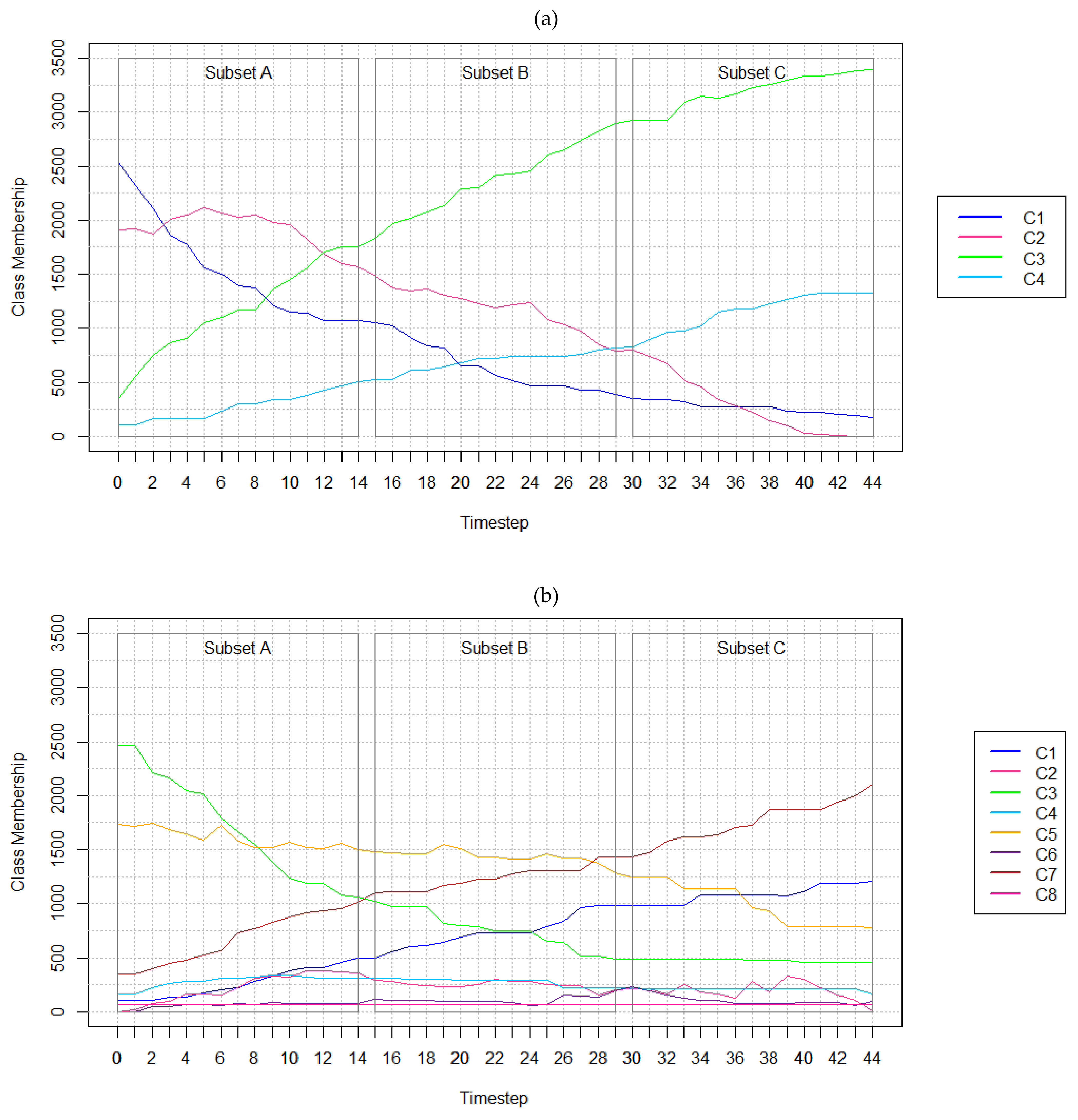
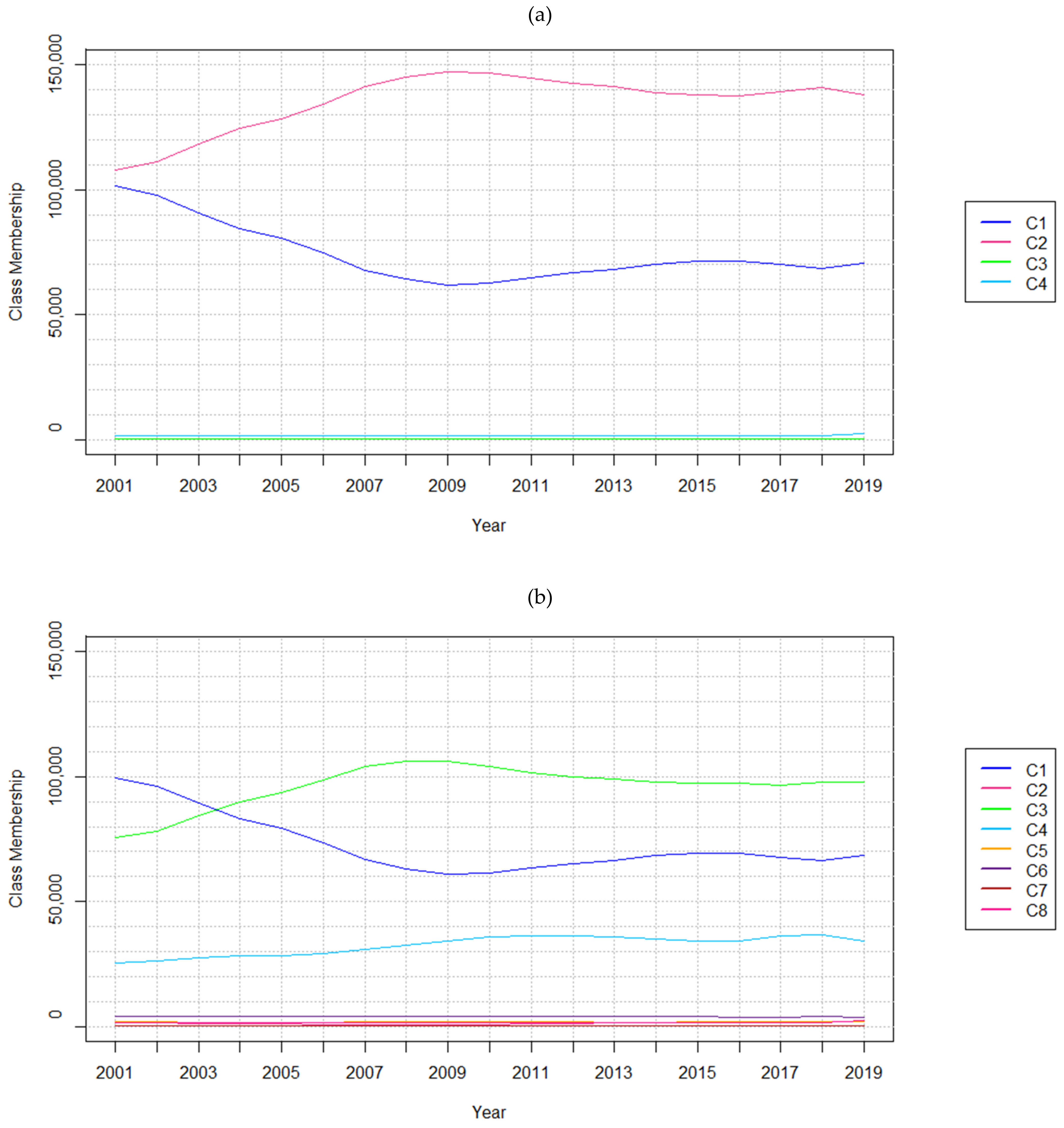
The three datasets developed feature 4, 8, and 16 LC classes, respectively (Table 2). The LC classes composing the respective datasets have been named as per real-world classes featured in Homer et al. [83] and Sulla-Menashe and Friedl [84]. The synthetic datasets have been generated using Esri’s ArcGIS Pro (v2.4.0) in order to control LC changes to emulate or exaggerate real-world scenarios [85]. That is, the LC classes have been specified to emerge, grow, or dissipate over time. For instance, in the four-class dataset, forest, and cropland are shown to transition to low and high intensity developments (Table 3, Figure 2). Class membership refers to how many cells belong to each land cover class at each timestep.
Each dataset has identical dimensions, temporal resolution, and number of timesteps. Datasets feature 76 × 76 cells with 25-meter spatial resolution. A 3-cell buffer is considered around the entire study area to mitigate edge effects. Edge effects are a conceptual issue requiring consideration when dealing with geospatial data [86]. This means that points outside of a geographic dataset will be influenced by points surrounding it. Thus, cells towards the middle of the study area are likely to be increasingly similar, while cells closer to the edges will be influenced by nearby phenomena and influences that are excluded from the dataset. This results in a working study area of 70 × 70 cells. These dimensions were chosen to expedite the evaluation processes, as small models (where breadth and depth are relatively small) can be typically expected to fit to small-scale datasets [68]. Each full dataset features 45 years with one-year temporal resolution.
The number of cells belonging to each LC class at each timestep are shown in Table 3 and Figure 2. Test cases considering all 45 years, including timesteps t0 to t44, are referred to as full sequence tests. Five full sequence tests feature five different temporal resolutions (1, 2, 4, 11, and 22-year) that ensured t0 and t44 were included in all cases. This guaranteed equal comparisons of forecasts for t44. Shorter sequence lengths were tested by utilizing subsets of the 45-year datasets available (Figure 2). Subsets contain 15 timesteps each, where Subset A includes t0 to t14, Subset B includes t15 to t29, and Subset C includes t30 to t44. The three 15-year test cases defined feature one, two, and seven-year temporal resolutions.
4.2. Real-World Data
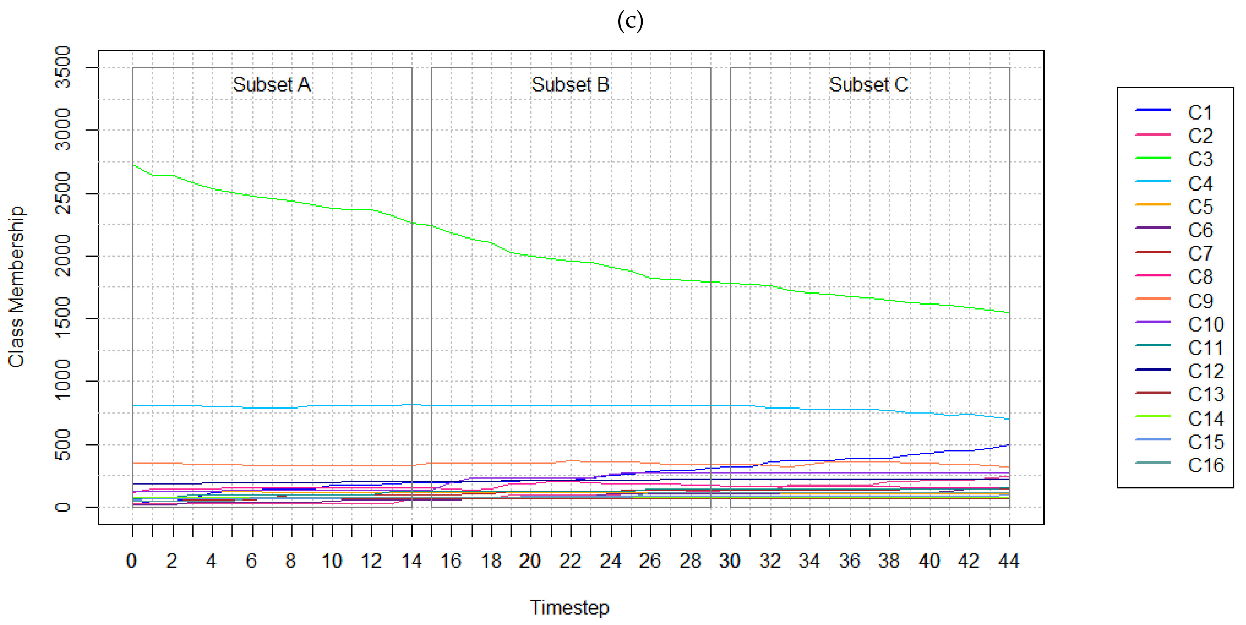
The next set of experiments considers real-world data obtained from the “MODIS Terra+Aqua Combined Land Cover product” [87]. The dataset features annual global land cover data with a 500-meter spatial resolution for years 2001 to 2019. The land cover layers used in the experiments are from the subset titled “Land Cover Type 1: Annual International Geosphere-Biosphere Programme (IGBP) classification.” The classification system makes available 17 unique LC classes. This study considers a subset of this data, focusing on the Thompson-Nicola Regional District in the province of British Columbia, Canada (Figure 3), obtained from the BC Data Catalogue [88]. The largest city in this district is Kamloops, with a population of 90,280 people as of 2016 [89]. This city is indicated in Figure 3d and is the focus for qualitative map outputs produced in the modeling scenarios. This region was selected for the exhibited diversity in LC, with 15 of the 17 possible LC classes from the MODIS data present in this region.
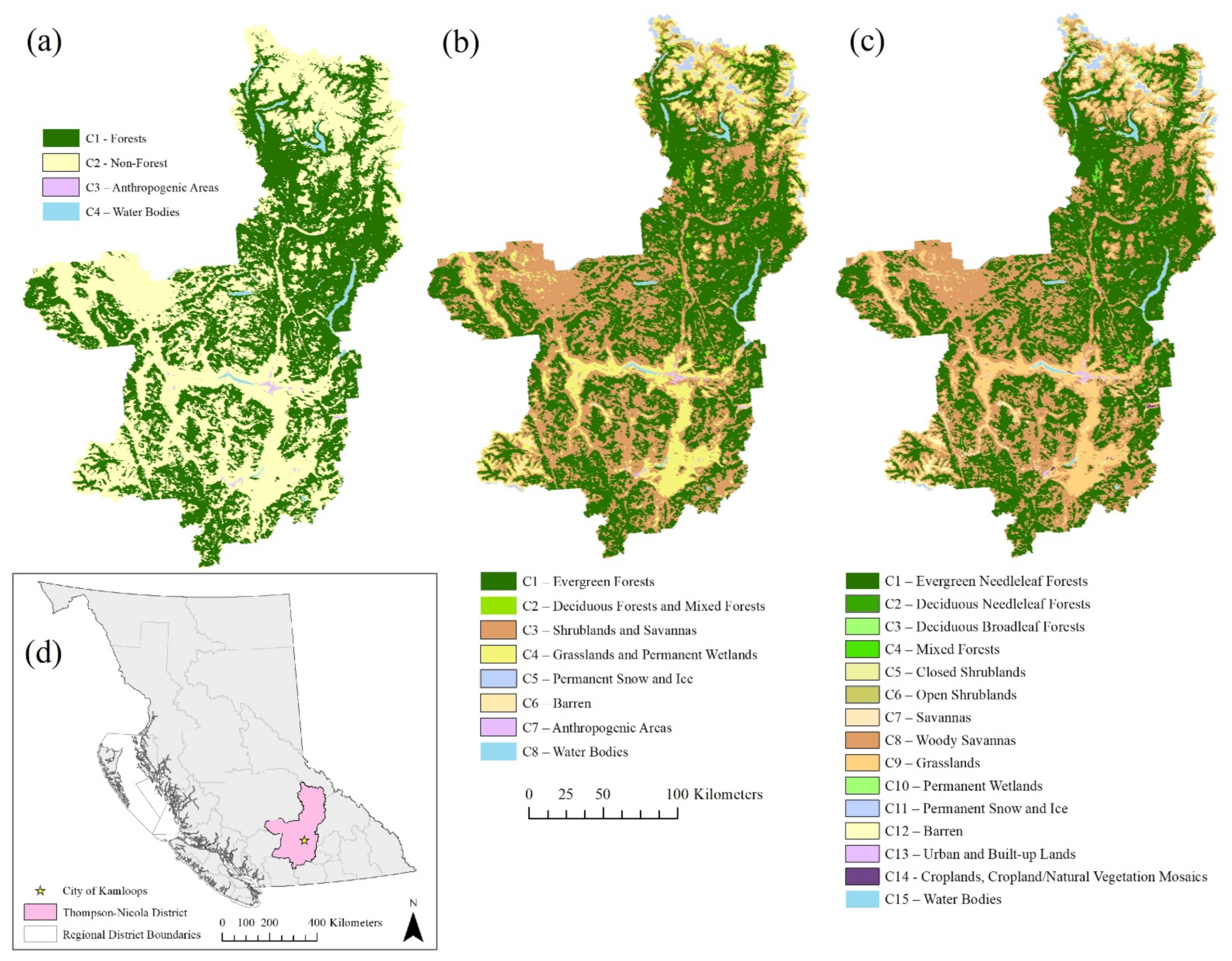
After clipping the MODIS LC data to the regional district boundary, three datasets were developed to feature 4, 8, and 15 LC classes, respectively (Table 4). This involved reclassifying the original data featuring 15 classes aggregated to 8 classes first, then to 4 classes (Figure 4). Within this real-world LC dataset, rates of change increase and decrease according to not only anthropogenic and environmental disturbances but are also affected by classification errors. These changes are reflected in the increases and decreases of cells belonging to each class for each of the 19 years considered for these experiments (Table 5, Figure 4).
The 4, 8, and 15 LC class datasets have identical dimensions, temporal resolution, and number of timesteps. Datasets feature 1847 × 832 columns and rows (including the edge cells) with 500-meter spatial resolution. A 3-cell buffer is considered around the entire study area to mitigate edge effects for reasons described in Section 4.1. This results in a working study area of 211,514 cells available per data layer. Each full dataset features 19 years with one-year temporal resolution. Five full sequence tests feature five different temporal resolutions, including the original temporal resolution (one, two, three, six, and nine years). Each sequence includes both t2001 to t2019 to facilitate comparisons of forecasts for t2019. Using all 19 years available was determined to explore if trends found using these real-world datasets exhibited similar tendencies to those found in the variety of 15-year subset experiments developed using the hypothetical data while not discarding four of the available years.
4.3. Creating the Training and Test Sets
Input sequences are extracted from the synthetic datasets and real-world at each cell along the temporal dimension according to the specified temporal resolution. The sliding temporal window approach for establishing training and test sets is used [32]. An input sequence in the training set is denoted as (x0, x1, x2, …, xT-3), while the target LC class is denoted by (yT-2). Input sequences in the test set are denoted as (x1, x2, x3, …, xT-2), while the target LC class is denoted by (yT-1). Each (xT-N-1) and (yT-N), where N = 1 or N = 2, are one-hot encoded vectors representing the classes at each cell at each timestep. The data layers used in the model training and testing phases for the experiments involving real-world data has been shown in Table 6.
Accommodating imbalanced datasets is an open issue for ML and DL methods [90]. For geospatial applications, tactics such as random sampling may omit classes that are underrepresented in the dataset [91]. Previous studies have also considered using fewer unique classes to increase the number of training samples [22]. Given the disproportionate percentages of persistent versus changed cells in LC datasets, a balanced sampling strategy was used following procedures stated in previous works [43]. To balance the training sets, it was first determined if a change occurred in a training input sequence. If a change occurred, the sequence was marked as “changed” (otherwise “persistent”). If the number of sequences marked “changed” exceeded those marked as “persistent,” the entire training set was considered. Conversely, if more sequences were “persistent,” then equal counts of “changed” and “persistent” cells were sampled at random according to the original distribution. This means that the number of training samples available for each of the datasets and for each of the respective classes differs according to the number of changes that occurred to uphold the balanced sampling strategy. For instance, fewer training data are possible for the 15- or 16-class datasets to ensure all samples are proportionally represented.
5. Results
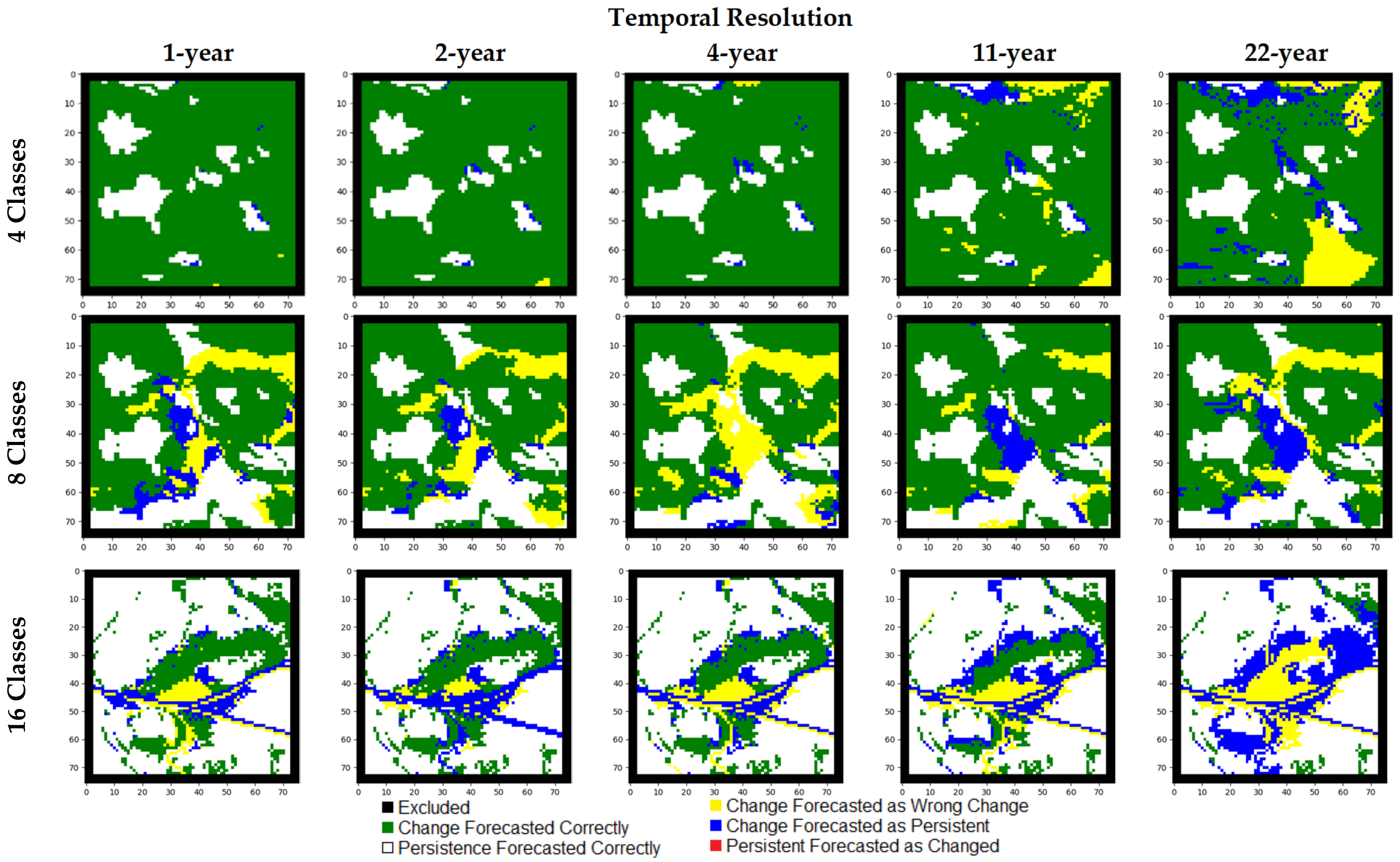
All modeling scenarios (A, B, and C) were run to generate results using the hypothetical and real-world datasets. This means that one run of a modeling scenario for the hypothetical datasets considers one of the 4, 8, or 16 class datasets, one of the full sequence or subset sequences, one of the temporal resolutions, and varying numbers of epochs to obtain one model and subsequent output. Considering the real-world datasets, each experiment considered one of the 4, 8, or 15 class datasets, one of the temporal resolutions, and varying numbers of epochs to obtain one model and the respective output. For each of the outputs generated by the respective models trained on either the hypothetical or real-world datasets, the various measures such as accuracy of changed cells and the suite of Kappa measures were computed. Additional to map comparison metrics, qualitative outputs were also produced for each model evaluation. These include simulation maps and maps featuring misses produced in the forecast. Overall, it was found that results from all three modeling scenarios were similar. Consequently, the results have been indicated by the regularized stochastic scenario (Model C) to explore the effects of temporal resolution and LC class cardinality on model performance.
5.1. Results of Experiments with Hypothetical Data
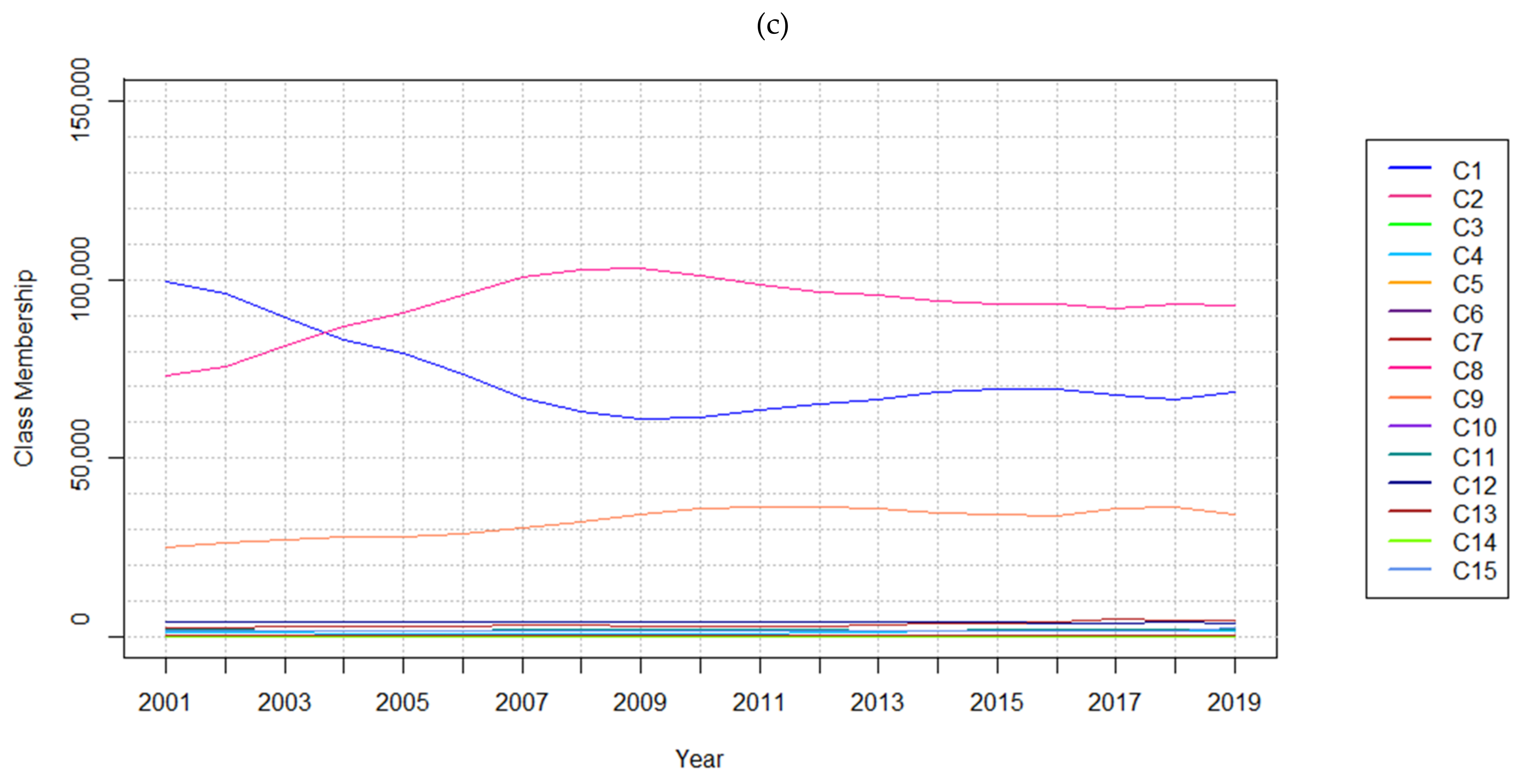
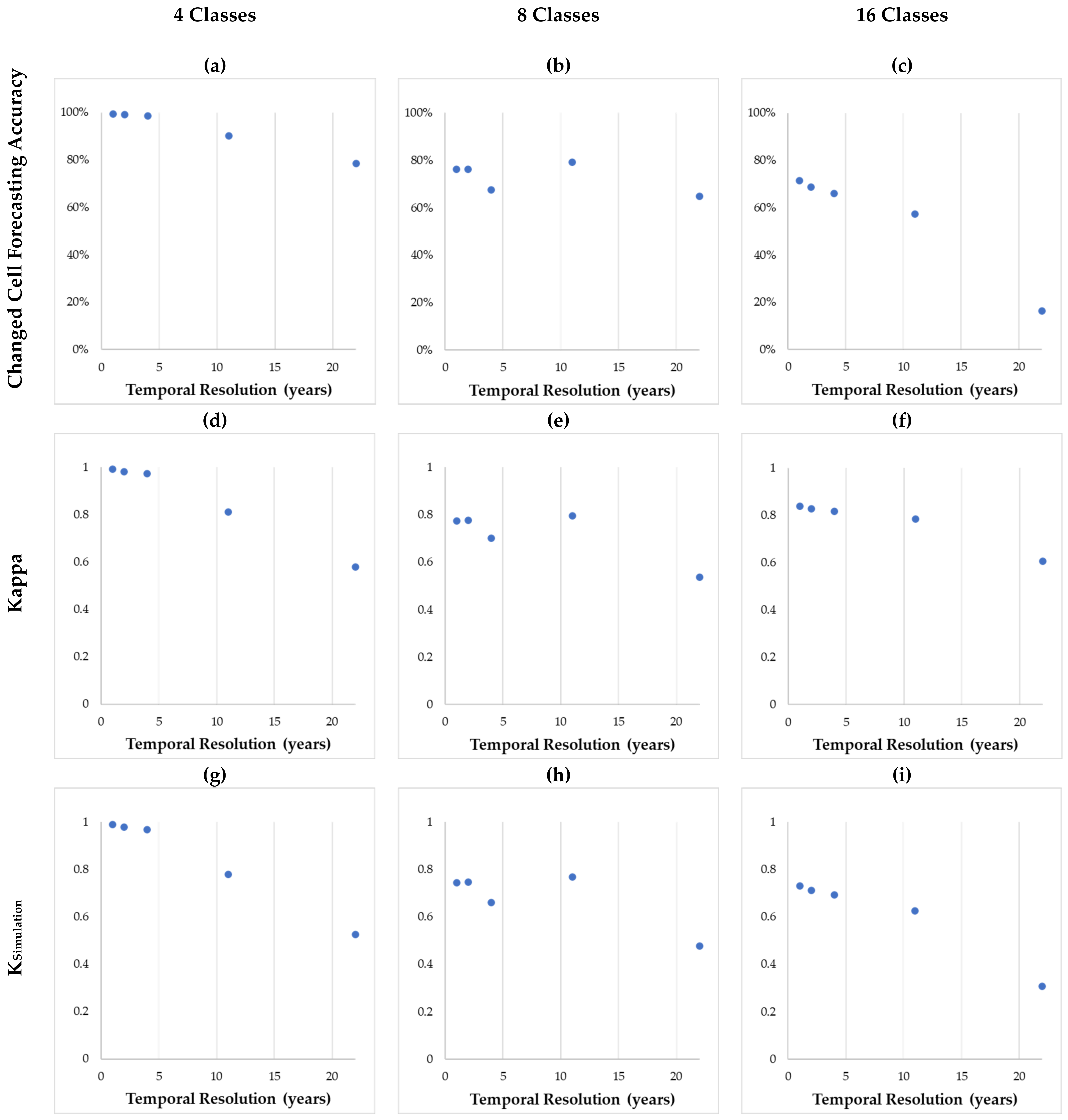
The results for full sequence tests featuring 45 years indicate models perform better with finer temporal resolutions (Table 7, Figure 5). Kappa, KHistogram, KSimulation, and KTransition measures exhibited distinct decreases as temporal resolution becomes coarser (i.e., fewer data layers) and as the number of classes increases. As the number of classes characterizing the study area increases, the number of errors in the forecasted map increase, demonstrated in Figure 6. The KSimulation measures decrease as temporal resolution becomes coarser and cardinality increases. For instance, KSimulation measures obtained using one-year temporal resolution data with 4, 8, and 16 LC classes are 0.99, 0.74, and 0.73, respectively. In almost all configurations, high agreements of persistent cells within the reference and forecasted map outputs were achieved. Simulation maps using the full sequence datasets are depicted in Figure 7.
The results for 15-year sequence tests show the KSimulation and KTransition metrics exhibiting sharp decreases as temporal resolution becomes coarser (Table 8, Table 9 and Table 10). With respect to the number of LC changes occurring, the overall map comparison metrics including Kappa, KHistogram, and KLocation are typically higher when the number of LC changes is lower. As the number of changed cells increases, these measures of map agreement decrease. It is also observed that these shorter sequence lengths used for input to the sequential models result in lower performance metrics than in the 45-year sequence tests in most cases. Results obtained using the 15-year sequences have been shown in Table 8, Table 9 and Table 10.
5.2. Results of Experiments with Real-world Data
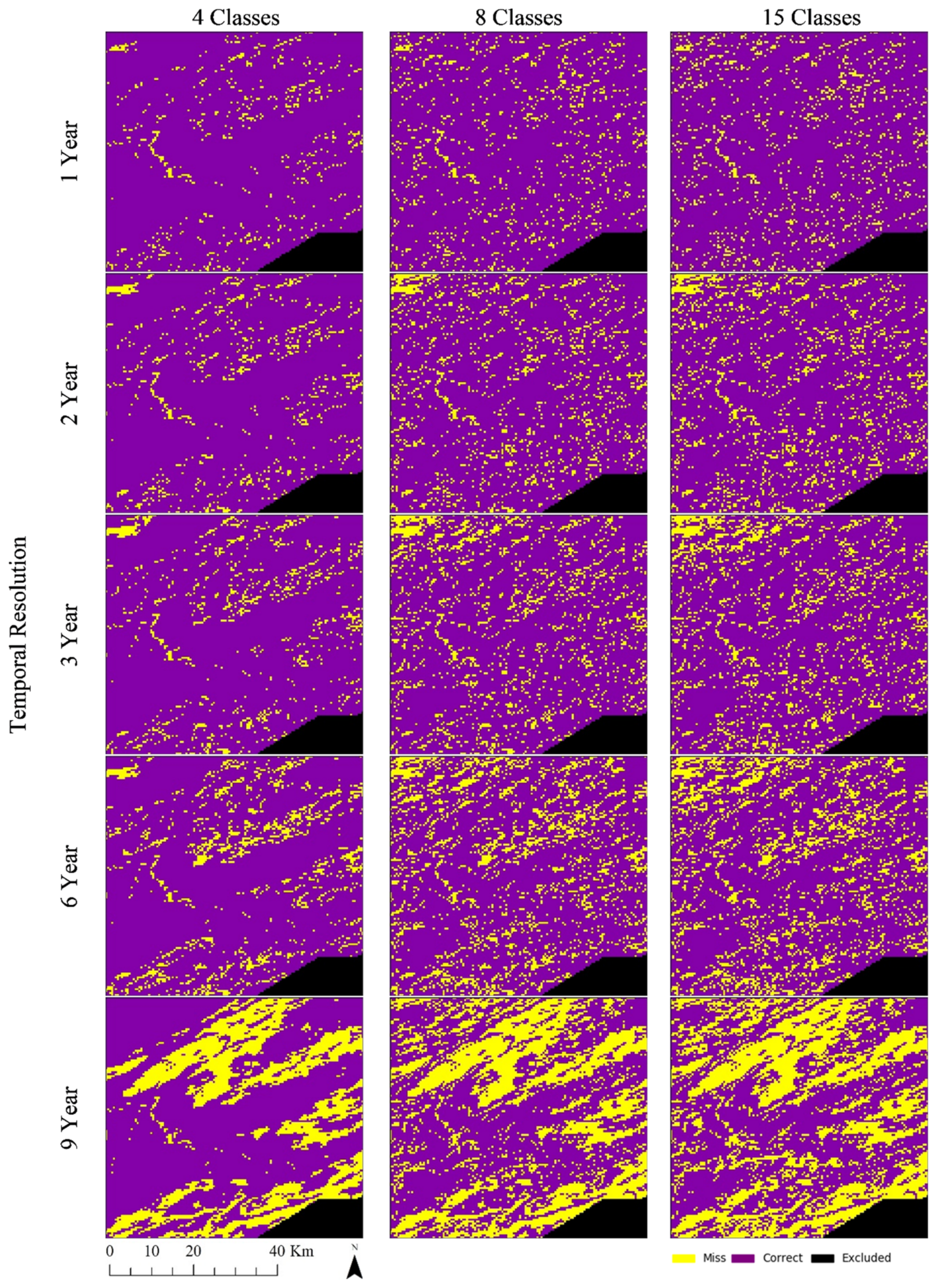
The results of the real-world data experiments considering each of the respective classes are shown in Table 11. All measures exhibited decreases as temporal resolution became coarser, except for the changed cell forecasting accuracy and KLocation measures produced using the four-class dataset as input. Likewise, when the number of LC classes increases, it is observed that the capacity of the models to forecast changed cells decreases. This is observed in the error maps focused on the City of Kamloops (Figure 8). The increasing number of errors in changed or persistent cells is reflected partially in the traditional Kappa metric, showing the agreement between the simulated and reference maps slightly decreasing from approximately 0.91 for the four-class dataset to 0.88 for the 15-class dataset. Larger differences between these two are exhibited in the KSimulation measure, indicating a greater presence of errors attributed to changed cells in the 15-class dataset as temporal resolution becomes coarser. The simulation maps focused on the City of Kamloops demonstrate this aspect of the outputs, showing an increasing number of cells that wrongly changed or remained persistent as the temporal resolution increases (Figure 9). While the KTransition measure indicates a high agreement of the quantity of transitions in each of the outcomes, the KTranslocation measure indicates that such transitions did not meet quite as high agreement of correct locations for these forecasted LC transitions. This is the case across all temporal resolution options except for those considering the nine-year temporal resolution.
6. Discussion
The aim of this research study was to explore the implications of varying temporal resolutions and LC classes. When analyzing results obtained from the SA conducted using the hypothetical and real-world datasets, it was observed that the methods are highly affected by temporal resolution. For instance, models trained on the hypothetical data performed better with finer temporal resolutions in most test cases. Changes that appear over coarser resolutions may appear more abrupt, impacting model performance. Considering the real-world datasets, the number of persistent cells incorrectly forecasted as changed also exhibits a sharp increase when considering nine-year temporal resolution data. This type of error is attributed to the observed class membership changing more rapidly from 2001 to 2010, as shown in Figure 4. The model would not have been provided sufficient data to forecast that the rapid changes had ceased from 2010 to 2019, a consequence of the sampling strategy used to form the training datasets.
In addition, the hypothetical scenario features no cells that transition back to a previous class. However, the real-world dataset features many cells that transition back to a previous class because of anthropogenic or environmental disturbances or classification errors. This is exacerbated by reclassification procedures applied to aggregate the original 15-class dataset. As such, the vast LC changes attributed to temporal resolution and increasing LC class cardinality are expected. LCC processes typically occur gradually over long periods of time and finer temporal resolutions preserve more detail. Thus, finer temporal resolutions are typically associated with higher changed cell forecasting accuracy.
Using one input feature with one input label for training and testing sequences, respectively, produced poor performing models for the respective datasets, aligning with the initial assumptions. This response to using the coarsest resolution indicates this type of model may not be appropriate for geospatial input datasets featuring only three timesteps available for training and testing. Using finer temporal resolutions with more timesteps produced the best results. Datasets with higher rates of change or variability also appeared to benefit from finer temporal resolutions. For example, the tests conducted considering the 19-year datasets show that despite rapid changes occurring between 2001 to 2010 for the Evergreen Needleleaf Forest and Woody Savanna LC classes, the models could still forecast changed cells with approximately 83% accuracy when using finer temporal resolutions (Table 11). An exception to this trend is shown in Table 8, where the four-class, 15-year hypothetical dataset including timesteps 0 to 14 is considered. Abrupt changes occurring between each timestep from timesteps 0 to 14 are expected to have impacted performance metrics. That is, considering the four-class synthetic dataset at two-year temporal resolution, cell transition rates are observed as less erratic. This further exemplifies the method’s sensitivity to increased or inconsistent rates of LCC.
Results showed that increasing sequence length improved a model’s capacity to forecast changes. For example, as the hypothetical data input sequence length decreased, models exhibited poorer performance. This is indicated by the overall map comparison metrics including Kappa, KHistogram, and KLocation. In cases where the smallest hypothetical data sequence lengths are used in both 45-year and 15-year test cases, KSimulation and KTransition indicate that models are hindered from learning LCCs. No model trained on the 15-year, four-class datasets exceeded performance measures of models trained on all 45 timesteps with one- and two-year resolution, indicating improved performance can be attributed to greater sequence length. This aligns with the experimental results conveyed by Ienco et al. [25], where outcomes obtained with a dataset featuring a greater number of timesteps consistently exceeded performance measures computed with respect to the dataset featuring fewer timesteps.
Overall, the four-class dataset was associated with the best performance metrics of all the tests conducted using the hypothetical and real-world datasets. This confirms the initial assumption that fewer unique classes would have a positive impact on the model outcomes. The SA indicates that dataset cardinality also affects method performance. Considering the hypothetical 16-class dataset, low accuracies were obtained when forecasting changed cells. Finer temporal resolutions and increased sequence lengths also improved model performance as LC cardinality increased. The four-class dataset was associated with models that forecasted LC transitions with greater accuracy. Considering the real-world 15-class dataset, changed cell forecasting accuracies produced differed less vastly from the four and eight-class data experiments. However, the capacity of the models to forecast changed cells decreased more rapidly as the temporal resolution became coarser despite model optimizations described in Section 3.1.1. This is attributed to the greater number of classes exhibiting changes that are not captured in detail using the coarser resolution. The results correspond with those communicated by Sun et al. [92], which indicated that experiments conducted using all classes yielded lesser accuracies versus those obtained with a fewer number of classes. It might also be observed as a repercussion of the potential decreasing sample size per class as the sampling strategy used to form the training datasets is upheld. This may lead to undersampling in cases where there are more classes, which can remove potentially important training samples [90].
Contrary to initial expectations, the SA demonstrated that the LSTM models were most effective when rates of LCC were more gradual. This coincides with the findings of Chi and Kim [56], where it was found that increased melting of sea ice in summer months impeded their LSTM model forecasts. The hypothetical 16-class subsets where few changes occurred enabled models to obtain improved performance measures despite high cardinality. As the number of changes increased, model performance suffered, especially when using coarse temporal resolutions and when considering the hypothetical 16-class dataset. This was also observed in results produced with the real-world dataset featuring 15 classes. With coarser temporal resolutions, the 15-class dataset experiments demonstrated decreasing performance observed in all metrics. The less dramatic decrements of performance measures observed considering the real-world dataset versus those obtained using the 16-class hypothetical dataset may be attributed to the larger dataset available.
While overfitting to smaller datasets may be an issue, many of the overall trends observed across the hypothetical and real-world datasets were present in both sets of results. Results of this SA correspond to previous findings indicating that the number of classes undergoing changes and coarser temporal resolutions were detrimental to the method’s performance [48]. Overall, cells featuring persistent LC were typically forecasted correctly with fine temporal resolutions across hypothetical and real-world experiments. This indicates that modifications or an alternate approach to the sampling strategy procedure used in this research study should be considered to obtain improved results that are less biased toward the majority class of cells, whether they be persistent or rapidly changing.
7. Conclusions
The primary objective of this study was to examine the impact of temporal resolutions and the number of LC classes on LSTM model performance via a SA. This SA involved measures focused on quantifying the capacity of the method to forecast LC changes explicitly rather than focus on overall accuracy measures as reported. These experiments were conducted using hypothetical and real-world datasets to observe whether trends persisted across experiments. The systematic SA identified similar responses across Modeling Scenarios A, B, and C, with inconsequential differences between them. As a result, measures reported and explored were those obtained from the optimized Model C (described in Section 3.1.1) for this research study. Overall, similar trends in results were obtained with respect to the hypothetical and real-world datasets.
Results indicated that LSTM models are sensitive to the change of temporal resolution in all experiments conducted by forecasting different LCC outcomes as model outputs. These experiments included datasets featuring a different number of classes in both the hypothetical and real-world datasets and resulted in the same conclusions. Based on this sensitivity analysis, it was found that LSTM models perform best when datasets feature finer temporal resolution and fewer LC classes. Based on these results, it would be advisable to aggregate LC classes in cases where only coarser temporal resolution LC data is available. These findings also imply that if more input data layers were given at the shortest temporal intervals possible, this would enable LSTM models to be used for more gradual LCCs forecasting. Similarly, this study shows that RNNs become even more suitable for forecasting LCC as more timesteps and finer resolutions becomes available.
Since this study considered changes occurring at each cell over the temporal dimension, explicit spatial dependencies within or between samples were neglected. Instead, this work considers spatial dependencies implicitly due to the training procedure being influenced by all training samples. However, explicit spatial dependencies and spatial autocorrelation present between geographic data samples is neglected in both temporal and spatiotemporal DL approaches. As a result of ML and DL methods inherently considering samples as independent and identically distributed, repercussions such as “salt-and-pepper” noise arise in resulting maps [93]. Therefore, there is a need to investigate how leveraging explicit spatiotemporal dependencies and relationships both within and between samples may affect the performance. In addition, future work should continue to explore the capacity of spatiotemporal DL methods such as ConvLSTM for modeling LCC.
The models designed for this study were intended to focus on local changes and control input variations to assess model response given hypothetical and real-world datasets. However, it is recognized that producing categorical forecasts also has implications on results. Future work should consider the uncertainties in model outcomes attributed to the changing geospatial data characteristics examined in this work [94]. Given the probabilistic outputs produced by the various models for each cell, it would also be possible to highlight areas of uncertainty produced in forecasts. Furthermore, this could accommodate gradual changes present in each coarse-resolution cell, rather than portraying only full LC class transitions taking place at each cell [47]. An assessment of how well an LSTM model could forecast emerging phenomena or dissipating phenomena should also be conducted. While uncertainties present in model outputs can be compared and assessed, uncertainty quantification of RNN architectures such as LSTM could be considered under Bayesian treatment [95,96].
As cell-based LSTM models are fit to accommodate variation occurring across an entire study area, future work could examine the implications on method performance when using larger datasets with increased spatial heterogeneity along with appropriate metrics to consider this property. Additionally, the real-world dataset considered in this study features coarse spatial resolution and fine temporal resolution with respect to the phenomena under investigation. At present, finer resolution data typically exhibits coarser temporal resolution. For instance, the USGS National Land Cover Database provides 30-meter spatial resolution LC data every five years since 2001 [97]. As finer spatial resolution data becomes available at finer temporal resolutions, the effects of increasing or decreasing spatial resolution should be considered with LSTM and its spatiotemporal variants. The large number of optimizations and configurations of LSTM models also provides opportunities for future exploration.
This research study aimed to evaluate the repercussions of varying geospatial data characteristics, including temporal resolution and LC class count. Changing these factors affected sequence length and rates of LCC present in the hypothetical and real-world input datasets. It is acknowledged that the measures obtained hinge upon the method and data combinations used in this work. Considering hypothetical and real-world data as LSTM model input, similar trends were observed in the method’s capacity to forecast LCCs. While it is often stated that “more data is always better” for DL methods, it is rarely quantified. Thus, this research study contributes to the quantification of how much data is required to forecast this phenomenon with this modeling approach, along with the geospatial data characteristics that would characterize a favourable or compatible dataset.
Author Contributions
Conceptualization, formal analysis, investigation, methodology, writing—original draft, writing—review and editing, A.v.D. and S.D.; funding acquisition, supervision, S.D.; software, A.v.D. All authors have read and agreed to the published version of the manuscript.
Funding
This research was fully funded by the Natural Sciences and Engineering Research Council (NSERC) of Canada via the Undergraduate Student Research Award (USRA) and the Discovery Grant [RGPIN-2017-03939] awarded to the first and second authors, respectively.
Data Availability Statement
The hypothetical data presented in this study have been made publicly available at https://github.com/alyshav/HypotheticalLCData. The real-world data are openly available at https://0-doi-org.brum.beds.ac.uk/10.5067/MODIS/MCD12Q1.006.
Acknowledgments
The authors are grateful for the full support of this study by the Natural Sciences and Engineering Research Council (NSERC) of Canada. We are thankful for the valuable and constructive comments from three anonymous reviewers. We are appreciative to the SFU Open Access Fund for sponsoring the publication of this paper.
Conflicts of Interest
The authors declare no conflict of interest. The funders had no role in the design of the study; in the collection, analyses, or interpretation of data; in the writing of the manuscript, or in the decision to publish the results.
References
- Meyer, W.B.; Turner, B. Land-use/land-cover change: Challenges for geographers. Geojournal 1996, 39, 237–240. [Google Scholar] [CrossRef]
- Friedl, M.A.; McIver, D.K.; Baccini, A.; Gao, F.; Schaaf, C.; Hodges, J.C.F.; Zhang, X.Y.; Muchoney, D.; Strahler, A.H.; Woodcock, C.E.; et al. Global land cover mapping from MODIS: Algorithms and early results. Remote Sens. Environ. 2002, 83, 287–302. [Google Scholar] [CrossRef]
- Findell, K.L.; Berg, A.; Gentine, P.; Krasting, J.P.; Lintner, B.R.; Malyshev, S.; Shevliakova, E. The impact of anthropogenic land use and land cover change on regional climate extremes. Nat. Commun. 2017, 8, 1–10. [Google Scholar] [CrossRef] [PubMed]
- Turner, B.L., II; Lambin, E.F.; Reenberg, A. The emergence of land change science for global environmental change and sustainability. Proc. Natl. Acad. Sci. USA 2007, 104, 20666–20671. [Google Scholar] [CrossRef] [Green Version]
- Mayfield, H.; Smith, C.; Gallagher, M.; Hockings, M. Use of freely available datasets and machine learning methods in predicting deforestation. Environ. Model. Softw. 2017, 87, 17–28. [Google Scholar] [CrossRef] [Green Version]
- Novo-Fernández, A.; Franks, S.; Wehenkel, C.; López-Serrano, P.M.; Molinier, M.; López-Sánchez, C.A. Landsat time series analysis for temperate forest cover change detection in the Sierra Madre Occidental, Durango, Mexico. Int. J. Appl. Earth Obs. Geoinf. 2018, 73, 230–244. [Google Scholar] [CrossRef]
- Zadbagher, E.; Becek, K.; Berberoglu, S. Modeling land use/land cover change using remote sensing and geographic information systems: Case study of the Seyhan Basin, Turkey. Environ. Monit. Assess. 2018, 190, 1–15. [Google Scholar] [CrossRef] [PubMed]
- Rahman, M.T.U.; Tabassum, F.; Rasheduzzaman; Saba, H.; Sarkar, L.; Ferdous, J.; Uddin, S.Z.; Islam, A.Z.M.Z. Temporal dynamics of land use/land cover change and its prediction using CA-ANN model for southwestern coastal Bangladesh. Environ. Monit. Assess. 2017, 189, 1–18. [Google Scholar] [CrossRef]
- Zhu, X.X.; Tuia, D.; Mou, L.; Xia, G.-S.; Zhang, L.; Xu, F.; Fraundorfer, F. Deep Learning in Remote Sensing: A Comprehensive Review and List of Resources. IEEE Geosci. Remote. Sens. Mag. 2017, 5, 8–36. [Google Scholar] [CrossRef] [Green Version]
- Torrens, P.M.; Benenson, I. Geographic Automata Systems. Int. J. Geogr. Inf. Sci. 2005, 19, 385–412. [Google Scholar] [CrossRef] [Green Version]
- Schreinemachers, P.; Berger, T. Land use decisions in developing countries and their representation in multi-agent systems. J. Land Use Sci. 2006, 1, 29–44. [Google Scholar] [CrossRef]
- Evans, T.P.; Kelley, H. Multi-scale analysis of a household level agent-based model of landcover change. J. Environ. Manag. 2004, 72, 57–72. [Google Scholar] [CrossRef]
- Batty, M.; Xie, Y. From Cells to Cities. Environ. Plan. B Plan. Des. 1994, 21, S31–S48. [Google Scholar] [CrossRef]
- White, R.; Engelen, G. High-resolution integrated modelling of the spatial dynamics of urban and regional systems. Comput. Environ. Urban. Syst. 2000, 24, 383–400. [Google Scholar] [CrossRef] [Green Version]
- Gharbia, S.S.; Alfatah, S.A.; Gill, L.; Johnston, P.; Pilla, F. Land use scenarios and projections simulation using an integrated GIS cellular automata algorithms. Model. Earth Syst. Environ. 2016, 2, 1–20. [Google Scholar] [CrossRef] [Green Version]
- Stevens, D.; Dragićević, S. A GIS-Based Irregular Cellular Automata Model of Land-Use Change. Environ. Plan. B Plan. Des. 2007, 34, 708–724. [Google Scholar] [CrossRef]
- Yang, Q.; Li, X.; Shi, X. Cellular automata for simulating land use changes based on support vector machines. Comput. Geosci. 2008, 34, 592–602. [Google Scholar] [CrossRef]
- Rienow, A.; Goetzke, R. Supporting SLEUTH—Enhancing a cellular automaton with support vector machines for urban growth modeling. Comput. Environ. Urban. Syst. 2015, 49, 66–81. [Google Scholar] [CrossRef]
- Kamusoko, C.; Gamba, J. Simulating Urban Growth Using a Random Forest-Cellular Automata (RF-CA) Model. ISPRS Int. J. Geo Inf. 2015, 4, 447–470. [Google Scholar] [CrossRef]
- Azari, M.; Tayyebi, A.; Helbich, M.; Reveshty, M.A. Integrating cellular automata, artificial neural network, and fuzzy set theory to simulate threatened orchards: Application to Maragheh, Iran. GISci. Remote Sens. 2016, 53, 183–205. [Google Scholar] [CrossRef]
- Samat, N.; Mahamud, M.A.; Tan, M.L.; Tilaki, M.J.M.; Tew, Y.L. Modelling Land Cover Changes in Peri-Urban Areas: A Case Study of George Town Conurbation, Malaysia. Land 2020, 9, 373. [Google Scholar] [CrossRef]
- Liu, D.; Zheng, X.; Wang, H. Land-use Simulation and Decision-Support system (LandSDS): Seamlessly integrating system dynamics, agent-based model, and cellular automata. Ecol. Model. 2020, 417, 108924. [Google Scholar] [CrossRef]
- Noszczyk, T. A review of approaches to land use changes modeling. Hum. Ecol. Risk Assess. Int. J. 2019, 25, 1377–1405. [Google Scholar] [CrossRef]
- Otukei, J.; Blaschke, T. Land cover change assessment using decision trees, support vector machines and maximum likelihood classification algorithms. Int. J. Appl. Earth Obs. Geoinf. 2010, 12, S27–S31. [Google Scholar] [CrossRef]
- Ienco, D.; Gaetano, R.; Dupaquier, C.; Maurel, P. Land Cover Classification via Multitemporal Spatial Data by Deep Recurrent Neural Networks. IEEE Geosci. Remote Sens. Lett. 2017, 14, 1685–1689. [Google Scholar] [CrossRef] [Green Version]
- Mertens, B.; Lambin, E.F. Land-Cover-Change Trajectories in Southern Cameroon. Ann. Assoc. Am. Geogr. 2000, 90, 467–494. [Google Scholar] [CrossRef]
- Li, S.; Dragicevic, S.; Anton, F.; Sester, M.; Winter, S.; Çöltekin, A.; Pettit, C.; Jiang, B.; Haworth, J.; Stein, A.; et al. Geospatial big data handling theory and methods: A review and research challenges. ISPRS J. Photogramm. Remote Sens. 2016, 115, 119–133. [Google Scholar] [CrossRef] [Green Version]
- Maithani, S. Neural networks-based simulation of land cover scenarios in Doon valley, India. Geo. Int. 2014, 30, 1–23. [Google Scholar] [CrossRef]
- Boulila, W.; Farah, I.; Ettabaa, K.S.; Solaiman, B.; Ben Ghézala, H. A data mining based approach to predict spatiotemporal changes in satellite images. Int. J. Appl. Earth Obs. Geoinf. 2011, 13, 386–395. [Google Scholar] [CrossRef]
- Patil, S.D.; Gu, Y.; Dias, F.S.A.; Stieglitz, M.; Turk, G. Predicting the spectral information of future land cover using machine learning. Int. J. Remote Sens. 2017, 38, 5592–5607. [Google Scholar] [CrossRef]
- Marondedze, A.K.; Schütt, B. Dynamics of Land Use and Land Cover Changes in Harare, Zimbabwe: A Case Study on the Linkage between Drivers and the Axis of Urban Expansion. Land 2019, 8, 155. [Google Scholar] [CrossRef] [Green Version]
- Kong, Y.-L.; Huang, Q.; Wang, C.; Chen, J.; Chen, J.; He, D. Long Short-Term Memory Neural Networks for Online Disturbance Detection in Satellite Image Time Series. Remote Sens. 2018, 10, 452. [Google Scholar] [CrossRef] [Green Version]
- Hochreiter, S.; Schmidhuber, J. Long Short-Term Memory. Neural Comput. 1997, 9, 1735–1780. [Google Scholar] [CrossRef] [PubMed]
- RuBwurm, M.; Korner, M. Temporal Vegetation Modelling Using Long Short-Term Memory Networks for Crop Identification from Medium-Resolution Multi-spectral Satellite Images. In Proceedings of the 2017 IEEE Conference on Computer Vision and Pattern Recognition Workshops (CVPRW), Honolulu, HI, USA, 21–26 July 2017; pp. 1496–1504. [Google Scholar]
- Lyu, H.; Lu, H.; Mou, L. Learning a Transferable Change Rule from a Recurrent Neural Network for Land Cover Change Detection. Remote Sens. 2016, 8, 506. [Google Scholar] [CrossRef] [Green Version]
- Van Vliet, J.; Bregt, A.K.; Brown, D.G.; Van Delden, H.; Heckbert, S.; Verburg, P.H. A review of current calibration and validation practices in land-change modeling. Environ. Model. Softw. 2016, 82, 174–182. [Google Scholar] [CrossRef]
- Ligmann-Zielinska, A.; Sun, L. Applying time-dependent variance-based global sensitivity analysis to represent the dynamics of an agent-based model of land use change. Int. J. Geogr. Inf. Sci. 2010, 24, 1829–1850. [Google Scholar] [CrossRef]
- Kocabas, V.; Dragicevic, S. Assessing cellular automata model behaviour using a sensitivity analysis approach. Comput. Environ. Urban. Syst. 2006, 30, 921–953. [Google Scholar] [CrossRef]
- Li, X.; Ling, F.; Foody, G.M.; Ge, Y.; Zhang, Y.; Wang, L.; Shi, L.; Li, X.; Du, Y. Spatial–Temporal Super-Resolution Land Cover Mapping with a Local Spatial–Temporal Dependence Model. IEEE Trans. Geosci. Remote Sens. 2019, 57, 4951–4966. [Google Scholar] [CrossRef]
- Boulila, W.; Ayadi, Z.; Farah, I.R. Sensitivity analysis approach to model epistemic and aleatory imperfection: Application to Land Cover Change prediction model. J. Comput. Sci. 2017, 23, 58–70. [Google Scholar] [CrossRef]
- Shafizadeh-Moghadam, H.; Asghari, A.; Taleai, M.; Helbich, M.; Tayyebi, A. Sensitivity analysis and accuracy assessment of the land transformation model using cellular automata. GISci. Remote Sens. 2017, 54, 639–656. [Google Scholar] [CrossRef]
- Huang, Z.; Laffan, S.W. Sensitivity analysis of a decision tree classification to input data errors using a general Monte Carlo error sensitivity model. Int. J. Geogr. Inf. Sci. 2009, 23, 1433–1452. [Google Scholar] [CrossRef] [Green Version]
- Samardžić-Petrović, M.; Kovačević, M.; Bajat, B.; Dragićević, S. Machine Learning Techniques for Modelling Short Term Land-Use Change. ISPRS Int. J. Geo Inf. 2017, 6, 387. [Google Scholar] [CrossRef] [Green Version]
- Zhang, Y.; Wallace, B. A Sensitivity Analysis of (and Practitioners’ Guide to) Convolutional Neural Networks for Sentence Classification. arXiv 2015, arXiv:1510.03820. [Google Scholar]
- Rodner, E.; Simon, M.; Fisher, R.; Denzler, J.; Wilson, R.C.; Hancock, E.R.; Smith, W.A.P.; Pears, N.E.; Bors, A.G. Fine-grained Recognition in the Noisy Wild: Sensitivity Analysis of Convolutional Neural Networks Approaches. In Proceedings of the British Machine Vision Conference 2016, York, UK, 19–22 September 2016. [Google Scholar] [CrossRef] [Green Version]
- Khoshroo, A.; Emrouznejad, A.; Ghaffarizadeh, A.; Kasraei, M.; Omid, M. Sensitivity analysis of energy inputs in crop production using artificial neural networks. J. Clean. Prod. 2018, 197, 992–998. [Google Scholar] [CrossRef]
- Lambin, E.F. Modelling and monitoring land-cover change processes in tropical regions. Prog. Phys. Geogr. Earth Environ. 1997, 21, 375–393. [Google Scholar] [CrossRef]
- Van Duynhoven, A.; Dragićević, S. Analyzing the Effects of Temporal Resolution and Classification Confidence for Modeling Land Cover Change with Long Short-Term Memory Networks. Remote Sens. 2019, 11, 2784. [Google Scholar] [CrossRef] [Green Version]
- Bishop, C.M. Pattern Recognition and Machine Learning; Springer: New York, NY, USA, 2006; ISBN 0387310738. [Google Scholar]
- Le Cun, Y.; Bengio, Y.; Hinton, G. Deep learning. Nature 2015, 521, 436–444. [Google Scholar] [CrossRef] [PubMed]
- Pascanu, R.; Mikolov, T.; Bengio, Y. On the difficulty of training recurrent neural networks. In Proceedings of the 30th International Conference on Machine Learning, Atlanta, GA, USA, 16–21 June 2013; pp. 2347–2355. [Google Scholar]
- Hochreiter, S. The Vanishing Gradient Problem During Learning Recurrent Neural Nets and Problem Solutions. Int. J. Uncertain. Fuzziness Knowl. Based Syst. 1998, 6, 107–116. [Google Scholar] [CrossRef] [Green Version]
- Gers, F.A.; Schmidhuber, J.; Cummins, F. Learning to Forget: Continual Prediction with LSTM. Neural Comput. 2000, 12, 2451–2471. [Google Scholar] [CrossRef]
- Donahue, J.; Hendricks, L.A.; Guadarrama, S.; Rohrbach, M.; Venugopalan, S.; Darrell, T.; Saenko, K. Long-term recurrent convolutional networks for visual recognition and description. In Proceedings of the IEEE Computer Society Conference on Computer Vision and Pattern Recognition, Boston, MA, USA, 7–12 June 2015; pp. 2625–2634. [Google Scholar]
- Sauter, T.; Weitzenkamp, B.; Schneider, C. Spatio-temporal prediction of snow cover in the Black Forest mountain range using remote sensing and a recurrent neural network. Int. J. Clim. 2010, 30, 2330–2341. [Google Scholar] [CrossRef]
- Chi, J.; Kim, H.-C. Prediction of Arctic Sea Ice Concentration Using a Fully Data Driven Deep Neural Network. Remote Sens. 2017, 9, 1305. [Google Scholar] [CrossRef] [Green Version]
- Greff, K.; Srivastava, R.K.; Koutnik, J.; Steunebrink, B.R.; Schmidhuber, J. LSTM: A Search Space Odyssey. IEEE Trans. Neural Netw. Learn. Syst. 2017, 28, 2222–2232. [Google Scholar] [CrossRef] [PubMed] [Green Version]
- Chung, J.; Gulcehre, C.; Cho, K.; Bengio, Y. Gated Feedback Recurrent Neural Networks. In Proceedings of the ICML’15 Proceedings of the 32nd International Conference on International Conference on Machine Learning, Lille, France, 7–9 July 2015; pp. 2067–2075. [Google Scholar]
- Britz, D.; Goldie, A.; Luong, M.-T.; Le, Q. Massive Exploration of Neural Machine Translation Architectures. In Proceedings of the 2017 Conference on Empirical Methods in Natural Language Processing, Copenhagen, Denmark, 9–11 September 2017; pp. 1442–1451. [Google Scholar]
- Pascanu, R.; Gulcehre, C.; Cho, K.; Bengio, Y. How to Construct Deep Recurrent Neural Networks. In Proceedings of the 2nd International Conference on Learning Representations (ICLR), Banff, AB, Canada, 14–16 April 2014. [Google Scholar]
- Hermans, M.; Schrauwen, B. Training and Analysing Deep Recurrent Neural Networks. Adv. Neural Inf. Process. Syst. 2013, 26, 190–198. [Google Scholar]
- Potdar, K. A Comparative Study of Categorical Variable Encoding Techniques for Neural Network Classifiers. Int. J. Comput. Appl. 2017, 175, 7–9. [Google Scholar] [CrossRef]
- Kingma, D.P.; Ba, J. Adam: A method for stochastic optimization. In Proceedings of the International Conference Learn, Represent. (ICLR), San Diego, CA, USA, 5–8 May 2015. [Google Scholar]
- van Rossum, G. Python 3.6 Language Reference; Samurai Media Limited: London, UK, 2016. [Google Scholar]
- Keras: The Python Deep Learning API. Available online: https://keras.io/ (accessed on 27 August 2020).
- Abadi, M.; Agarwal, A.; Barham, P.; Brevdo, E.; Chen, Z.; Citro, C.; Corrado, G.S.; Davis, A.; Dean, J.; Devin, M.; et al. TensorFlow: Large-Scale Machine Learning on Heterogeneous Distributed Systems. arXiv 2015, arXiv:1603.04467. Available online: https://www.Tensorflow.org (accessed on 20 December 2019).
- Pham, V.; Bluche, T.; Kermorvant, C.; Louradour, J. Dropout Improves Recurrent Neural Networks for Handwriting Recognition. In Proceedings of the 2014 14th International Conference on Frontiers in Handwriting Recognition, Hersonissos, Greece, 1–4 September 2014; pp. 285–290. [Google Scholar]
- Goodfellow, I.; Bengio, Y.; Courville, A. Deep Learning Book; MIT Press: Cambridge, MA, USA, 2016; ISBN 9780262035613. [Google Scholar]
- Srivastava, N.; Hinton, G.; Krizhevsky, A.; Salakhutdinov, R.R.; Sutskever, I.; Hinton, G.; Krizhevsky, A.; Sala-khutdinov, R.R. Dropout: A Simple Way to Prevent Neural Networks from Overfitting. J. Mach. Learn. Res. 2014, 15, 1929–1958. [Google Scholar]
- Ligmann-Zielinska, A.; Siebers, P.-O.; Magliocca, N.; Parker, D.C.; Grimm, V.; Du, J.; Cenek, M.; Radchuk, V.; Arbab, N.N.; Li, S.; et al. ‘One Size Does Not Fit All’: A Roadmap of Purpose-Driven Mixed-Method Pathways for Sensitivity Analysis of Agent-Based Models. J. Artif. Soc. Soc. Simul. 2020, 23. [Google Scholar] [CrossRef] [Green Version]
- Lipton, Z.C.; Berkowitz, J.; Elkan, C. A Critical Review of Recurrent Neural Networks for Sequence Learning. arXiv 2015, arXiv:1506.00019. [Google Scholar] [CrossRef]
- Raimbault, J.; Cottineau, C.; Le Texier, M.; Le Nechet, F.; Reuillon, R. Space Matters: Extending Sensitivity Analysis to Initial Spatial Conditions in Geosimulation Models. J. Artif. Soc. Soc. Simul. 2019, 22, 1–23. [Google Scholar] [CrossRef]
- Brown, D.G.; Page, S.; Riolo, R.; Zellner, M.; Rand, W. Path dependence and the validation of agent-based spatial models of land use. Int. J. Geogr. Inf. Sci. 2005, 19, 153–174. [Google Scholar] [CrossRef] [Green Version]
- Hagen, A. Multi-method assessment of map similarity. In Proceedings of the 5th AGILE Conference on Geographic Information Science, Palma, Spain, 25–27 April 2002; pp. 1–8. [Google Scholar]
- Bone, C.; Johnson, B.; Sproles, E.; Bolte, J.; Nielsen-Pincus, M. A Temporal Variant-Invariant Validation Approach for Agent-based Models of Landscape Dynamics. Trans. GIS 2013, 18, 161–182. [Google Scholar] [CrossRef]
- Rußwurm, M.; Körner, M. Multi-Temporal Land Cover Classification with Sequential Recurrent Encoders. ISPRS Int. J. Geo Inf. 2018, 7, 129. [Google Scholar] [CrossRef] [Green Version]
- Van Vliet, J.; Bregt, A.K.; Hagen-Zanker, A. Revisiting Kappa to account for change in the accuracy assessment of land-use change models. Ecol. Model. 2011, 222, 1367–1375. [Google Scholar] [CrossRef]
- Sakieh, Y.; Salmanmahiny, A. Performance assessment of geospatial simulation models of land-use change—A landscape metric-based approach. Environ. Monit. Assess. 2016, 188, 1–16. [Google Scholar] [CrossRef] [PubMed]
- Pontius, R.G.; Boersma, W.; Castella, J.-C.; Clarke, K.; De Nijs, T.; Dietzel, C.; Duan, Z.; Fotsing, E.; Goldstein, N.; Kok, K.; et al. Comparing the input, output, and validation maps for several models of land change. Ann. Reg. Sci. 2008, 42, 11–37. [Google Scholar] [CrossRef] [Green Version]
- Bone, C.; Dragićević, S. Defining Transition Rules with Reinforcement Learning for Modeling Land Cover Change. Simulation 2009, 85, 291–305. [Google Scholar] [CrossRef]
- Burlacu, I.; O’Donoghue, C.; Sologon, D.M. Hypothetical Models. In Water Science and Technology; Emerald Group Publishing Limited: Bingley, UK, 2014; Volume 45, pp. 23–46. ISBN 0273-1223. [Google Scholar]
- Hermes, K.; Poulsen, M. A review of current methods to generate synthetic spatial microdata using reweighting and future directions. Comput. Environ. Urban. Syst. 2012, 36, 281–290. [Google Scholar] [CrossRef]
- Homer, C.; Huang, C.; Yang, L.; Wylie, B.; Coan, M. Development of a 2001 National Land-Cover Database for the United States. Photogramm. Eng. Remote Sens. 2004, 70, 829–840. [Google Scholar] [CrossRef] [Green Version]
- Sulla-Menashe, D.; Friedl, M.A. User Guide to Collection 6 MODIS Land Cover (MCD12Q1 and MCD12C1) Product; USGS: Reston, VA, USA, 2018; pp. 1–18. [Google Scholar] [CrossRef]
- Esri. ArcGIS Pro: 2.0; Esri: Redlands, CA, USA, 2017. [Google Scholar]
- Fotheringham, A.S.; Rogerson, P.A. GIS and spatial analytical problems. Int. J. Geogr. Inf. Syst. 1993, 7, 3–19. [Google Scholar] [CrossRef]
- Sulla-Menashe, D.; Friedl, M. The Terra and Aqua Combined Moderate Resolution Imaging Spectroradiometer (MODIS) Land Cover Type (MCD12Q1) Version 6 Data Product. Available online: https://lpdaac.usgs.gov/dataset_discovery/modis/modis_products_table/mcd12q1_v006 (accessed on 30 January 2019).
- Ministry of Municipal Affairs and Housing Regional Districts—Legally Defined Administrative Areas of BC. Available online: https://catalogue.data.gov.bc.ca/dataset/d1aff64e-dbfe-45a6-af97-582b7f6418b9 (accessed on 3 October 2020).
- Venture Kamloops Kamloops Population Data. Available online: https://www.venturekamloops.com/why-kamloops/community-profile/demographics (accessed on 8 October 2020).
- Krawczyk, B. Learning from imbalanced data: Open challenges and future directions. Prog. Artif. Intell. 2016, 5, 221–232. [Google Scholar] [CrossRef] [Green Version]
- Li, X.; Yeh, A.G.-O. Neural-network-based cellular automata for simulating multiple land use changes using GIS. Int. J. Geogr. Inf. Sci. 2002, 16, 323–343. [Google Scholar] [CrossRef]
- Sun, Z.; Di, L.; Fang, H. Using long short-term memory recurrent neural network in land cover classification on Landsat and Cropland data layer time series. Int. J. Remote Sens. 2018, 40, 593–614. [Google Scholar] [CrossRef]
- Jiang, Z. A Survey on Spatial Prediction Methods. IEEE Trans. Knowl. Data Eng. 2019, 31, 1645–1664. [Google Scholar] [CrossRef]
- Saltelli, A.; Aleksankina, K.; Becker, W.; Fennell, P.; Ferretti, F.; Holst, N.; Li, S.; Wu, Q. Why so many published sensitivity analyses are false: A systematic review of sensitivity analysis practices. Environ. Model. Softw. 2019, 114, 29–39. [Google Scholar] [CrossRef]
- McDermott, P.L.; Wikle, C.K. Bayesian Recurrent Neural Network Models for Forecasting and Quantifying Uncertainty in Spatial-Temporal Data. Entropy 2019, 21, 184. [Google Scholar] [CrossRef] [PubMed] [Green Version]
- Reichstein, M.; Camps-Valls, G.; Stevens, B.; Jung, M.; Denzler, J.; Carvalhais, N. Prabhat Deep learning and process understanding for data-driven Earth system science. Nat. Cell Biol. 2019, 566, 195–204. [Google Scholar] [CrossRef]
- USGS EROS Center National Land Cover Database (NLCD). Available online: https://www.usgs.gov/centers/eros/science/national-land-cover-database?qt-science_center_objects=0# (accessed on 10 October 2020).
Figure 1.
End-to-end methodology for generating and evaluating forecasted maps in each modeling scenario.
Figure 1.
End-to-end methodology for generating and evaluating forecasted maps in each modeling scenario.

Figure 2.
Number of cells belonging to each class at each timestep in the (a) 4 class, (b) 8 class, and (c) 16 class hypothetical LC datasets. Class membership” shows how many cells belong to each class at each timestep.
Figure 2.
Number of cells belonging to each class at each timestep in the (a) 4 class, (b) 8 class, and (c) 16 class hypothetical LC datasets. Class membership” shows how many cells belong to each class at each timestep.


Figure 3.
Real-world study area for 2001 considering (a) 4 classes, (b) 8 classes, and (c) 15 classes, focused on the Thompson-Nicola Regional District in British Columbia, Canada (d).
Figure 3.
Real-world study area for 2001 considering (a) 4 classes, (b) 8 classes, and (c) 15 classes, focused on the Thompson-Nicola Regional District in British Columbia, Canada (d).

Figure 4.
Number of cells belonging to each class at each timestep in the (a) 4 class, (b) 8 class, and (c) 16 class real-world LC datasets. Class membership” shows how many cells belong to each class at each timestep.
Figure 4.
Number of cells belonging to each class at each timestep in the (a) 4 class, (b) 8 class, and (c) 16 class real-world LC datasets. Class membership” shows how many cells belong to each class at each timestep.


Figure 5.
Trends in performance metrics versus increasing temporal resolution in results obtained with the 45-year hypothetical LC datasets with 4, 8, and 16 classes. The changed cell forecasting accuracy (a–c), Kappa (d–f), and KSimulation (g–i) measures have been depicted for each number of LC classes.

Figure 6.
Forecasting errors in results of experiments run with the 45-year hypothetical LC datasets with 4, 8, and 16 classes.
Figure 6.
Forecasting errors in results of experiments run with the 45-year hypothetical LC datasets with 4, 8, and 16 classes.

Figure 7.
Simulation maps generated from using the 45-year hypothetical LC Datasets with 4, 8, and 16 classes.
Figure 7.
Simulation maps generated from using the 45-year hypothetical LC Datasets with 4, 8, and 16 classes.

Figure 8.
Forecasting errors in simulated outputs from models considering the real-world LC data featuring 4, 8, and 15 classes. The area shown focusses on the City of Kamloops.
Figure 8.
Forecasting errors in simulated outputs from models considering the real-world LC data featuring 4, 8, and 15 classes. The area shown focusses on the City of Kamloops.

Figure 9.
Simulation maps generated outputs from models considering the real-world data. The area shown focusses on the City of Kamloops.
Figure 9.
Simulation maps generated outputs from models considering the real-world data. The area shown focusses on the City of Kamloops.


Table 1.
Metrics used in this study to determine how well the method forecasts Land Cover (LC) changes. Kappa metrics have been obtained from [77], where further details regarding these equations can be found.
Table 1.
Metrics used in this study to determine how well the method forecasts Land Cover (LC) changes. Kappa metrics have been obtained from [77], where further details regarding these equations can be found.
| Metric | Equation |
|---|---|
| Intermediate Expressions | Equation |
| where , , , , | |
Table 2.
LC classes featured in the 4, 8, and 16-class datasets.
| 4 Class Dataset | 8 Class Dataset | 16 Class Dataset |
|---|---|---|
| C1—Cropland | C1—Cropland | C1—Cropland |
| C2—Forest Land | C2—Pasture | C2—Pasture |
| C3—High Intensity Development | C3—Forest Land | C3—Deciduous Forest |
| C4—Low Intensity Development | C4—Barren Land | C4—Evergreen Forest |
| C5—Grasslands | C5—Mixed Forest | |
| C6—High Intensity Development | C6—High Intensity Development | |
| C7—Low Intensity Development | C7—Low Intensity Development | |
| C8—Water | C8—Shrubland | |
| C9—Grasslands | ||
| C10—Road Surfaces | ||
| C11—Barren Land | ||
| C12—Lakes | ||
| C13—Streams | ||
| C14—Wetland | ||
| C15—Beaches | ||
| C16—Bare Exposed Rock |
Table 3.
Number of cells belonging to each class at various timesteps (considering 11-year temporal resolution) in the (a) 4 class, (b) 8 class, and (c) 16 class hypothetical LC datasets.
Table 3.
Number of cells belonging to each class at various timesteps (considering 11-year temporal resolution) in the (a) 4 class, (b) 8 class, and (c) 16 class hypothetical LC datasets.
| (a) | Timestep | 0 | 11 | 22 | 33 | 44 |
|---|---|---|---|---|---|---|
| C1—Cropland | 2537 | 1137 | 566 | 325 | 179 | |
| C2—Forest Land | 1906 | 1820 | 1192 | 517 | 0 | |
| C3—High Intensity Development | 352 | 1561 | 2422 | 3086 | 3393 | |
| C4—Low Intensity Development | 105 | 382 | 720 | 972 | 1328 | |
| (b) | Timestep | 0 | 11 | 22 | 33 | 44 |
| C1—Cropland | 105 | 412 | 730 | 988 | 1209 | |
| C2—Pasture | 0 | 386 | 301 | 252 | 14 | |
| C3—Forest Land | 2469 | 1191 | 747 | 485 | 456 | |
| C4—Barren Land | 166 | 320 | 295 | 214 | 170 | |
| C5—Grasslands | 1738 | 1523 | 1433 | 1142 | 777 | |
| C6—High Intensity Development | 0 | 82 | 95 | 130 | 103 | |
| C7—Low Intensity Development | 352 | 916 | 1229 | 1619 | 2101 | |
| C8—Water | 70 | 70 | 70 | 70 | 70 | |
| (c) | Timestep | 0 | 11 | 22 | 33 | 44 |
| C1—Cropland | 19 | 176 | 219 | 368 | 502 | |
| C2—Pasture | 28 | 35 | 103 | 173 | 245 | |
| C3—Deciduous Forest | 2725 | 2365 | 1961 | 1726 | 1550 | |
| C4—Evergreen Forest | 812 | 809 | 814 | 787 | 706 | |
| C5—Mixed Forest | 128 | 118 | 114 | 112 | 104 | |
| C6—High Intensity Development | 20 | 61 | 83 | 118 | 153 | |
| C7—Low Intensity Development | 49 | 99 | 131 | 135 | 151 | |
| C8—Shrubland | 115 | 160 | 207 | 165 | 161 | |
| C9—Grasslands | 348 | 328 | 367 | 320 | 320 | |
| C10—Road Surfaces | 131 | 134 | 235 | 271 | 271 | |
| C11—Barren Land | 68 | 101 | 128 | 148 | 153 | |
| C12—Lakes | 186 | 204 | 216 | 223 | 227 | |
| C13—Streams | 75 | 67 | 68 | 67 | 67 | |
| C14—Wetland | 83 | 82 | 84 | 83 | 80 | |
| C15—Beaches | 64 | 80 | 86 | 88 | 95 | |
| C16—Bare Exposed Rock | 49 | 81 | 84 | 116 | 115 |
Table 4.
LC Classes featured in the real-world 4, 8, and 15-class datasets. The class names listed in the Annual International Geosphere-Biosphere Programme (IGBP) classification shown in the MODIS Data Guide [84].
Table 4.
LC Classes featured in the real-world 4, 8, and 15-class datasets. The class names listed in the Annual International Geosphere-Biosphere Programme (IGBP) classification shown in the MODIS Data Guide [84].
| 4 Class Dataset | 8 Class Dataset | 15 Class Dataset |
|---|---|---|
| C1—Forests | C1—Evergreen Forests | C1—Evergreen Needleleaf Forests |
| C2—Deciduous Forests and Mixed Forests | C2—Deciduous Needleleaf Forests | |
| C3—Deciduous Broadleaf Forests | ||
| C4—Mixed Forests | ||
| C2—Non-Forest | C3—Shrublands and Savannas | C5—Closed Shrublands |
| C6—Open Shrublands | ||
| C7—Savannas | ||
| C8—Woody Savannas | ||
| C4—Grasslands and Permanent Wetlands | C9—Grasslands | |
| C10—Permanent Wetlands | ||
| C5—Permanent Snow and Ice | C11—Permanent Snow and Ice | |
| C6—Barren | C12—Barren | |
| C3—Anthropogenic Areas | C7—Anthropogenic Areas | C13—Urban and Built-up Lands |
| C14—Croplands, Cropland/Natural Vegetation Mosaics | ||
| C4—Water Bodies | C8—Water Bodies | C15—Water Bodies |
Table 5.
Number of cells belonging to each class at various timesteps (considering three-year temporal resolution) in the (a) 4 class, (b) 8 class, and (c) 15 class real-world LC datasets.
Table 5.
Number of cells belonging to each class at various timesteps (considering three-year temporal resolution) in the (a) 4 class, (b) 8 class, and (c) 15 class real-world LC datasets.
| (a) | Timestep | 2001 | 2004 | 2007 | 2010 | 2013 | 2016 | 2019 |
|---|---|---|---|---|---|---|---|---|
| C1—Forests | 101,419 | 84,521 | 67,773 | 62,591 | 68,073 | 71,632 | 70,457 | |
| C2—Non-Forest | 107,704 | 124,502 | 141,231 | 146,452 | 141,034 | 137,527 | 137,954 | |
| C3—Anthropogenic Areas | 604 | 637 | 658 | 641 | 593 | 559 | 496 | |
| C4—Water Bodies | 1787 | 1854 | 1852 | 1830 | 1814 | 1796 | 2607 | |
| (b) | Timestep | 2001 | 2004 | 2007 | 2010 | 2013 | 2016 | 2019 |
| C1—Evergreen Forests | 99,551 | 83,240 | 66,792 | 61,536 | 66,516 | 69,462 | 68,445 | |
| C2—Deciduous Forests and Mixed Forests | 1868 | 1281 | 981 | 1055 | 1557 | 2170 | 2012 | |
| C3—Shrublands and Savannas | 75,703 | 89,976 | 104,072 | 104,174 | 98,973 | 97,328 | 97,598 | |
| C4—Grasslands and Permanent Wetlands | 25,569 | 28,301 | 30,869 | 35,926 | 35,902 | 34,120 | 34,332 | |
| C5—Permanent Snow and Ice | 2098 | 1824 | 1963 | 1965 | 1881 | 2150 | 2307 | |
| C6—Barren | 4334 | 4401 | 4327 | 4387 | 4278 | 3929 | 3717 | |
| C7—Anthropogenic Areas | 604 | 637 | 658 | 641 | 593 | 559 | 496 | |
| C8—Water Bodies | 1787 | 1854 | 1852 | 1830 | 1814 | 1796 | 2607 | |
| (c) | Timestep | 2001 | 2004 | 2007 | 2010 | 2013 | 2016 | 2019 |
| C1—Evergreen Needleleaf Forests | 99,551 | 83,240 | 66,792 | 61,536 | 66,516 | 69,462 | 68,445 | |
| C2—Deciduous Needleleaf Forests | 1 | 6 | 7 | 7 | 13 | 16 | 15 | |
| C3—Deciduous Broadleaf Forests | 494 | 269 | 153 | 168 | 257 | 343 | 197 | |
| C4—Mixed Forests | 1373 | 1006 | 821 | 880 | 1287 | 1811 | 1800 | |
| C5—Closed Shrublands | 18 | 27 | 30 | 26 | 18 | 11 | 6 | |
| C6—Open Shrublands | 5 | 8 | 11 | 14 | 15 | 17 | 11 | |
| C7—Savannas | 2565 | 2938 | 3207 | 2949 | 3418 | 4230 | 4687 | |
| C8—Woody Savannas | 73,115 | 87,003 | 100,824 | 101,185 | 95,522 | 93,070 | 92,894 | |
| C9—Grasslands | 25,292 | 28,030 | 30,637 | 35,773 | 35,756 | 33,886 | 34,165 | |
| C10—Permanent Wetlands | 277 | 271 | 232 | 153 | 146 | 234 | 167 | |
| C11—Permanent Snow and Ice | 2098 | 1824 | 1963 | 1965 | 1881 | 2150 | 2307 | |
| C12—Barren | 4334 | 4401 | 4327 | 4387 | 4278 | 3929 | 3717 | |
| C13—Urban and Built-up Lands | 409 | 410 | 411 | 412 | 412 | 412 | 412 | |
| C14 - Croplands, Cropland/Natural Vegetation Mosaics | 195 | 227 | 247 | 229 | 181 | 147 | 84 | |
| C15—Water Bodies | 1787 | 1854 | 1852 | 1830 | 1814 | 1796 | 2607 |
Table 6.
Years used in real-world data experiments for training and testing.
| Model Training | Model Testing | |||
|---|---|---|---|---|
| Temporal Resolution (Years) | Years in Input Sequence | Target Year | Years in Input Sequence | Target Year |
| 1 | 2001, 2002, 2003, 2004, 2005, 2006, 2007, 2008, 2009, 2010, 2011, 2012, 2013, 2014, 2015, 2016, 2017 | 2018 | 2002, 2003, 2004, 2005, 2006, 2007, 2008, 2009, 2010, 2011, 2012, 2013, 2014, 2015, 2016, 2017, 2018 | 2019 |
| 2 | 2001, 2003, 2005, 2007, 2009, 2011, 2013, 2015 | 2017 | 2003, 2005, 2007, 2009, 2011, 2013, 2015, 2017 | |
| 3 | 2001, 2004, 2007, 2010, 2013 | 2016 | 2004, 2007, 2010, 2013, 2016 | |
| 6 | 2001, 2007 | 2013 | 2007, 2013 | |
| 9 | 2001 | 2010 | 2010 | |
Table 7.
Metrics obtained using 45-year hypothetical LC datasets featuring 4, 8, and 16 classes.
| Performance Metric | Temporal Resolution | 4 Classes | 8 Classes | 16 Classes |
|---|---|---|---|---|
| Changed Cell Forecasting Accuracy | 1 | 99.50% | 76.20% | 71.50% |
| 2 | 99.10% | 76.30% | 68.60% | |
| 4 | 98.60% | 67.60% | 66.10% | |
| 11 | 90.10% | 79.20% | 57.30% | |
| 22 | 78.50% | 64.90% | 16.40% | |
| Kappa | 1 | 0.991 | 0.775 | 0.837 |
| 2 | 0.982 | 0.777 | 0.826 | |
| 4 | 0.973 | 0.701 | 0.817 | |
| 11 | 0.812 | 0.797 | 0.783 | |
| 22 | 0.58 | 0.538 | 0.605 | |
| KHistogram | 1 | 0.992 | 0.813 | 0.846 |
| 2 | 0.983 | 0.793 | 0.837 | |
| 4 | 0.979 | 0.729 | 0.839 | |
| 11 | 0.918 | 0.825 | 0.829 | |
| 22 | 0.721 | 0.583 | 0.624 | |
| KLocation | 1 | 0.999 | 0.953 | 0.989 |
| 2 | 0.999 | 0.98 | 0.987 | |
| 4 | 0.994 | 0.961 | 0.975 | |
| 11 | 0.885 | 0.966 | 0.945 | |
| 22 | 0.804 | 0.923 | 0.97 | |
| KSimulation | 1 | 0.989 | 0.744 | 0.731 |
| 2 | 0.979 | 0.746 | 0.713 | |
| 4 | 0.968 | 0.661 | 0.694 | |
| 11 | 0.778 | 0.768 | 0.627 | |
| 22 | 0.526 | 0.477 | 0.307 | |
| KTransition | 1 | 0.989 | 0.773 | 0.733 |
| 2 | 0.979 | 0.764 | 0.721 | |
| 4 | 0.976 | 0.693 | 0.718 | |
| 11 | 0.88 | 0.8 | 0.682 | |
| 22 | 0.628 | 0.528 | 0.326 | |
| KTranslocation | 1 | 1 | 0.963 | 0.998 |
| 2 | 1 | 0.977 | 0.989 | |
| 4 | 0.992 | 0.954 | 0.966 | |
| 11 | 0.884 | 0.96 | 0.919 | |
| 22 | 0.837 | 0.903 | 0.942 |
Table 8.
Performance metrics obtained using Subset A of the hypothetical dataset (including timesteps 0 to 14), featuring 15-year LC datasets with 4, 8, and 16 classes.
Table 8.
Performance metrics obtained using Subset A of the hypothetical dataset (including timesteps 0 to 14), featuring 15-year LC datasets with 4, 8, and 16 classes.
| Performance Metric | Temporal Resolution | 4 Classes | 8 Classes | 16 Classes |
|---|---|---|---|---|
| Changed Cell Forecasting Accuracy | 1 | 89.37% | 77.26% | 83.13% |
| 2 | 94.91% | 75.61% | 78.51% | |
| 7 | 45.85% | 35.50% | 57.73% | |
| Kappa | 1 | 0.927 | 0.859 | 0.973 |
| 2 | 0.964 | 0.85 | 0.966 | |
| 7 | 0.3 | 0.567 | 0.933 | |
| KHistogram | 1 | 0.938 | 0.887 | 0.977 |
| 2 | 0.964 | 0.91 | 0.969 | |
| 7 | 0.387 | 0.752 | 0.944 | |
| KLocation | 1 | 0.988 | 0.969 | 0.997 |
| 2 | 1 | 0.934 | 0.997 | |
| 7 | 0.776 | 0.754 | 0.988 | |
| KSimulation | 1 | 0.91 | 0.813 | 0.898 |
| 2 | 0.956 | 0.801 | 0.868 | |
| 7 | 0.222 | 0.423 | 0.712 | |
| KTransition | 1 | 0.921 | 0.838 | 0.898 |
| 2 | 0.956 | 0.844 | 0.868 | |
| 7 | 0.318 | 0.544 | 0.712 | |
| KTranslocation | 1 | 0.989 | 0.971 | 1 |
| 2 | 1 | 0.948 | 1 | |
| 7 | 0.697 | 0.776 | 1 |
Table 9.
Performance metrics obtained using Subset B of the hypothetical dataset (including timesteps 15 to 29), featuring 15-year LC datasets with 4, 8, and 16 classes.
Table 9.
Performance metrics obtained using Subset B of the hypothetical dataset (including timesteps 15 to 29), featuring 15-year LC datasets with 4, 8, and 16 classes.
| Performance Metric | Temporal Resolution | 4 Classes | 8 Classes | 16 Classes |
|---|---|---|---|---|
| Changed Cell Forecasting Accuracy | 1 | 89.83% | 72.93% | 95.31% |
| 2 | 84.71% | 67.01% | 82.18% | |
| 7 | 61.74% | 37.23% | 54.97% | |
| Kappa | 1 | 0.944 | 0.862 | 0.994 |
| 2 | 0.917 | 0.864 | 0.976 | |
| 7 | 0.803 | 0.713 | 0.939 | |
| KHistogram | 1 | 0.944 | 0.878 | 0.994 |
| 2 | 0.917 | 0.921 | 0.976 | |
| 7 | 0.815 | 0.845 | 0.939 | |
| KLocation | 1 | 1 | 0.982 | 1 |
| 2 | 1 | 0.938 | 1 | |
| 7 | 0.985 | 0.844 | 1 | |
| KSimulation | 1 | 0.9 | 0.697 | 0.973 |
| 2 | 0.85 | 0.703 | 0.891 | |
| 7 | 0.629 | 0.365 | 0.693 | |
| KTransition | 1 | 0.9 | 0.699 | 0.973 |
| 2 | 0.85 | 0.724 | 0.893 | |
| 7 | 0.652 | 0.416 | 0.693 | |
| KTranslocation | 1 | 1 | 0.998 | 1 |
| 2 | 1 | 0.972 | 0.999 | |
| 7 | 0.964 | 0.877 | 1 |
Table 10.
Performance metrics obtained using Subset C of the hypothetical dataset (including timesteps 30 to 45), featuring 15-year LC datasets with 4, 8, and 16 classes.
Table 10.
Performance metrics obtained using Subset C of the hypothetical dataset (including timesteps 30 to 45), featuring 15-year LC datasets with 4, 8, and 16 classes.
| Performance Metric | Temporal Resolution | 4 Classes | 8 Classes | 16 Classes |
|---|---|---|---|---|
| Changed Cell Forecasting Accuracy | 1 | 98.25% | 87.17% | 86.34% |
| 2 | 95.88% | 72.56% | 73.79% | |
| 7 | 82.30% | 71.92% | 38.33% | |
| Kappa | 1 | 0.992 | 0.928 | 0.985 |
| 2 | 0.982 | 0.888 | 0.971 | |
| 7 | 0.924 | 0.887 | 0.932 | |
| KHistogram | 1 | 0.992 | 0.948 | 0.986 |
| 2 | 0.983 | 0.949 | 0.975 | |
| 7 | 0.926 | 0.909 | 0.942 | |
| KLocation | 1 | 1 | 0.979 | 0.999 |
| 2 | 0.999 | 0.936 | 0.996 | |
| 7 | 0.999 | 0.975 | 0.99 | |
| KSimulation | 1 | 0.97 | 0.76 | 0.919 |
| 2 | 0.93 | 0.627 | 0.835 | |
| 7 | 0.688 | 0.574 | 0.533 | |
| KTransition | 1 | 0.97 | 0.772 | 0.919 |
| 2 | 0.93 | 0.727 | 0.845 | |
| 7 | 0.688 | 0.574 | 0.545 | |
| KTranslocation | 1 | 1 | 0.985 | 1 |
| 2 | 1 | 0.862 | 0.989 | |
| 7 | 1 | 1 | 0.979 |
Table 11.
Metrics obtained using the 19-year real-world LC datasets featuring 4, 8, and 16 classes.
| Performance Metric | Temporal Resolution | 4 Classes | 8 Classes | 16 Classes |
|---|---|---|---|---|
| Changed Cell Forecasting Accuracy | 1 | 89.17% | 85.50% | 83.93% |
| 2 | 82.45% | 77.55% | 75.62% | |
| 3 | 78.39% | 72.17% | 70.00% | |
| 6 | 71.54% | 64.10% | 61.50% | |
| 9 | 79.52% | 66.04% | 62.89% | |
| Kappa | 1 | 0.908 | 0.888 | 0.879 |
| 2 | 0.860 | 0.835 | 0.822 | |
| 3 | 0.829 | 0.803 | 0.788 | |
| 6 | 0.773 | 0.748 | 0.733 | |
| 9 | 0.049 | 0.327 | 0.319 | |
| KHistogram | 1 | 0.971 | 0.977 | 0.976 |
| 2 | 0.988 | 0.982 | 0.981 | |
| 3 | 0.987 | 0.990 | 0.987 | |
| 6 | 0.967 | 0.974 | 0.954 | |
| 9 | 0.052 | 0.443 | 0.425 | |
| KLocation | 1 | 0.935 | 0.909 | 0.901 |
| 2 | 0.871 | 0.851 | 0.838 | |
| 3 | 0.839 | 0.812 | 0.798 | |
| 6 | 0.799 | 0.768 | 0.768 | |
| 9 | 0.938 | 0.737 | 0.751 | |
| KSimulation | 1 | 0.865 | 0.830 | 0.818 |
| 2 | 0.791 | 0.746 | 0.730 | |
| 3 | 0.743 | 0.693 | 0.675 | |
| 6 | 0.652 | 0.601 | 0.582 | |
| 9 | 0.003 | 0.111 | 0.103 | |
| KTransition | 1 | 0.957 | 0.956 | 0.955 |
| 2 | 0.933 | 0.940 | 0.937 | |
| 3 | 0.918 | 0.929 | 0.925 | |
| 6 | 0.888 | 0.895 | 0.874 | |
| 9 | 0.005 | 0.242 | 0.224 | |
| KTranslocation | 1 | 0.904 | 0.868 | 0.856 |
| 2 | 0.848 | 0.794 | 0.779 | |
| 3 | 0.809 | 0.746 | 0.730 | |
| 6 | 0.735 | 0.671 | 0.666 | |
| 9 | 0.597 | 0.461 | 0.459 |
Publisher’s Note: MDPI stays neutral with regard to jurisdictional claims in published maps and institutional affiliations. |
© 2021 by the authors. Licensee MDPI, Basel, Switzerland. This article is an open access article distributed under the terms and conditions of the Creative Commons Attribution (CC BY) license (http://creativecommons.org/licenses/by/4.0/).
Share and Cite
MDPI and ACS Style
van Duynhoven, A.; Dragićević, S. Exploring the Sensitivity of Recurrent Neural Network Models for Forecasting Land Cover Change. Land 2021, 10, 282. https://0-doi-org.brum.beds.ac.uk/10.3390/land10030282
AMA Style
van Duynhoven A, Dragićević S. Exploring the Sensitivity of Recurrent Neural Network Models for Forecasting Land Cover Change. Land. 2021; 10(3):282. https://0-doi-org.brum.beds.ac.uk/10.3390/land10030282
Chicago/Turabian Stylevan Duynhoven, Alysha, and Suzana Dragićević. 2021. "Exploring the Sensitivity of Recurrent Neural Network Models for Forecasting Land Cover Change" Land 10, no. 3: 282. https://0-doi-org.brum.beds.ac.uk/10.3390/land10030282
Note that from the first issue of 2016, this journal uses article numbers instead of page numbers. See further details here.