Spatial Targeting of Agricultural Support Measures: Indicator-Based Assessment of Coverages and Leakages

Abstract

Agricultural support programs distribute payments to farms based on a diverse set of policy objectives. Adequate targeting of this support to priority areas is key to efficient and effective policy. We evaluated the targeting strategy of a national-level program in Mexico that distributed support based on seven criteria that prioritized poor smallholder farming communities at high risk of cropland failure. We used a series of logistic models to assess the coverage and leakage rates of the program’s targeting strategy and found rates of about 80 and 20 percent, respectively. We also found significant differences between the targeting priorities specified in program rules and the observed distribution of support measures. In general, the program favored arid and semi-arid regions at high risk of soil erosion but neglected smallholder farms in high-poverty regions with elevated rates of cropland failure. Our findings highlight the continued lack of financial support for smallholder agriculture in Mexico, despite program rules and priority statements that stress the vulnerability of this sector. This study also illustrates the important role of spatial targeting in better aligning agricultural support payments with stated policy priorities. This alignment is often overlooked in ex-post assessment, but it is critical for improving targeting precision, equity, and overall policy effectiveness.

1. Introduction

Agricultural policies have expanded in recent decades beyond the traditional emphasis on crop productivity to address a range of socioeconomic, rural development, and environmental objectives [1]. Research into this policy diversification has focused on the Common Agricultural Policy of the European Union, where the term agri-environmental has come to describe a wide variety of policies, schemes, programs, and measures. Generally, findings show that better targeting of agri-environmental support leads to more effective and cost-efficient policy [2,3], so long as transaction costs are low [4] or are offset by enhanced provision of services [5]. Studies of targeting effectiveness tend to examine single support measures [6] and provide insights into specific policy actions and outcomes (i.e., levels of farmer participation, promotion of green farming practices, provision of ecosystem services, rural development, and equity) [7,8,9,10,11,12]. Few studies focus on the initial distributional aspects of targeting and if the distribution of support actually reflects program rules and stated priorities. Evaluating this (mis)alignment is a critical though often overlooked part of assessing overall targeting effectiveness.

In theory, targeting decisions are based on carefully defined objectives and priority criteria [13,14] and quantitative indicators of those criteria [15,16,17]. In practice, poorly defined criteria and insufficient indicator data often result in ineffective targeting and suboptimal outcomes [18,19,20,21]. Collecting indicator data that reflect program criteria can be challenging due to the heterogeneity of data types and the complexities of monitoring multifunctional (agri-environmental) landscapes [22,23,24,25]. Data challenges can be severe in lower- and middle-income countries, which often lack the institutional resources to collect data and to implement, monitor, and evaluate targeting strategies [26,27,28,29,30].

Targeting leakages occur when gaps exist between stated coverage rules (priority criteria) and actual coverage (observed distribution of measures) [31]. In a statistical context, ineffective targeting can lead to two types of coverage error. Type I errors occur when priority areas are under-covered (errors of omission), and Type II errors occur when non-priority areas are covered (errors of inclusion or over-coverage) [32,33]. In a general policy context, most targeting studies seek ways to maximize coverage and minimize leakage through optimization modeling [34,35,36]. For example, in humanitarian and development contexts, optimization models help policymakers target limited support to reduce poverty in vulnerable areas experiencing violent conflict or famine [37,38]. In environmental contexts, targeting studies often explore how to maximize coverages and minimize leakages of conservation investments in protected area management [39]. In agricultural (agri-environmental) contexts, quantitative assessment of targeting coverages and leakages is less common [40], though improved quantitative understanding is key to optimizing distributional outcomes under budget constraints [41,42]. This is especially true in lower- and middle-income countries, where agri-environmental policies are relatively new [43] and where few critical analyses have been conducted [1].

To address this research gap, the objective of this study was to quantify and assess the targeting effectiveness, coverage, and leakage rates of one of Mexico’s largest agricultural (agri-environmental) programs, the Comprehensive Program for Sustainable Agriculture and Productivity Growth on Vulnerable Lands. We used a series of logistic models, receiver operator characteristic curves, and odds ratios to examine the degree to which the program distributed agri-environmental support measures (AEM) based on official program rules and targeting priorities. We examined targeting effectiveness on two levels. First, we assessed the overall coverage and leakage rates based on whole model effects, whereby priority criteria were used to explain the observed distribution of AEM. Second, we explored the partial effects (simple and adjusted) of each criterion as a determinant of this distribution. We used these results to identify criteria that played significant roles in AEM distribution and contrast these with criteria that played less significant roles. We discuss our findings in the context of Mexican agricultural policy, support for smallholder farms, and the role of spatial targeting in agri-environmental policy more broadly.

2. Materials and Methods

2.1. Study Background: Agri-Environmental Policy in Mexico

Agricultural policy in Mexico is characterized by an extensive rural support system managed by the Ministry of Agriculture and Rural Development (SADER) (formerly SAGARPA). SADER began merging agricultural and rural development policy in the early to mid-20th century, but greater attention to rural development and poverty came with passage of the North American Free Trade Agreement (NAFTA) in 1994 [44]. These early support programs aimed to boost crop productivity as the primary means of addressing poverty, a policy emphasis that largely remained through the first two decades of the 21st century [45].

Broad integration of environmental concerns into SADER policy came after passage of the Sustainable Rural Development Law in 2001, which required agricultural policy to explicitly address issues of environmental sustainability and equity [46,47]. Policies began addressing these concerns in rural extension services, micro-credit lending, and an emerging suite of agri-environmental programs [48,49,50]. Although the emphasis on boosting productivity remained, SADER took an increasingly integrative approach to policy design, providing payments for conservation-based approaches to agricultural land management [51].

From 2003 to 2007, SADER implemented one of its largest initiatives, the Comprehensive Program for Sustainable Agriculture and Productivity Growth on Vulnerable Lands (hereafter PIASRE). The program had several objectives: (i) increase productivity on small farms in regions with high levels of cropland failure; (ii) decrease vulnerability in regions susceptible to soil erosion and climatic stress; (iii) repair and enhance rainfed agroecosystems; and (iv) provide support in rural areas with high or very high levels of human marginality [52,53]. The program funded AEM across the country in the form of payments for small-scale soil and water conservation projects. A total of 552 of Mexico’s 2455 municipalities received support, at a total cost of over two billion pesos (~200 million US dollars) [54]. The program distributed support based on seven priority selection criteria, which SADER issued through federal directives and program-level Rules of Operation [52,53].

An evaluation of the program by the Food and Agriculture Organization of the United Nations (FAO) found that the strategy to distribute AEM across the country was inadequate. Specifically, FAO indicated that the program did not use a method to quantify and delimit target areas and populations owing to the lack of sufficient data on priority criteria and their indicators [52]. The program also did not provide a value ordering or ranking of the criteria, which further limited FAO assessment. Financial data on the program were unavailable, and the potential role of budgetary factors on the targeting strategy was not assessed. The report recommended that future programs design targeting strategies based, in part, on Mexico’s National Agricultural Census (CAP) database, which included data aligned with several program criteria [55]. The report did not provide evidence of poor targeting beyond finding that inadequate data and methods had been used. In this study, we developed quantitative indicators for the seven criteria, assessed their roles as determinants of AEM distribution, and evaluated the FAO finding.

2.2. Data Sources and Variables

Agri-environmental measures. We first downloaded the complete record of official registries for the PIASRE program. These data were published online through its System of Transparency (SITRAN), an open-access database available from ~2006 to ~2013 [54]. From the registries, we identified each AEM (N = 12,416) and the municipality where it was implemented, classifying all municipalities as either receiving support (AEM[Y]) or not (AEM[N]). The municipality was the unit of observation for the study, which was the smallest program administrative unit common to all variables. The program rules specified the following targets for AEM.

Failed cropland. Rainfed farming regions prone to cropland failure (FC). Although little guidance on potential data sources was provided, rules specified that FC should be calculated as the difference between the total rainfed surface area sown and harvested (sown [ha] − harvested [ha] = FC), following established accounting practice in Mexico [53]. Using this formula, we calculated the total FC for each municipality from 2002 to 2006 using data from the Agriculture and Fisheries Service (SIAP), a branch of SADER that provides official yearly totals of municipal-level productivity across the country [56].

Marginality. Regions with high and very high levels of marginality [52,57]. We classified the marginality level of each municipality using the 2005 Marginality Index, a broadly used indicator of poverty and deprivation developed by the Mexican government. The index includes data on ethnic identity, income level, educational access, and other needs-based components unique to Mexico [58,59,60]. Each composite index score is comprised of 10 sociocultural and economic indicators assessed by the National Population Council. Standardized scores are used to classify each municipality according to five levels of marginality (very low, low, medium, high, and very high) [61].

Rural areas. Rules did not specify how rural areas were to be determined for targeting [52]. We used the National Institute for Federalism and Municipal Development 2005 dataset to classify each municipality as either “rural” or “other” based on six categories of population distribution, from rural to metropolis [62].

Farmland size. Farms <40 ha in size [53]. We derived farmland size indicators using the National Agricultural Census (CAP) dataset (2008) following the earlier recommendations [52]. Matching individual census plots with farm-level data on AEM recipients was not possible due to data misalignment. Therefore, we calculated the mean farmland area (MFA) of each municipality by dividing the total cultivated area by the total number of farms following previous studies [63,64]. We then classified each municipality as having MFA greater than or less than 40 ha.

Rainfed surface area. Regions with large rainfed surface areas [52]. We again used the CAP dataset to calculate the total surface area per municipality under rainfed cultivation [52,55].

Climate region. Regions repeatedly impacted by adverse climate phenomena. Rules specified that climate regions should be determined based on the CONAZA and UACH (2003) study, which classified regions using a series of eight-part modified Thornthwaite projections [65]. Using this classification, we assigned the centroid of each municipality to one of the eight corresponding climate zones.

Erosion risk. Regions at high risk of soil erosion. Rules specified that risk determination should follow the national soil survey and erosion risk classifications of the Secretary of the Environment and Natural Resources and the Colegio de Postgraduados [66]. Using this classification, we assigned the centroid of each municipality to one of four corresponding erosion risk zones from “negligible risk” to “high risk”.

2.3. Statistical Approach

We use three logistic regression models to examine the seven targeting criteria as determinants of AEM distribution. Logistic regression is widely used in land-use classification and agri-environmental policy studies to model relationships between one or more independent variables and one or more binary dependent variables [67,68,69]. Here, we model the seven priority criteria as independent variables and AEM distribution as the binary outcome, receiving AEM (AEM[Y] = 1) or not (AEM[N] = 0). The logistic model has the form

$$\log \left(\frac{P}{1-P}\right)=b_0+b_1{X}_1+b_2{X}_2+\cdots +b_n{X}_n$$

(1)

where P is the response probability that the expected outcome of AEM(Y) or AEM(N) is present; X₁ through X_n are independent variables; and b₀ though b_n are the coefficients. In logistic regression the coefficients for continuous variables show the change in the expected log odds per one-unit increase in X, holding other variables constant. To facilitate interpretation, coefficients are often expressed as odds ratios, which are the exponentiated (inverse or undone) versions of the logistic coefficients. Typically, the odds of the target outcome are divided by those of the non-target outcome in the form

$$\mathrm{Odds}\mathrm{Ratio}=\frac{odd{s}_{AEM\left(Y\right)}}{odd{s}_{AEM\left(N\right)}}=\frac{p_{AEM\left(Y\right)}/\left(1-p_{AEM\left(Y\right)}\right)}{p_{AEM\left(N\right)}/\left(1-p_{AEM\left(N\right)}\right)}$$

(2)

The odds ratios for each variable shows the change in the relative odds of the target outcome occurring for every one-unit increase in X. When odds ratio = 1, there is no effect on the odds of AEM(Y); when odds ratio >1, the effect on the odds of AEM(Y) is greater than 1; and when odds ratio <1, the effect on the odds of AEM(Y) is less than 1. For categorical variables, the odds are calculated in relation to a reference category using either dummy or effects coding, rather than in relation to unit increases.

Model 1: Simple logistic (unadjusted). We first used seven simple logistic regression models to estimate the singular effects of each priority criterion on the likelihood of AEM(Y). The univariate models served to establish baseline relationships between each criterion and AEM distribution and as a reference point from which to quantify the adjustment effects of the other six criteria in Model 2. Key assumptions of simple logistic regression were met. Basic linear relationships between independent variables and the log odds were identified using scatterplots for the two continuous variables and correspondence analyses for the five categorical variables.

Model 2: Multiple logistic (adjusted). A multiple logistic regression model was used to examine the combined effects of the seven priority criteria on AEM distribution. Key assumptions of multiple logistic regression were met. Independence of parameters was established with all variable inflation factors ≤2.34. Absence of collinearity was established based on diagonal values in a covariance matrix (all between −0.163 and 0.139), and the standard errors of parameter coefficients were low (i.e., ≤0.43). However, a test for spatial autocorrelation (SAC) was performed on the residuals of the dependent variable yielding a Moran’s Index of 0.033, a Z-score of 13.78, and a p-value of 0.001, indicating the presence of SAC.

Model 3: Multiple logistic (adjusted for SAC). Model 3 was designed to control for SAC. Methods of controlling SAC in logistic regression include: developing autocovariate models in which a spatial control variable is incorporated based on the weighted average distances between neighbors of the same unit response variable [70] or SAC residuals [71]; using random sampling to minimize the effects of SAC [72]; incorporating geographic coordinates as continuous predictor variables [73]; and incorporating other spatially explicit lag variables that control for locational effects [74].

To control for SAC, we included a physiographic region variable in Model 3 by assigning the centroid of each municipality to one of nine distinct regions based on the National Institute of Geography and Statistics classification [75]. Tests for SAC in Model 3 yielded a Moran’s Index of −0.001, a Z-score of −0.31, and a p-value of 0.755, indicating the absence of SAC.

2.4. Assessing Targeting: ROC Curves and Odds Ratios

Receiver operator characteristic (ROC) curves illustrate the ability of a diagnostic test to distinguish between two conditions [33]. ROC curves have been used in humanitarian and development contexts to test the ability of a model to distinguish poverty thresholds or the accuracy of existing poverty indicators [76]. In these contexts, ROC curves often examine the probability that a model will correctly classify a poor person as “poor” (true positive), a measure of model “sensitivity” usually plotted on the y-axis. The same curves also illustrate the probability a model will correctly classify a non-poor person as “non-poor” (true negative). This is known as model “specificity” and is usually plotted on the x-axis as 1 - specificity. The ROC curve itself represents all possible combinations of sensitivity and 1 - specificity that result from different probability threshold cutoff points [41]. The area under the curve (AUC) represents the overall ability of the model to correctly distinguish between the binary outcomes (accuracy) and is often used as a measure of model fit [77]. For example, an AUC of 0.70 correctly predicts outcomes 70 percent of the time. Often, a diagonal line from the point of origin (0, 0) to (1, 1) is drawn to represent a model with no discrimination (chance), with an AUC of 0.50. The difference between the two (AUC = 0.20) represents a model accuracy greater than random chance. Because the point (0, 1) represents perfect specificity and sensitivity, the point on the ROC curve closest to (0, 1) represents the optimal probability cutoff point where sensitivity and specificity are maximized. This point can be determined using the Youden Index, which calculates the maximum vertical distance between the diagonal (AUC = 0.50) and the ROC curve for each single decision threshold [78].

In the context of poverty targeting, where “poor” = 1 and “non-poor” = 0, model specificity represents targeting coverage and 1—sensitivity represents targeting leakage. The Youden Index in this case identifies the cutoff point where coverage is maximized and leakage is minimized, assuming the costs of over-coverage (false positive) and under-coverage (false negative) are equal. Verme and Gigliarano (2019) provide extended explanation of the use of ROC curves for this purpose as a diagnostic tool for optimizing targeting and increasing overall distributive efficiency under different scenarios. Here we used a modified version of this method, which is to our knowledge the first use of ROC curves in assessing the targeting effectiveness of agri-environmental policy.

For each of the three models, we first assessed overall model explanatory power with AUC and pseudo-R-squared (McFadden and Nagelkerke) measures, lowest information criteria (Akaike and Bayesian), and likelihood ratio tests. We then developed the ROC curve for each of the models by plotting all possible combinations of targeting leakages on the horizontal axis and targeting coverages on the vertical axis, based on all combinations of predicted and observed coverages, respectively. These combinations were plotted at each possible threshold cutoff point for receiving AEM (Y = 1; N = 0) as determined by the maximum likelihood function of the logistic curve. We identified the cutoff point (Youden Index) as the optimization point between coverage and leakage rates assuming the distributive costs of model misclassification due to false negative and false positive were equal. We then illustrated the two error rates (Type I and Type II) and coverage rates in 2 × 2 confusion matrices based on the predicted and observed outcomes at the cutoff value. We developed matrices only for Models 2 and 3 as they provided the greatest explanatory power. Using the matrices, overall coverage rates were identified based on true positive and true negative results. Under-coverage (exclusion or Type I error) and over-coverage (inclusion or Type II error) rates were based on false negative and false positive results, respectively.

We used odds ratios to examine the partial effects of each targeting criterion on AEM distribution in Models 2 and 3. We used forest plots to illustrate the odds ratios for Models 2 and 3 and the adjustment effects of controlling for SAC (Model 3). All spatial analyses were performed with ArcGIS Pro (ESRI) and other statistics with JMP Pro 14.2.0 (SAS Institute, Cary, NC, USA).

3. Results

3.1. Descriptive Statistics of Variables

About 23 percent of municipalities (552/2455) received AEM through the PIASRE program (

Table 1. Targeting indicators for municipalities with and without receiving support measures through Mexico’s PIASRE program.

	Receipt of Agri-Environmental Measures among Mexican Municipalities
Variable (Independent)	Yes (n = 552)		No (n = 1903)		Total (n = 2455)
	Mean	SD	Mean	SD	Mean	SD
Failed cropland (10 k ha)	1.646	2.148	0.150	0.400	0.252	0.733
Rainfed cropland (10 k ha)	0.603	1.296	0.815	1.578	1.002	1.757
	n	%	n	%	n	%
Marginalization level	552	100	1903	100	2455	100
very low	74	13	205	11	279	11
low	130	24	294	15	424	17
medium	127	23	374	20	501	20
high	175	32	711	37	886	36
very high	46	8	319	17	365	15
Mean farm area	552	100	1903	100	2455	100
MFA < 40 ha	461	84	1799	95	2260	92
MFA > 40 ha	91	16	104	5	195	8
Rural classification	552	100	1903	100	2455	100
rural	364	66	1062	56	1426	58
other	188	34	841	44	1029	42
Climate region	552	100	1903	100	2455	100
Perhumid (A)	19	3	315	17	334	14
Humid (B)	23	4	310	16	333	14
Moist subhumid (C2)	23	4	223	12	246	10
Dry subhumid (C1)	140	25	564	30	704	29
Semiarid light (D3)	114	21	274	14	388	16
Semiarid mod. (D2)	124	22	134	7	258	11
Semiarid dry (D1)	93	17	71	4	164	7
Arid (E)	16	3	12	1	28	1
Erosion risk	552	100	1903	100	2455	100
negligible	6	1	181	10	187	8
low	195	35	931	49	1126	46
moderate	299	54	425	22	724	29
high	52	9	366	19	418	17
Physiographic region	552	100	1903	100	2455	100
Southern mts.	91	16	803	42	894	36
Yucatán-LGCP	14	3	217	11	231	9
Volcanic axis	95	17	595	31	690	28
Central tablelands	88	16	17	1	105	4
Gulf coastal plains	46	8	74	4	120	5
Pacific coast plains	25	5	22	1	47	2
Eastern mts.	61	11	132	7	193	8
Western mts.	124	22	42	2	166	7
Baja peninsula	8	1	1	0	9	0

). We compared priority criteria indicator values between these municipalities (AEM[Y]) and those that did not receive support (AEM[N]). The total mean area of failed cropland was 11 times larger for AEM(Y) municipalities (16,460 ha) than for AEM(N) (1500 ha), but the total mean areas of rainfed cropland differed little (26 percent). Marginalization levels between AEM(Y) and AEM(N) municipalities showed that as a percent of the total, municipalities with very low, low, and medium marginality were two, nine, and three percent higher in AEM(Y) than AEM(N), respectively. Municipalities with high or very high marginality were five and nine percent lower in AEM(Y) than AEM(N). Among AEM(Y) municipalities, 84 percent had mean farm areas (MFA) less than 40 ha, while among AEM(N) municipalities, 95 percent had MFA less than 40 ha. Rural municipalities comprised 64 percent of AEM(Y) and 56 percent of AEM(N). Regarding climate region, each of the four most arid zones (E, D1, D2, D3) comprised a greater percent of AEM(Y) than AEM(N) municipalities, whereas each of the four most humid zones (A, B, C2, C1) comprised a smaller percent of AEM(Y) than AEM(N) municipalities. Almost 90 percent of AEM(Y) municipalities exhibited low or moderate risk of soil erosion, with negligible and high erosion risk comprising only one and nine percent, respectively. For AEM(N) municipalities, low and moderate erosion risk was almost 20 percent lower than in AEM(Y) municipalities, while negligible and high erosion risk were 9 and 10 percent higher. For physiographic region, the highest percent of AEM(Y) was in the Western mountains regions (22 percent), while for AEM(N), the highest percent of municipalities was in the Southern Mountains region (42 percent).

3.2. Model Results

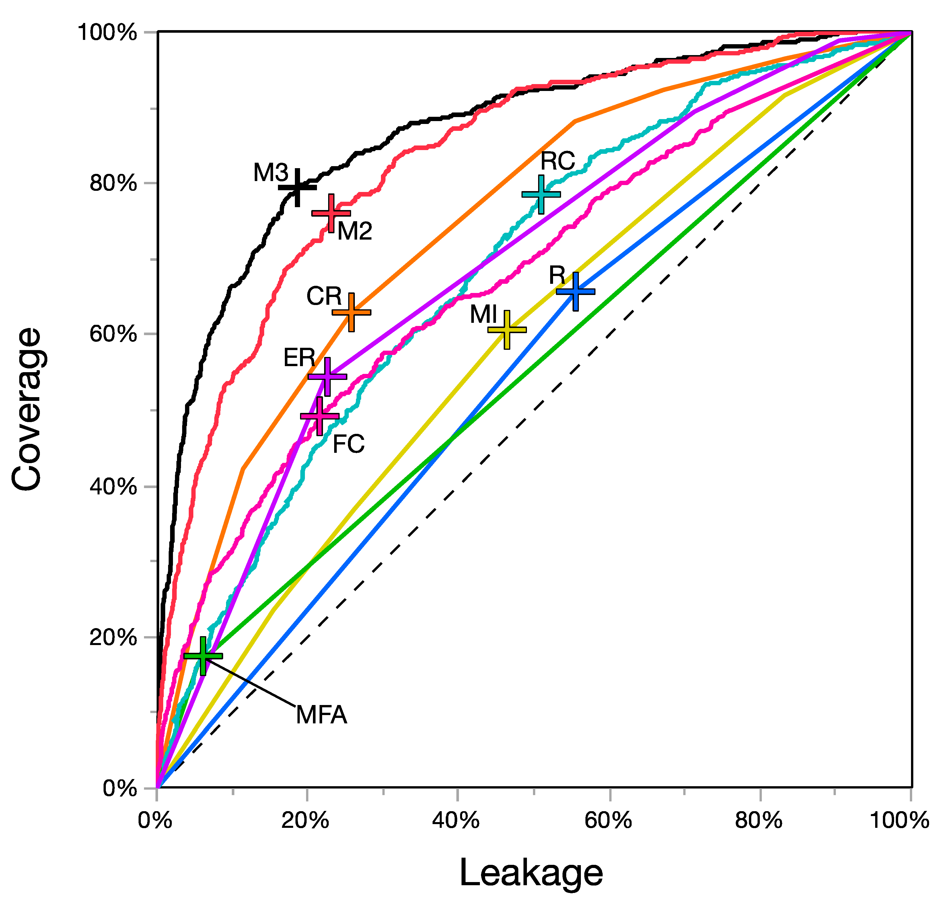
3.2.1. Targeting Coverage and Leakage

Each priority criterion’s main effects (unadjusted) on AEM distribution in Model 1 were statistically significant (α = 0.05) (

Table 2. Fit statistics for simple (Model 1) and multiple (Models 2 and 3) logistic regression models.

	AUC	R2 (M)	R2 (N)	LRT	p-Value	AICc	BIC
Model 3 (multiple)	0.87	0.33	0.45	864	<0.0001	1808	1964
Model 2 (multiple)	0.83	0.26	0.37	673	<0.0001	1982	2092
Model 1 (simple)
Climate region (CR)	0.75	0.14	0.21	359	<0.0001	2274	2321
Erosion risk (ER)	0.69	0.09	0.14	230	<0.0001	2395	2418
Rainfed cropland (RC)	0.69	0.03	0.05	83	<0.0001	2538	2550
Failed cropland (FC)	0.68	0.06	0.10	160	<0.0001	2461	2473
Marginalization (MI)	0.59	0.02	0.03	47	<0.0001	2580	2609
Mean farm area (MFA)	0.56	0.02	0.04	61	<0.0001	2560	2572
Rural classification (R)	0.55	0.01	0.01	18	<0.0001	2603	2614

). Climate region and erosion risk had larger whole effects than other criteria, the highest likelihood ratio tests (LRTs), highest pseudo-R-squared (M and N), and lowest information criteria scores (AICc and BIC). Climate region and erosion risk also produced the highest singular AUC values, correctly explaining AEM distribution 75 and 69 percent of the time.

Overall, Models 2 and 3 explained AEM distribution about 83 and 87 percent of the time, respectively, which indicates good to excellent discriminatory capacity [77]. The controls imposed on Model 3 improved the success rate from Model 2 by about three percent (AUC = 0.866–0.834). Pseudo-r-squared measures were higher in Model 3 (McFadden = 0.33, Nagelkerke = 0.45) than in Model 2 (McFadden = 0.26, Nagelkerke = 0.37); likelihood ratio tests also were higher (Model 3 = 864, Model 2 = 673); and Model 3 had lower AICc (Model 3 = 1808, Model 2 = 1964) and BIC (Model 3 = 1982, Model 2 = 2092) scores (Table 2).

The probability threshold cutoff points for Models 2 and 3 as determined by the Youden Index were 0.201 and 0.198, respectively. At these optimization points, Models 2 and 3 correctly explained AEM(Y) about 77 and 80 percent of the time, respectively (Figure 1). The under-coverage rates of Model 2 and Model 3 were 23 and 20 percent, respectively, while over-coverage rates were 24 and 19 percent, respectively (

Table 3. Coverage and leakage rates for Models 2 and 3. Bold values refer to coverage rates, bold italicized values to over-coverage rates, and italicized values to under-coverage rates.

			Observed AEM
	Model		No	Yes
Predicted	2	No	75.72%	23.01%
AEM		Yes	24.28%	76.99%
	3	No	81.14%	20.29%
		Yes	18.86%	79.71%

).

The overall coverage rate of Model 3 was 79–80 percent, and the leakage rate was 19–20 percent. The targeting errors of Model 3 showed AEM were misallocated to non-priority municipalities 19 percent of the time (inclusion error), while priority municipalities were excluded from receiving AEM 20 percent of the time (exclusion error).

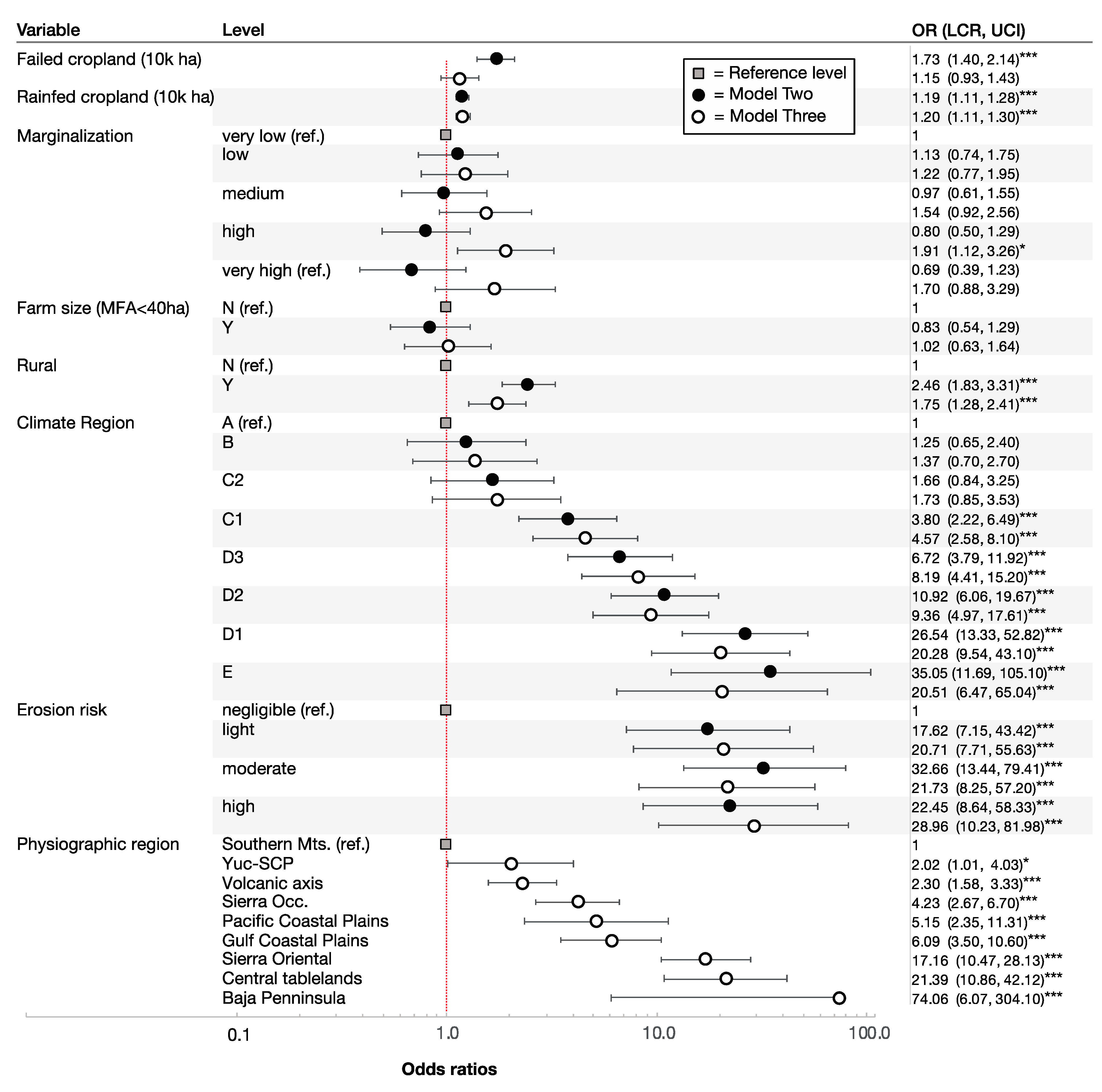
3.2.2. Positive Odds of Receiving AEM per Priority Criterion

Within these overall measures of targeting effectiveness, the roles of each targeting criterion in determining AEM(Y) varied widely. In other words, the coverage–leakage rates above were determined only after the models assigned very different effects to each of the explanatory variables.

Failed cropland was a strong determinant of AEM(Y) in Model 2 but a weak determinant in Model 3. The odds of AEM(Y) increased 73 percent with every one-unit (10,000 ha) increase in failed cropland in Model 2 but fell to a statistically insignificant 15 percent once adjusted for SAC and physiographic region (Model 3). Rainfed cropland was a statistically significant determinant in both models. The odds of AEM(Y) increased by 19 and 20 percent with every one-unit increase in rainfed cropland in Models 2 and 3, respectively (Figure 2).

Marginalization level was negatively associated with AEM(Y) in Model 2. Compared to municipalities with very low marginalization, those with medium, high, and very high were 3, 20, and 31 percent less likely to receive AEM, respectively, although these effects were not statistically significant. The association reversed after the adjustments of Model 3, where the odds of AEM(Y) in municipalities with low, medium, high, and very high marginality were 22, 54, 91, and 70 percent higher, respectively. However, even in Model 3, only the high-marginality classification effects were statistically significant.

Mean farm area of municipalities had little effect on AEM distribution. Municipalities with mean farm areas less than 40 ha (target classification) were 17 percent less likely to receive AEM in Model 2. In Model 3 the effect was negligible and statistically insignificant. Contrasting with this, the rural municipality classification was a significant determinant of AEM(Y). Rural municipalities were 146 percent more likely to receive AEM than non-rural municipalities in Model 2 and 75 percent more likely in Model 3.

Climate region was a strong determinant of AEM distribution. In Model 2, the odds of AEM(Y) in the most arid regions (E, D1, and D2) were 35, 27, and 11 times higher, respectively, than in the perhumid region (A). These odds fell to 21, 20, and 9 times higher in Model 3. In humid regions the adjustment effects of Model 3 were smaller. Overall, the positive relationship between aridity and the odds of AEM(Y) was strong, statistically significant, and relatively consistent between Models 2 and 3.

Erosion risk also was a strong determinant of AEM distribution. Compared to municipalities with the lowest erosion risk (negligible), the odds of AEM(Y) in municipalities with low, moderate, and high risk were 18, 33, and 23 times higher, respectively, in Model 2. The positive (ordered) association between erosion risk and the odds of AEM(Y) was clearer in Model 3. Here, the odds of AEM(Y) in municipalities with low, moderate, and high risk increased sequentially at 21, 22, and 29 times higher, respectively.

Physiographic region, like climate and erosion risk, was a strong and statistically significant determinant of AEM distribution. Unlike the other variables, however, the different physiographic regions (PRs) did not reflect a logical value ordering based on program criteria. However, for illustrative purposes we ordered the PR levels in a general north-trending sequence. This showed that municipalities in the northern regions of the Eastern Mountains, Central Tablelands, and Baja Peninsula were about 17, 21, and 74 times more likely, respectively, to receive AEM than municipalities in the southern most region (Southern Mountains). Inclusion of PR satisfied model assumptions and controlled the effects of SAC, and moderately attenuated the effects of climate regions and erosion risk on AEM distribution. However, the largest attenuating effects of PR were on the relationship between marginality and AEM distribution.

Overall, the effects of climate zone, erosion risk, and physiographic region were the strongest determinants of AEM distribution in both models. The partial effects of climate region showed strong positive association between aridity and the odds of receiving AEM. The other priority criteria were less significant, despite being described in program rules as important determinants of AEM distribution (Figure 2).

4. Discussion

Our logistic models explained the distribution of agri-environmental measures in one of Mexico’s largest support programs about 83 to 87 percent of the time. The targeting strategy had coverage and leakage rates of about 80 and 20 percent, respectively. These findings suggest a relatively effective targeting strategy [41,77,79]. However, closer examination reveals significant differences in the whole and partial effects of the seven priority criteria on AEM distribution. Climate region and erosion risk indicators were far better determinants of AEM distribution than were a municipality’s mean farmland size, rainfed land area, failed cropland area, or marginalization level.

4.1. AEM Targeting Favors Arid Regions at Risk of Soil Erosion

The observed distribution of AEM reflects Mexico’s strong policy emphasis on addressing hydroclimatic vulnerability and the effects of desertification on agriculture [80]. Municipalities in arid and semi-arid regions at high risk of soil erosion were about 20 times more likely to receive AEM than wetter municipalities with little erosion risk. About 65 percent of Mexican territory is dry (hyper-arid, arid, semi-arid, and sub-humid) [81], and about 60 percent of agriculture is rainfed and thus susceptible to climatic variability [82]. This vulnerability of rainfed agriculture to drought has played a major role in institutional responses to cropland failure over the last several decades [83,84], which come in the form of emergency relief, subsidies, and agri-environmental support measures [48,49,50]. Unlike the differences we found among climate regions, we found no significant differences among the low, medium, and high erosion risk classifications in the likelihood of receiving AEM (Model 3). This suggests that the program did not target AEM based on erosion risk distinctions to the same degree it did based on climate region distinctions. In general, aridity was a stronger determinant than erosion risk.

While the PIASRE program successfully targeted AEM to dry regions with some erosion risk, the conceptual basis for prioritizing these factors over regions with high levels of failed cropland is unclear. Furthermore, the lack of specificity in program rules in how to define and constrain the climate region, erosion risk, and failed cropland criteria makes assessing these relationships problematic. Ultimately, this lack of clarity serves as a major impediment to any meaningful ex-post assessment of policy effectiveness beyond the immediate, indicator-based targeting strategy.

4.2. AEM Targeting Neglects Marginalized Smallholder Farms

A 2009 report by the World Bank characterized the PIASRE program as specifically targeted to the rural poor, although the reasoning behind the characterization is unclear [50,85]. Our assessment found weak evidence that the program prioritized poor rural areas for AEM distribution. Instead, we found a negative relationship between marginalization and the likelihood of receiving AEM in Model 2, and only a slightly higher likelihood of receiving AEM among municipalities with high levels of marginalization in Model 3.

The discrepancy between the above characterization and our findings has at least two possible explanations: definitional ambiguity and characterization based on the targeting rules, rather than the actual distribution of AEM. First, there are many different methods for defining and measuring poverty in Mexico, and as the report notes, methods often vary across policies [50]. In the current case, PIASRE program rules specify using marginalization level as the priority indicator, marginalization being a common metric of multidimensional poverty in Mexico [58,59,60]. Therefore, definitional ambiguity does not explain the different characterizations.

A more likely explanation is that the characterization was based on the program’s targeting rules [52,53,57] rather than on observed coverages. The report acknowledges that leakages typically prevent some targeted support from reaching poorer regions but does not specify the nature or scale of leakages in the PIASRE program [50]. Our study confirms that the program was targeted to the rural poor, but only at the level of program design. The observed distribution of AEM was minimally aligned with the poverty targeting priorities in program rules. That is, the targeting strategy effectively failed to prioritize Mexico’s poorest regions, resulting instead in targeting under-coverages and more general policy leakages. Other studies confirm significant leakages in Mexican agricultural [49] and development policy [79], though these leakages are seldom quantified. This is due, in part, to transparency issues and the lack of available program data [86].

The leakages identified in this study reflect a broader institutional neglect of smallholder agriculture in Mexico. Despite rhetoric, policies have long failed to provide support to small farms, tending instead to distribute support to larger and wealthier farms [87,88]. In Mexico, close associations exist between smallholder agriculture, rural poverty, lack of access to irrigation, degraded or marginal farmland, and agricultural vulnerability more generally [89,90,91]. Commonly classified as having fewer than five hectares, smallholder farms in Mexico comprise about 72 percent of all farms but hold only about 18 percent of all cultivated land [49]. PIASRE program rules specified that farms smaller than 40 ha should be prioritized for AEM—a range that would include very small, small, medium, and many large farms [63]. Yet we found no statistically significant relationship between mean farm area and AEM distribution—municipalities with mean farm areas smaller than 40 ha were no more likely to receive AEM than municipalities with areas greater than 40 ha. Although Mexican agricultural policy has expanded to address a broader range of socioeconomic and environmental concerns, our study highlights the persistent neglect of its poorest farming regions. This has occurred despite enhanced legal requirements and some outward improvements in transparency over the last several decades [49,86].

4.3. Targeting Gaps in Agri-Environmental Policy Implementation

Gaps between stated program rules and the observed distribution of support are largely attributable to the absence of value ordering among the targeting criteria. In place of an explicit value order, our study reveals the implicit ordering of priorities based on ex-post assessment of the observed distribution. Value ordering of priority criteria is key to policy effectiveness when multiple objectives are involved in targeting [4,19]. Conflicts can emerge among objectives, e.g., optimizing equity verses efficiency [92,93], which may require tradeoffs and careful analyses of interaction or spillover effects [6]. These effects can be highly variable in space and time. Recognition of this variability has driven calls for indicator-based approaches to targeting assessment and the selection of priority criteria [2,19,94]. In the case of the PIASRE program, similar indicator-based approaches to assessment could be used to provide the framework for a more empirically grounded value ordering of criteria.

It is beyond the scope of this study to explore whether the PIASRE program’s targeting strategy would have achieved beneficial results if properly implemented. A two-year experimental case study found that the program produced mixed benefits [95]. Support measures were targeted to address a specific soil and water conservation objective, although the incentive structure produced only short-term conservation benefits. In the medium to longer terms, support measure actions actually resulted in landscape degradation. In addition, the empirical results needed to make this assessment required a level of intensive and sustained field monitoring that is seldom practical over larger spatial scales and timeframes.

Such site-level experimental approaches constitute the greatest share of ex-post assessment of the environmental effects of AEM. The spatiotemporal limitations associated with these approaches often result in a general lack of understanding of targeting effects on larger-scale processes [9]. Additional challenges to assessing larger-scale processes include the high costs of monitoring and measurement and the lack of linearity and immediacy of AEM effects [96]. Indeed, misalignment between institutional and ecosystem timeframes is a complicating scale effect that is often encountered when working at the intersection of social and ecological systems [97]. The design and evaluation of multi-objective agri-environmental policy requires similarly synthetic approaches to socioenvironmental systems science [98]. As such, improved integration of agri-environmental policy approaches remains a central challenge to targeting design, implementation, and evaluation [92].

We cannot say with certainty why smallholders in poor regions prone to cropland failure failed to receive a greater share of support, as required by program rules. The program’s over-coverage of arid and semi-arid regions may reflect legitimate concerns or policy changes that remain unexplained. Furthermore, we recognize that budgetary factors may have played a role in the targeting strategy, though we were unable to assess this as these data were unavailable. We also did not investigate the willingness or unwillingness of farmers to participate as a determinant of AEM distribution though we recognize its potential relevance [7,8]. Previous research shows that support programs involving little actual change in farming practices often generate higher farmer participation [12]. One study shows the land management practices supported by the PIASRE program were already in widespread use in marginalized smallholder regions [99], which would suggest a higher willingness to participate. Further research into the specific drivers of the targeting leakages identified in this study is needed. The methods developed in this study also could be applied to examine targeting strategies in rural humanitarian and development contexts, helping policymakers better target support to reduce poverty and vulnerability, conflict, and famine [37,38].

The push for greater policy focus on results-based targeting of agri-environmental measures is growing in Europe [8,100,101]. In Mexico, results-based targeting is also discussed, but in the context of payments for hydrological services and biodiversity conservation [102,103]. Mexico has one of the largest payments for ecosystem services programs in the world, which the country manages through the Ministry of the Environment and Natural Resources (SEMARNAT) and the National Forestry Commission (CONAFOR) [104,105]. Although separate ministries, some integration of these efforts with SADER policy could help generate the results- and indicator-based assessments of AEM that are needed in Mexico [88,94]. In turn, findings from these combined efforts could better inform the selection and value ordering of priority criteria—a factor critical not only to the design of targeting strategies but also to their effective implementation.

5. Conclusions

We used logistic models, ROC curves, and odds ratios to assess the targeting coverages and leakages of Mexico’s PIASRE program, which distributed agricultural support measures to farms across the country based on seven priority criteria. Our results show that despite coverage and leakage rates of 80 and 20 percent, respectively, large differences exist in priority criteria effects on AEM distribution. While the program favored arid and semi-arid regions at risk of soil erosion, it neglected poor smallholder farming regions with high levels of cropland failure. These targeting gaps reveal that despite new legislation and some outward improvements in transparency, actual policy support for smallholder agriculture remains inadequate. Better structural alignment between the design and implementation of targeting strategies is needed. This alignment is a critical though often overlooked determinant of targeting precision and overall policy effectiveness.

References

1. Song, B.; Robinson, G.M. Multifunctional Agriculture: Policies and Implementation in China. Geogr. Compass 2020, 14, e12538. [Google Scholar] [CrossRef]
2. Longo, M.; Dal Ferro, N.; Lazzaro, B.; Morari, F. Trade-Offs among Ecosystem Services Advance the Case for Improved Spatial Targeting of Agri-Environmental Measures. J. Environ. Manag. 2021, 285, 112131. [Google Scholar] [CrossRef] [PubMed]
3. Pannell, D.J.; Roberts, A.M.; Park, G.; Alexander, J.; Curatolo, A.; Marsh, S.P. Integrated Assessment of Public Investment in Land-Use Change to Protect Environmental Assets in Australia. Land Use Policy 2012, 29, 377–387. [Google Scholar] [CrossRef]
4. Uthes, S.; Matzdorf, B.; Müller, K.; Kaechele, H. Spatial Targeting of Agri-Environmental Measures: Cost-Effectiveness and Distributional Consequences. Environ. Manag. 2010, 46, 494–509. [Google Scholar] [CrossRef]
5. Mettepenningen, E.; Beckmann, V.; Eggers, J. Public Transaction Costs of Agri-Environmental Schemes and Their Determinants—Analysing Stakeholders’ Involvement and Perceptions. Ecol. Econ. 2011, 70, 641–650. [Google Scholar] [CrossRef]
6. Huber, R.; Rebecca, S.; François, M.; Hanna, B.S.; Dirk, S.; Robert, F. Interaction Effects of Targeted Agri-Environmental Payments on Non-Marketed Goods and Services under Climate Change in a Mountain Region. Land Use Policy 2017, 66, 49–60. [Google Scholar] [CrossRef]
7. Del Rossi, G.; Hecht, J.S.; Zia, A. A Mixed-Methods Analysis for Improving Farmer Participation in Agri-Environmental Payments for Ecosystem Services in Vermont, USA. Ecosyst. Serv. 2021, 47, 101223. [Google Scholar] [CrossRef]
8. Niskanen, O.; Tienhaara, A.; Haltia, E.; Pouta, E. Farmers’ Heterogeneous Preferences towards Results-Based Environmental Policies. Land Use Policy 2021, 102, 105227. [Google Scholar] [CrossRef]
9. Bertoni, D.; Curzi, D.; Aletti, G.; Olper, A. Estimating the Effects of Agri-Environmental Measures Using Difference-in-Difference Coarsened Exact Matching. Food Policy 2020, 90, 101790. [Google Scholar] [CrossRef]
10. Šumrada, T.; Erjavec, E. Designs and characteristics of agri-environmental measures. Acta Agric. Slov. 2020, 116, 157–178. [Google Scholar] [CrossRef]
11. Galler, C.; von Haaren, C.; Albert, C. Optimizing Environmental Measures for Landscape Multifunctionality: Effectiveness, Efficiency and Recommendations for Agri-Environmental Programs. J. Environ. Manag. 2015, 151, 243–257. [Google Scholar] [CrossRef]
12. Burton, R.J.F.; Schwarz, G. Result-Oriented Agri-Environmental Schemes in Europe and Their Potential for Promoting Behavioural Change. Land Use Policy 2013, 30, 628–641. [Google Scholar] [CrossRef] [Green Version]
13. Pakeman, R.J.; McKeen, M. Within Country Targeting of Agri-Environment Funding: A Test of Different Methods. Glob. Ecol. Conserv. 2019, 17, e00574. [Google Scholar] [CrossRef]
14. Mauchline, A.L.; Mortimer, S.R.; Park, J.R.; Finn, J.A.; Haysom, K.; Westbury, D.B.; Purvis, G.; Louwagie, G.; Northey, G.; Primdahl, J.; et al. Environmental Evaluation of Agri-Environment Schemes Using Participatory Approaches: Experiences of Testing the Agri-Environmental Footprint Index. Land Use Policy 2012, 29, 317–328. [Google Scholar] [CrossRef]
15. Whittaker, G.; Färe, R.; Grosskopf, S.; Barnhart, B.; Bostian, M.; Mueller-Warrant, G.; Griffith, S. Spatial Targeting of Agri-Environmental Policy Using Bilevel Evolutionary Optimization. Omega 2017, 66, 15–27. [Google Scholar] [CrossRef]
16. Kubacka, M.; Bródka, S.; Macias, A. Selecting Agri-Environmental Indicators for Monitoring and Assessment of Environmental Management in the Example of Landscape Parks in Poland. Ecol. Indic. 2016, 71, 377–387. [Google Scholar] [CrossRef]
17. Matzdorf, B.; Kaiser, T.; Rohner, M.-S. Developing Biodiversity Indicator to Design Efficient Agri-Environmental Schemes for Extensively Used Grassland. Ecol. Indic. 2008, 8, 256–269. [Google Scholar] [CrossRef]
18. Slabe-Erker, R.; Bartolj, T.; Ogorevc, M.; Kavaš, D.; Koman, K. The Impacts of Agricultural Payments on Groundwater Quality: Spatial Analysis on the Case of Slovenia. Ecol. Indic. 2017, 73, 338–344. [Google Scholar] [CrossRef]
19. Raggi, M.; Viaggi, D.; Bartolini, F.; Furlan, A. The Role of Policy Priorities and Targeting in the Spatial Location of Participation in Agri-Environmental Schemes in Emilia-Romagna (Italy). Land Use Policy 2015, 47, 78–89. [Google Scholar] [CrossRef]
20. Bartolini, F.; Brunori, G.; Fastelli, L.; Rovai, M. Understanding the Participation in Agri-Environmental Schemes: Evidence from Tuscany Region; European Regional Science Association (ERSA): Louvain-la-Neuve, Belgium, 2013. [Google Scholar]
21. Batáry, P.; Báldi, A.; Kleijn, D.; Tscharntke, T. Landscape-Moderated Biodiversity Effects of Agri-Environmental Management: A Meta-Analysis. Proc. R. Soc. B 2011, 278, 1894–1902. [Google Scholar] [CrossRef]
22. Rodríguez-Ortega, T.; Olaizola, A.M.; Bernués, A. A Novel Management-Based System of Payments for Ecosystem Services for Targeted Agri-Environmental Policy. Ecosyst. Serv. 2018, 34, 74–84. [Google Scholar] [CrossRef]
23. Bredemeier, B.; von Haaren, C.; Rüter, S.; Reich, M.; Meise, T. Evaluating the Nature Conservation Value of Field Habitats: A Model Approach for Targeting Agri-Environmental Measures and Projecting Their Effects. Ecol. Model. 2015, 295, 113–122. [Google Scholar] [CrossRef]
24. Mueller, N.D.; Gerber, J.S.; Johnston, M.; Ray, D.K.; Ramankutty, N.; Foley, J.A. Closing Yield Gaps through Nutrient and Water Management. Nature 2012, 490, 254–257. [Google Scholar] [CrossRef] [PubMed]
25. Kleijn, D.; Sutherland, W.J. How Effective Are European Agri-Environment Schemes in Conserving and Promoting Biodiversity? J. Appl. Ecol. 2003, 40, 947–969. [Google Scholar] [CrossRef]
26. Heller, M.C.; Walchale, A.; Heard, B.R.; Hoey, L.; Khoury, C.K.; De Haan, S.; Burra, D.D.; Duong, T.T.; Osiemo, J.; Trinh, T.H.; et al. Environmental Analyses to Inform Transitions to Sustainable Diets in Developing Countries: Case Studies for Vietnam and Kenya. Int. J. Life Cycle Assess. 2020, 25, 1183–1196. [Google Scholar] [CrossRef]
27. Nori-Sarma, A.; Gurung, A.; Azhar, G.S.; Rajiva, A.; Mavalankar, D.; Sheffield, P.; Bell, M.L. Opportunities and Challenges in Public Health Data Collection in Southern Asia: Examples from Western India and Kathmandu Valley, Nepal. Sustainability 2017, 9, 1106. [Google Scholar] [CrossRef] [Green Version]
28. Ponette-González, A.G.; Brauman, K.A.; Marín-Spiotta, E.; Farley, K.A.; Weathers, K.C.; Young, K.R.; Curran, L.M. Managing Water Services in Tropical Regions: From Land Cover Proxies to Hydrologic Fluxes. Ambio 2015, 44, 367–375. [Google Scholar] [CrossRef] [Green Version]
29. Dany, V.; Bowen, K.J.; Miller, F. Assessing the Institutional Capacity to Adapt to Climate Change: A Case Study in the Cambodian Health and Water Sectors. Clim. Policy 2015, 15, 388–409. [Google Scholar] [CrossRef] [Green Version]
30. Bibi, S.; Duclos, J.-Y. Equity and Policy Effectiveness with Imperfect Targeting. J. Dev. Econ. 2007, 83, 109–140. [Google Scholar] [CrossRef] [Green Version]
31. Seleka, T.B.; Lekobane, K.R. Targeting Effectiveness of Social Transfer Programs in Botswana: Means-Tested versus Categorical and Self-Selected Instruments. Soc. Dev. Issues 2020, 42, 20. [Google Scholar] [CrossRef]
32. Bah, A.; Bazzi, S.; Sumarto, S.; Tobias, J. Finding the Poor vs. Measuring Their Poverty: Exploring the Drivers of Targeting Effectiveness in Indonesia. World Bank Econ. Rev. 2019, 33, 573–597. [Google Scholar] [CrossRef] [Green Version]
33. Wodon, Q.T. Targeting the Poor Using ROC Curves. World Dev. 1997, 25, 2083–2092. [Google Scholar] [CrossRef]
34. Chaaban, J.; Ghattas, H.; Irani, A.; Thomas, A. Targeting Mechanisms for Cash Transfers Using Regional Aggregates. Food Sec. 2018, 10, 457–472. [Google Scholar] [CrossRef] [Green Version]
35. Masud-All-Kamal, M.; Saha, C.K. Targeting Social Policy and Poverty Reduction: The Case of Social Safety Nets in Bangladesh. Poverty Public Policy 2014, 6, 195–211. [Google Scholar] [CrossRef]
36. Houssou, N.; Zeller, M. To Target or Not to Target? The Costs, Benefits, and Impacts of Indicator-Based Targeting. Food Policy 2011, 36, 627–637. [Google Scholar] [CrossRef]
37. Agurto, M.; Calvo, C.H.; Carpio, M. Targeting When Poverty Is Multidimensional; Partnersh. Econ. Policy Work.: Rochester, NY, USA, 2020; p. 21. [Google Scholar]
38. van de Walle, D. Targeting Revisited. World Bank Res. Obs. 1998, 13, 231–248. [Google Scholar] [CrossRef]
39. Guo, Y.; Zheng, H.; Wu, T.; Wu, J.; Robinson, B.E. A Review of Spatial Targeting Methods of Payment for Ecosystem Services. Geogr. Sustain. 2020, 1, 132–140. [Google Scholar] [CrossRef]
40. Ponette-González, A.G.; Fry, M. Enduring Footprint of Historical Land Tenure on Modern Land Cover in Eastern Mexico: Implications for Environmental Services Programmes. Area 2014, 46, 398–409. [Google Scholar] [CrossRef]
41. Verme, P.; Gigliarano, C. Optimal Targeting under Budget Constraints in a Humanitarian Context. World Dev. 2019, 119, 224–233. [Google Scholar] [CrossRef]
42. Bigman, D.; Fofack, H. Geographical Targeting for Poverty Alleviation: An Introduction to the Special Issue. World Bank Econ. Rev. 2000, 14, 129–145. [Google Scholar] [CrossRef]
43. Zhu, L.; Zhang, C.; Cai, Y. Varieties of Agri-Environmental Schemes in China: A Quantitative Assessment. Land Use Policy 2018, 71, 505–517. [Google Scholar] [CrossRef]
44. Orozco-Ramírez, Q.; Astier, M.; Barrasa, S. Agricultural Land Use Change after NAFTA in Central West Mexico. Land 2017, 6, 66. [Google Scholar] [CrossRef] [Green Version]
45. Wu, F.; Qushim, B.; Calle, M.; Guan, Z. Government Support in Mexican Agriculture. Choices 2018, 33, 1–11. [Google Scholar]
46. Ríos-Carmenado, I.D.L.; Díaz-Puente, J.M.; Cadena-Iñiguez, J. La iniciativa LEADER como modelo de desarrollo rural: Aplicación a algunos territorios de México. Agrociencia 2011, 45, 609–624. [Google Scholar]
47. DOF. Ley de Desarrollo Rural Sostenible. Secretaría de Agricultura, Ganadería, Pesca y Alimenta (SAGARPA); Diario Oficial de la Federación (DOF): Mexico City, Mexico, 2001.
48. Zamora, A.M.; Velázquez, M.A.J.; Cué, J.L.G. Rural Agricultural Development and Extension in Mexico: Analysis of Public and Private Extension Agents. J. Agric. Ext. Rural Dev. 2017, 9, 283–291. [Google Scholar] [CrossRef] [Green Version]
49. UNCTAD. Mexico’s Agriculture Development: Perspective and Outlook; United Nations Conference on Trade and Development: Geneva, NY, USA, 2014; p. 175. [Google Scholar]
50. World Bank. Mexico: Agriculture and Rural Development Public Expenditure Review. Agriculture and Rural Development Unit; The World Bank: Washington, DC, USA, 2009; p. 127. [Google Scholar]
51. Gómez Oliver, L.G.; Tacuba Santos, A. La política de desarrollo rural en México. ¿Existe correspondencia entre lo formal y lo real? The rural development policy in Mexico. Is there correspondence between the formal and the real? Econ. unam 2017, 14. [Google Scholar] [CrossRef]
52. FAO-SAGARPA. Informe de Evaluación de Consistencia y Resultados 2007: Programa Integral de Agricultural Sostenible y Reconversión Productiva En Zonas de Siniestralidad Recurrente (PIASRE); SAGARPA-CONZA: Mexico City, Mexico, 2008; p. 155.
53. SAGARPA. Reglas de Operación del Programa Integral de Agricultura Sostenible y Reconversión Productiva en Zonas de Siniestralidad Recurrente (PIASRE); Secretaría de Agricultural y Ganadería, Diario Oficial de la Federación: Mexico City, Mexico, 2003.
54. PIASRE-SAGARPA. Padrónes de beneficiarios (31 estados y el Distrito Federal); PIASRE-SAGARPA: Mexico City, Mexico, 2008.
55. CAP. Censo Agrícola, Ganadero y Forestal 2007 (Censo Agropecuario); Instituto Nacional de Estadística y Geografía (INEGI): Mexico City, Mexico, 2008.
56. SIAP. Estadística de la Producción Agrícola (2002–2006); Servicio de Información Agroalimentaría y Pesquera; Secretaría de Agricultura y Desarrollo Rural: Mexico City, Mexico, 2020.
57. SAGARPA. Informe de Ejecución Del Programa Nacional de Población: 2001–2006; SAGARPA: Mexico City, Mexico, 2006.
58. Pinzón Florez, C.E.; Reveiz, L.; Idrovo, A.J.; Reyes Morales, H. Gasto en salud, la desigualdad en el ingreso y el índice de marginación en el sistema de salud de México. Rev. Panam. Salud Publica 2014, 35, 1–7. [Google Scholar] [PubMed]
59. Cortés, F.; Vargas, D. Marginación En México a Través Del Tiempo: A Propósito Del Índice de Conapo. Estud. Sociol. 2011, 29, 361–387. [Google Scholar]
60. García Chong, N.R.; Salvatierra Izaba, B.; Trujillo Olivera, L.E.; Zúñiga Cabrera, M. Mortalidad infantil, pobreza y marginación en indígenas de los altos de Chiapas, México. Ra Ximhai 2010, 115–130. [Google Scholar] [CrossRef]
61. CONAPO. Indice De Marginación Por Município 2005; Comisión Nacional de Población: Mexico City, Mexico, 2020.
62. INAFED Sistema Nacional De Información Municipal (SNIM) Base De Datos 2005; Instituto Nacional para el Federalismo y el Desarrollo Municipal: Mexico City, Mexico, 2020.
63. LaFevor, M.C.; Magliocca, N.R. Farmland Size, Chemical Fertilizers, and Irrigation Management Effects on Maize and Wheat Yield in Mexico. J. Land Use Sci. 2020, 15, 532–546. [Google Scholar] [CrossRef]
64. Samberg, L.H.; Gerber, J.S.; Ramankutty, N.; Herrero, M.; West, P.C. Subnational Distribution of Average Farm Size and Smallholder Contributions to Global Food Production. Environ. Res. Lett. 2016, 11, 124010. [Google Scholar] [CrossRef]
65. CONAZA; UACH. Escenarios Climatológicos De La República Mexicana Ante El Cambio Climático; Universidad Autónoma Chapingo (CONAZA), Dirección de Vinculación y: Mexico City, Mexico, 2003; ISBN 968-884-941-3. [Google Scholar]
66. SEMARNAT. CP Evaluación De La Degradación Del Suelo Causada Por El Hombre En La República Mexicana, Escala 1:250,000. Memoria Nacional; SEMARNAT: Mexico City, Mexico, 2003.
67. Cullen, P.; Ryan, M.; O’Donoghue, C.; Hynes, S.; hUallacháin, D.Ó.; Sheridan, H. Impact of Farmer Self-Identity and Attitudes on Participation in Agri-Environment Schemes. Land Use Policy 2020, 95, 104660. [Google Scholar] [CrossRef]
68. van der Sluis, T.; Pedroli, B.; Kristensen, S.B.P.; Lavinia Cosor, G.; Pavlis, E. Changing Land Use Intensity in Europe—Recent Processes in Selected Case Studies. Land Use Policy 2016, 57, 777–785. [Google Scholar] [CrossRef]
69. Unay Gailhard, İ.; Bojnec, Š. Farm Size and Participation in Agri-Environmental Measures: Farm-Level Evidence from Slovenia. Land Use Policy 2015, 46, 273–282. [Google Scholar] [CrossRef]
70. Bo, Y.-C.; Song, C.; Wang, J.-F.; Li, X.-W. Using an Autologistic Regression Model to Identify Spatial Risk Factors and Spatial Risk Patterns of Hand, Foot and Mouth Disease (HFMD) in Mainland China. BMC Public Health 2014, 14, 358. [Google Scholar] [CrossRef] [Green Version]
71. Crase, B.; Liedloff, A.C.; Wintle, B.A. A New Method for Dealing with Residual Spatial Autocorrelation in Species Distribution Models. Ecography 2012, 35, 879–888. [Google Scholar] [CrossRef]
72. Huang, Q.-H.; Cai, Y.-L.; Peng, J. Modeling the Spatial Pattern of Farmland Using GIS and Multiple Logistic Regression: A Case Study of Maotiao River Basin, Guizhou Province, China. Environ. Model. Assess. 2007, 12, 55–61. [Google Scholar] [CrossRef]
73. Hu, Z.; Lo, C.P. Modeling Urban Growth in Atlanta Using Logistic Regression. Comput. Environ. Urban Syst. 2007, 31, 667–688. [Google Scholar] [CrossRef]
74. Wang, W.-C.; Chang, Y.-J.; Wang, H.-C. An Application of the Spatial Autocorrelation Method on the Change of Real Estate Prices in Taitung City. ISPRS Int. J. Geo-Inf. 2019, 8, 249. [Google Scholar] [CrossRef] [Green Version]
75. INEGI, (Instituto Nacional de Estadística y Geografía. Conjunto De Datos Vectoriales Escala 1:1000000, Provincias Fisiográficas; Instituto Nacional de Geografía y Estadística: Mexico City, Mexico, 2020.
76. Baulch, B. Poverty Monitoring and Targeting Using ROC Curves: Examples from Vietnam; Institute of Development Studies: Brighton, UK, 2002; p. 27. [Google Scholar]
77. Mandrekar, J.N. Receiver Operating Characteristic Curve in Diagnostic Test Assessment. J. Thorac. Oncol. 2010, 5, 1315–1316. [Google Scholar] [CrossRef] [PubMed] [Green Version]
78. Goksuluk, D.; Korkmaz, S.; Zararsiz, G.; Karaagaoglu, A.E. EasyROC: An Interactive Web-Tool for ROC Curve Analysis Using R Language Environment. R J. 2016, 8, 19. [Google Scholar] [CrossRef] [Green Version]
79. Skoufias, E.; Davis, B.; de la Vega, S. Targeting the Poor in Mexico: An Evaluation of the Selection of Households into PROGRESA. World Dev. 2001, 29, 1769–1784. [Google Scholar] [CrossRef]
80. Sámano-Romero, G.; Mautner, M.; Chávez-Mejía, A.; Jiménez-Cisneros, B. Assessing Marginalized Communities in Mexico for Implementation of Rainwater Catchment Systems. Water 2016, 8, 140. [Google Scholar] [CrossRef] [Green Version]
81. Verbist, K.; Santibañez, F.; Gabrieles, D.; Soto, G. Atlas De Zonas Áridas De América Latina y el Caribe; Proyecto realizado en el marco de UNESCO-PHI y del Gobierno de Flandes, Departamento de Ciencias e Innovaciones; UNESCO: Montevideo, Uruguay, 2010; p. 55. [Google Scholar]
82. Conde, C.; Ferrer, R.; Orozco, S. Climate Change and Climate Variability Impacts on Rainfed Agricultural Activities and Possible Adaptation Measures. A Mexican Case Study. Atmósfera 2006, 19, 181–194. [Google Scholar]
83. Liverman, D.M. Vulnerability and Adaptation to Drought in Mexico. Nat. Resour. J. 1999, 39, 99. [Google Scholar]
84. Liverman, D.M. Drought Impacts in Mexico: Climate, Agriculture, Technology, and Land Tenure in Sonora and Puebla. Ann. Assoc. Am. Geogr. 1990, 80, 49–72. [Google Scholar] [CrossRef]
85. Oliver, L.; Santillanes, S. Cuantificación y Clasificación Del Gasto Público Rural En México: Informe Presentado al Banco Mundial; World Bank: Washington, DC, USA, 2008. [Google Scholar]
86. Fox, J.; Haight, L. Subsidizing Inequality: Mexican Corn Policy Since NAFTA|Wilson Center; Woodrow Wilson International Center for Scholars, Centro de Investigación y: Mexico City, Mexico, 2010. [Google Scholar]
87. Mardero, S.; Schmook, B.; López-Martínez, J.O.; Cicero, L.; Radel, C.; Christman, Z. The Uneven Influence of Climate Trends and Agricultural Policies on Maize Production in the Yucatan Peninsula, Mexico. Land 2018, 7, 80. [Google Scholar] [CrossRef] [Green Version]
88. Keleman, A. Institutional Support and in Situ Conservation in Mexico: Biases against Small-Scale Maize Farmers in Post-NAFTA Agricultural Policy. Agric. Hum. Values 2010, 27, 13–28. [Google Scholar] [CrossRef] [Green Version]
89. Valencia, V.; García-Barrios, L.; Sterling, E.J.; West, P.; Meza-Jiménez, A.; Naeem, S. Smallholder Response to Environmental Change: Impacts of Coffee Leaf Rust in a Forest Frontier in Mexico. Land Use Policy 2018, 79, 463–474. [Google Scholar] [CrossRef]
90. Chowdhury, R. Differentiation and Concordance in Smallholder Land Use Strategies in Southern Mexico’s Conservation Frontier. Proc. Natl. Acad. Sci. USA 2010, 107, 5780–5785. [Google Scholar] [CrossRef] [Green Version]
91. Eakin, H. Institutional Change, Climate Risk, and Rural Vulnerability: Cases from Central Mexico. World Dev. 2005, 33, 1923–1938. [Google Scholar] [CrossRef]
92. Uthes, S.; Matzdorf, B. Studies on Agri-Environmental Measures: A Survey of the Literature. Environ. Manag. 2013, 51, 251–266. [Google Scholar] [CrossRef]
93. Cong, R.-G.; Brady, M. How to Design a Targeted Agricultural Subsidy System: Efficiency or Equity? PLoS ONE 2012, 7, e41225. [Google Scholar] [CrossRef]
94. Lütz, M.; Felici, F. Indicators to Identify the Agricultural Pressures on Environmental Functions and Their Use in the Development of Agri-Environmental Measures. Reg. Environ. Chang. 2009, 9, 181–196. [Google Scholar] [CrossRef]
95. LaFevor, M.C. Restoration of Degraded Agricultural Terraces: Rebuilding Landscape Structure and Process. J. Environ. Manag. 2014, 138, 32–42. [Google Scholar] [CrossRef] [PubMed]
96. Primdahl, J.; Peco, B.; Schramek, J.; Andersen, E.; Oñate, J.J. Environmental Effects of Agri-Environmental Schemes in Western Europe. J. Environ. Manag. 2003, 67, 129–138. [Google Scholar] [CrossRef]
97. Cumming, G.; Cumming, D.H.M.; Redman, C. Scale Mismatches in Social-Ecological Systems: Causes, Consequences, and Solutions. Ecol. Soc. 2006, 11. [Google Scholar] [CrossRef] [Green Version]
98. Palmer, M.A.; Kramer, J.G.; Boyd, J.; Hawthorne, D. Practices for Facilitating Interdisciplinary Synthetic Research: The National Socio-Environmental Synthesis Center (SESYNC). Curr. Opin. Environ. Sustain. 2016, 19, 111–122. [Google Scholar] [CrossRef] [Green Version]
99. LaFevor, M.C. Conservation Engineering and Agricultural Terracing in Tlaxcala, Mexico. Doctoral Dissertation, University of Texas at Austin, Austin, TX, USA, 2014. [Google Scholar]
100. Birge, T.; Toivonen, M.; Kaljonen, M.; Herzon, I. Probing the Grounds: Developing a Payment-by-Results Agri-Environment Scheme in Finland. Land Use Policy 2017, 61, 302–315. [Google Scholar] [CrossRef] [Green Version]
101. Herzon, I.; Birge, T.; Allen, B.; Povellato, A.; Vanni, F.; Hart, K.; Radley, G.; Tucker, G.; Keenleyside, C.; Oppermann, R.; et al. Time to Look for Evidence: Results-Based Approach to Biodiversity Conservation on Farmland in Europe. Land Use Policy 2018, 71, 347–354. [Google Scholar] [CrossRef]
102. Corbera, E.; Costedoat, S.; Ezzine-de-Blas, D.; Hecken, G.V. Troubled Encounters: Payments for Ecosystem Services in Chiapas, Mexico. Dev. Chang. 2020, 51, 167–195. [Google Scholar] [CrossRef]
103. Sims, K.R.E.; Alix-Garcia, J.M.; Shapiro-Garza, E.; Fine, L.R.; Radeloff, V.C.; Aronson, G.; Castillo, S.; Ramirez-Reyes, C.; Yañez-Pagans, P. Improving Environmental and Social Targeting through Adaptive Management in Mexico’s Payments for Hydrological Services Program. Conserv. Biol. 2014, 28, 1151–1159. [Google Scholar] [CrossRef] [PubMed]
104. Ramirez-Reyes, C.; Sims, K.R.E.; Potapov, P.; Radeloff, V.C. Payments for Ecosystem Services in Mexico Reduce Forest Fragmentation. Ecol. Appl. 2018, 28, 1982–1997. [Google Scholar] [CrossRef] [PubMed]
105. Shapiro-Garza, E. Contesting the Market-Based Nature of Mexico’s National Payments for Ecosystem Services Programs: Four Sites of Articulation and Hybridization. Geoforum 2013, 46, 5–15. [Google Scholar] [CrossRef]
Figure 1. Receiver operator characteristic curves for individual targeting criteria (Model 1) and Models 2 and 3 (M2 and M3). Cross hatches mark points where coverage (sensitivity) is maximized and leakage (1-specificity is minimized, making the greatest vertical distance between each curve and the dashed line (Youden Index)).
Land 10 00740 g001
Figure 2. Positive odds ratios for Models 2 and 3 expressed as the likelihood of AEM(Y), lower- and upper-95 percent confidence intervals (LCI and UCI), and significance tests. Models 2 and 3 remain statistically separate but are aligned to illustrate the adjustment effects of adding the physiographic region variable. For continuous variables odds reflect one-unit (10k ha) increases. For categorical variables odds are expressed in relation to reference levels (ref.). For clarity, log scale is used on the x-axis, and the UCI of the Baja Peninsula physiographic region is omitted. * p ≤ 0.05; ** p ≤ 0.01; *** p ≤ 0.001.
Land 10 00740 g002