
Evaluation of the Terrestrial Ecosystem Model Biome-BGCMuSo for Modelling Soil Organic Carbon under Different Land Uses


 , , ,
, , ,  ,
,
Abstract
:1. Introduction
2. Materials and Methods
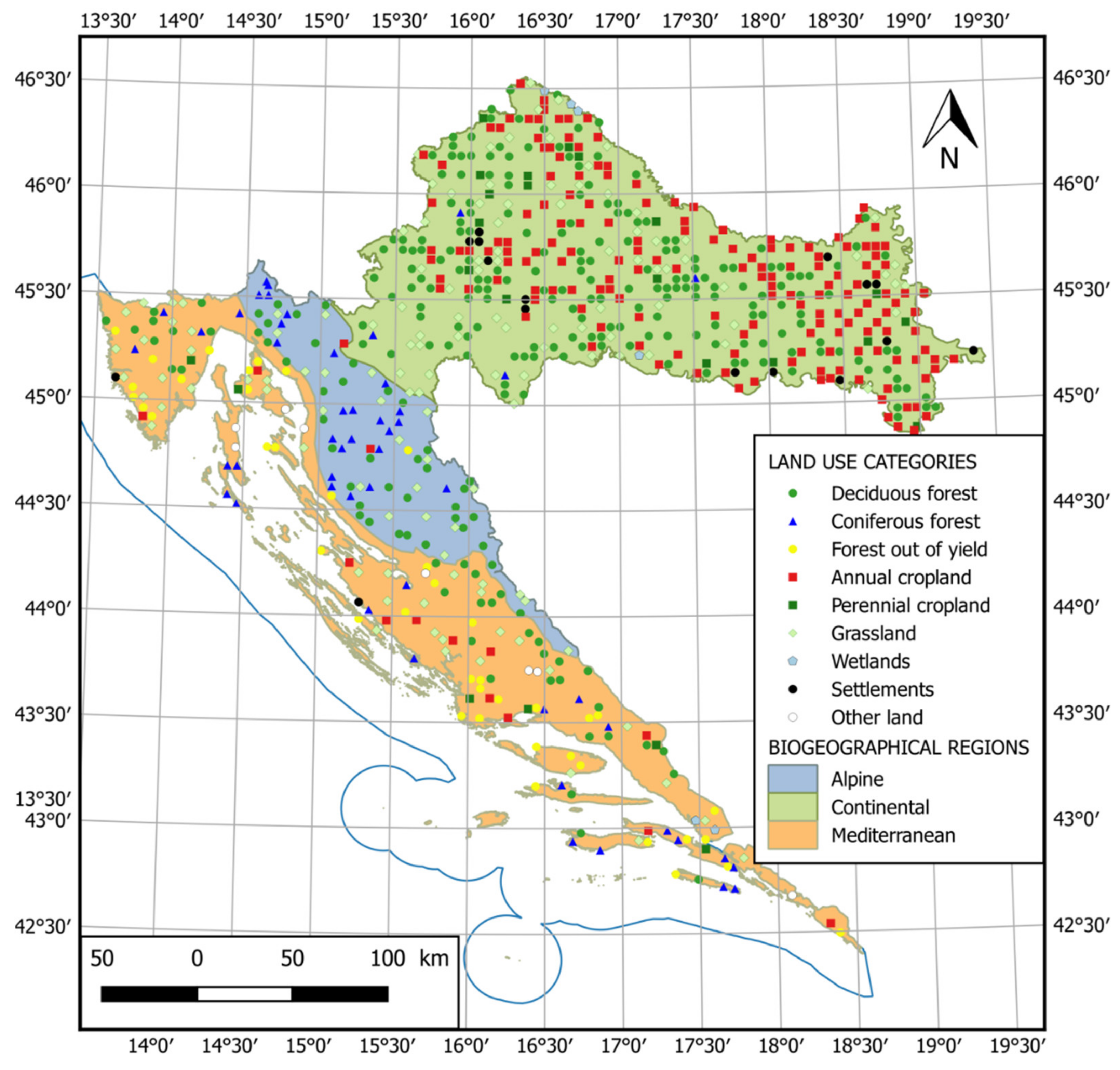
2.1. Study Area

2.2. Field Measurements and Laboratory Analysis
2.3. The Biome-BGCMuSo Model—Parameterisation and Input Data Collection
2.4. Soil Organic Carbon (SOC) Modelling
2.5. Model Evaluation
3. Results
4. Discussion
5. Conclusions
Supplementary Materials
Author Contributions
Funding
Data Availability Statement
Acknowledgments
Conflicts of Interest
Appendix A

| Parameter Name | Parameter Values | References/Remarks | |||
|---|---|---|---|---|---|
| Grassland (1) | Cropland (2) | Deciduous f. (3) | Coniferous f. (4) | ||
| transfer growth period as fraction of growing season | 1 | 1 | 0.3 | 0.3 | |
| litterfall as fraction of growing season | 1 | 1 | 0.3 | 0.3 | |
| base temperature | 5 | 8 | 5 | 5 | proposed value (this study) 1 |
| growing degree day for start of yield allocation | N/A | 825 | 1000 | 1000 | |
| growing degree day of start genetically programmed senescence | N/A | 1680 | 2350 | 2350 | |
| annual leaf and fine root turnover fract. | 1 | 1 | 1 | 0.25 | [67] 4 |
| annual live wood turnover fraction | N/A | N/A | 0.7 | 0.7 | |
| annual whole-plant mortality fraction | 0.05 | 0.02 | 0.02 | 0.005 | [39] 4 |
| annual fire mortality fraction | 0 | 0 | 0 | 0 | |
| new fine root C: new leaf C | 2.5 | 1.02 | 0.95 | 1 | adjusted according to [63] 1, [37] 4 |
| new fruit C: new leaf C | 0 | 0.56 | 0.14 | 0 | proposed value (this study) 4 |
| new softstem C: new leaf C | 0.5 | 2.05 | N/A | N/A | |
| new woody stem C: new leaf C | N/A | N/A | 1.42 | 2.2 | [39] 4 |
| new live wood C: new total wood C | N/A | N/A | 0.16 | 0.1 | [36] 4 |
| new coarse root C: new stem C | N/A | N/A | 0.26 | 0.3 | [36] 4 |
| current growth proportion | 0.5 | 1 | 0.5 | 0.5 | proposed value (this study) 1 |
| C:N of leaves | 25 | 38 | 24.5 | 42 | adjusted according to [64] 2, [39] 4 |
| C:N of leaf litter | 45 | 65 | 47.5 | 93 | [39] 4 |
| C:N of fine roots | 50 | 42 | 43 | 58 | [39] 4 |
| C:N of fruit | 25 | 50 | 33 | 0 | proposed value (this study) 4 |
| C:N of softstem | 25 | 85 | N/A | N/A | |
| C:N of live wood | N/A | N/A | 73.5 | 50 | [39] 4 |
| C:N of dead wood | N/A | N/A | 451 | 729 | [67] 4 |
| leaf litter labile proportion | 0.68 | 0.68 | 0.2 | 0.32 | [36] 4 |
| leaf litter cellulose proportion | 0.23 | 0.23 | 0.56 | 0.44 | [36] 4 |
| fine root litter labile proportion | 0.34 | 0.34 | 0.34 | 0.30 | [36] 4 |
| fine root litter cellulose proportion | 0.44 | 0.44 | 0.44 | 0.45 | [36] 4 |
| fruit litter labile proportion | N/A | 0.68 | 0.3 | 0 | proposed value (this study) 4 |
| fruit litter cellulose proportion | N/A | 0.23 | 0.29 | 0 | proposed value (this study) 4 |
| softstem litter labile proportion | 0.68 | 0.68 | N/A | N/A | |
| softstem litter cellulose proportion | 0.23 | 0.23 | N/A | N/A | |
| dead wood cellulose proportion | N/A | N/A | 0.75 | 0.76 | [36] 4 |
| canopy water interception coefficient | 0.01 | 0.01 | 0.038 | 0.041 | [67] 4 |
| canopy light extinction coefficient | 0.5 | 0.6 | 0.54 | 0.5 | proposed value (this study) 1, [67] 4 |
| all-sided to projected leaf area ratio | 2 | 2 | 2 | 2.6 | [39] 4 |
| canopy average specific leaf area | 49 | 43.3 | 34.5 | 12 | [67] 4 |
| ratio of shaded specific leaf area:sunlit specific leaf area | 2 | 2 | 2 | 2 | |
| fraction of leaf N in Rubisco | 0.2 | 0.39 | 0.088 | 0.04 | proposed value (this study) 1,2, [67] 4 |
| fraction of leaf N in PeP carboxylase | N/A | 0.03 | N/A | N/A | |
| maximum stomatal conductance | 0.004 | 0.012 | 0.0024 | 0.003 | proposed value (this study) 1, [36] 4 |
| cuticular conductance | 0.00006 | 0.00006 | 0.00006 | 0.00001 | [36] 4 |
| boundary layer conductance | 0.04 | 0.04 | 0.005 | 0.08 | [36] 4 |
| relative soil water content limitation1 (proportion to field capacity value) | 1 | 1 | 1 | 1 | proposed value (this study) 3,4 |
| relative soil water content limitation 2 (proportion to saturation capacity value) | 0.99 | 0.99 | 1 | 1 | proposed value (this study) 3,4 |
| vapour pressure deficit: start of conductance reduction | 1000 | 1000 | 200 | 930 | [67] 4 |
| vapour pressure deficit: complete conductance reduction | 5000 | 5000 | 2550 | 4100 | proposed value (this study) 1, [67] 4 |
| senescence mortality coefficient of aboveground plant material | 0.05 | 0.05 | 0.01 | 0 | proposed value (this study) 4 |
| senescence mortality coefficient of belowground plant material | 0.01 | 0.01 | 0.01 | 0 | proposed value (this study) 4 |
| genetically programmed senescence mortality coefficient of leaf | 0 | 0.1 | 0.025 | 0 | proposed value (this study) 4 |
| turnover rate of wilted standing biomass to litter | 0.01 | 0.001 | 0.01 | 0.01 | proposed value (this study) 1 |
| turnover rate of cut-down non-woody biomass to litter | 0.05 | 0.01 | 0.05 | 0.05 | proposed value (this study) 1 |
| N denitrification proportion | 0.01 | 0.01 | 0.01 | 0.01 | |
| bulk N denitrification proportion, wet case | 0.005 | 0.005 | 0.02 | 0.02 | proposed value (this study) 1,2 |
| bulk N denitrification proportion, dry case | 0.001 | 0.001 | 0.01 | 0.01 | proposed value (this study) 1,2 |
| mobile N proportion (leaching) | 0.1 | 0.1 | 0.1 | 0.1 | |
| symbiotic+asymbiotic fixation of N | 0.003 | 0.0005 | 0.0036 | 0.0016 | adjusted according to [65,66] 1, [65] 4 |
| ratio of storage and actual pool mortality due to management | 0.1 | 0.1 | 0.9 | 0.9 | |
| critical value of soilstress coefficient | 0.3 | 0.4 | 0.5 | 0.3 | proposed value (this study) 1,4 |
| critical number of stress days | 60 | 60 | 90 | 90 | |
| maximum depth of rooting zone | 0.1–0.63 | 0.1–0.63 | 0.1–0.63 | 0.1–0.63 | plot-specific |
| root distribution parameter | 3.67 | 3.67 | 3.67 | 3.67 | |
| maturity coefficient | 0.5 | 0.5 | 0.5 | 0.5 | |
| growth respiration per unit of C grown | 0.3 | 0.3 | 0.3 | 0.3 | |
| maintenance respiration in kgC/day per kg of tissue N | 0.218 | 0.218 | 0.4 | 0.4 | |
| Land-Use Category | Management Activity | DOY | Description |
|---|---|---|---|
| Deciduous forests Coniferous forests | Thinning * | 30 | 2.1% y−1 3% y−1 |
| Grassland | fertilising | 100, 190 | 30 + 30 kg N ha−1 y−1 animal manure (2% N, 40% C) |
| Mowing | 150, 200 | 75% plant material | |
| Annual cropland | Planting | 105 | 25 kg ha−1 |
| fertilising | 91, 145, 288 | 60 + 40 + 50 kg N ha−1 y−1 70% chemical fertiliser (47% N, 5% C) 30% animal manure | |
| Harvesting | 273 | 50% plant material | |
| Ploughing | 300 | down to 30 cm |


References
- UN (United Nations). Kyoto Protocol to the United Nations Framework Convention on Climate Change; United Nations: Kyoto, Japan, 1997; pp. 1–21. Available online: https://unfccc.int/resource/docs/cop3/07a01.pdf (accessed on 23 July 2021).
- UN (United Nations). Paris Agreement; United Nations: Paris, France, 2015; pp. 1–27. Available online: https://undocs.org/en/FCCC/CP/2015/10/Add.1 (accessed on 23 July 2021).
- EC (European Commission). Communication from the Commission to the European Parliament, the European Council, the Council, the European Economic and Social Committee and the Committee of the Regions-The European Green Deal; European Commission: Brussels, Belgium, 2019; pp. 1–24. [Google Scholar]
- Batjes, N.H. Total C and N in soils of the world. Eur. J. Soil Sci. 1996, 47, 151–163. [Google Scholar] [CrossRef]
- Scharlemann, J.P.W.; Tanner, E.V.J.; Hiederer, R.; Kapos, V. Global soil carbon: Understanding and managing the largest terrestrial carbon pool. Carbon Manag. 2014, 5, 81–91. [Google Scholar] [CrossRef]
- Crowther, T.W.; Todd-Brown, K.E.O.; Rowe, C.W.; Wieder, W.R.; Carey, J.C.; Machmuller, M.B.; Snoek, B.L.; Fang, S.; Zhou, G.; Allison, S.D.; et al. Quantifying global soil carbon losses in response to warming. Nature 2016, 540, 104–108. [Google Scholar] [CrossRef] [PubMed]
- Rustad, L.E.; Campbell, J.L.; Marion, G.M.; Norby, R.J.; Mitchell, M.J.; Hartley, A.E.; Cornelissen, J.H.C.; Gurevitch, J. Gcte-News. A meta-analysis of the response of soil respiration, net nitrogen mineralization, and aboveground plant growth to experimental ecosystem warming. Oecologia 2001, 126, 543–562. [Google Scholar] [CrossRef] [PubMed]
- Melillo, J.M.; Steudler, P.A.; Aber, J.D.; Newkirk, K.; Lux, H.; Bowles, F.P.; Catricala, C.; Magill, A.; Ahrens, T.; Morrisseau, S. Soil warming and carbon-cycle feedbacks to the climate system. Science 2002, 298, 2173–2176. [Google Scholar] [CrossRef] [PubMed]
- Fyson, C.L.; Jeffery, M.L. Ambiguity in the land use component of mitigation contributions toward the Paris agreement goals. Earths Future 2019, 7, 873–891. [Google Scholar] [CrossRef]
- IPCC GPG (The Intergovernmental Panel on Climate Change Good Practice Guidelines). Guidelines for National Greenhouse Gas Inventories; Eggleston, H.S., Buendia, L., Miwa, K., Ngara, T., Tanabe, K., Eds.; National Greenhouse Gas Inventories Programme, IGES: Kanagawa, Japan, 2006. [Google Scholar]
- Jenkinson, D.S.; Coleman, K. The turnover of organic carbon in subsoils. Part 2. Modelling carbon turnover. Eur. J. Soil Sci. 2008, 59, 400–413. [Google Scholar] [CrossRef]
- UK NIR. United Kingdom National Inventory Report 2020. Available online: https://unfccc.int/documents/225987 (accessed on 23 July 2021).
- Liski, J.; Palosuo, T.; Peltoniemi, M.; Sievanen, R. Carbon and decomposition model Yasso for forest soils. Ecol. Modell. 2005, 189, 168–182. [Google Scholar] [CrossRef]
- Alvaro-Fuentes, J.; Easter, M.; Cantero-Martinez, C.; Paustian, K. Modelling soil organic carbon stocks and their changes in the northeast of Spain. Eur. J. Soil Sci. 2011, 62, 685–695. [Google Scholar] [CrossRef] [Green Version]
- CH NIR. Swiss National Inventory Report 2020. Available online: https://unfccc.int/documents/224855 (accessed on 23 July 2021).
- FI NIR. Finnish National Inventory Report 2020. Available online: https://unfccc.int/documents/219060 (accessed on 23 July 2021).
- Parton, J.W. The century model. In Evaluation of Soil Organic Matter Models; Powlson, D.S., Smith, P., Smith, J.U., Eds.; Springer: Berlin/Heidelberg, Germany, 1996; pp. 283–291. [Google Scholar]
- Falloon, P.; Smith, P. Accounting for changes in soil carbon under the Kyoto Protocol: Need for improved long-term data sets to reduce uncertainty in model projections. Soil Use Manag. 2003, 19, 265–269. [Google Scholar] [CrossRef]
- Hararuk, O.; Xia, J.Y.; Luo, Y.Q. Evaluation and improvement of a global land model against soil carbon data using a Bayesian Markov chain Monte Carlo method. J. Geophys. Res. Biogeosci. 2014, 119, 403–417. [Google Scholar] [CrossRef]
- Tupek, B.; Launiainen, S.; Peltoniemi, M.; Sievanen, R.; Perttunen, J.; Kulmala, L.; Penttila, T.; Lindroos, A.J.; Hashimoto, S.; Lehtonen, A. Evaluating CENTURY and Yasso soil carbon models for CO2 emissions and organic carbon stocks of boreal forest soil with Bayesian multi-model inference. Eur. J. Soil Sci. 2019, 70, 847–858. [Google Scholar]
- Luo, Y.; Zhou, X. Soil Respiration and the Environment; Elsevier: Amsterdam, The Netherlands, 2006; p. 316. [Google Scholar]
- Campbell, E.E.; Paustian, K. Current developments in soil organic matter modelling and the expansion of model applications: A review. Environ. Res. Lett. 2015, 10, 123004. [Google Scholar] [CrossRef]
- Parton, W.; Del Grosso, S.J.; Plante, A.F.; Adair, E.C.; Lutz, S.M. Modelling the dynamics of soil organic matter and nutrient cycling. In Soil Microbiology, Ecology, and Biochemistry, 4th ed.; Paul, E.A., Ed.; Elsevier: Amsterdam, The Netherlands, 2015; pp. 505–537. [Google Scholar]
- Keel, S.G.; Leifeld, J.; Mayer, J.; Taghizadeh-Toosi, A.; Olesen, J.E. Large uncertainty in soil carbon modelling related to method of calculation of plant carbon input in agricultural systems. Eur. J. Soil Sci. 2017, 68, 953–963. [Google Scholar] [CrossRef] [Green Version]
- Ostle, N.J.; Levy, P.E.; Evans, C.D.; Smith, P. UK land use and soil carbon sequestration. Land Use Policy 2009, 26, S274–S283. [Google Scholar] [CrossRef]
- Poeplau, C.; Don, A.; Vesterdal, L.; Leifeld, J.; Van Wesemael, B.; Schumacher, J.; Gensior, A. Temporal dynamics of soil organic carbon after land-use change in the temperate zone-carbon response functions as a model approach. Glob. Change Biol. 2011, 17, 2415–2427. [Google Scholar] [CrossRef]
- Johnson, D.W.; Curtis, P.S. Effects of forest management on soil C and N storage: Meta analysis. For. Ecol Manag. 2001, 140, 227–238. [Google Scholar] [CrossRef]
- Chen, L.C.; Wang, S.L.; Wang, Q.K. Ecosystem carbon stocks in a forest chronosequence in Hunan Province, South China. Plant Soil 2016, 409, 217–228. [Google Scholar] [CrossRef]
- Ostrogović Sever, M.Z.; Alberti, G.; Delle Vedove, G.; Marjanović, H. Temporal Evolution of carbon stocks, fluxes and carbon balance in pedunculate oak chronosequence under close-to-nature forest management. Forests 2019, 10, 814. [Google Scholar] [CrossRef] [Green Version]
- Smith, J.; Smith, P.; Wattenbach, M.; Zaehle, S.; Hiederer, R.; Jones, R.J.A.; Montanarella, L.; Rounsevell, M.D.A.; Reginster, I.; Ewert, F. Projected changes in mineral soil carbon of European croplands and grasslands, 1990–2080. Glob. Change Biol. 2005, 11, 2141–2152. [Google Scholar] [CrossRef]
- Mondini, C.; Coleman, K.; Whitmore, A.P. Spatially explicit modelling of changes in soil organic C in agricultural soils in Italy, 2001–2100: Potential for compost amendment. Agric. Ecosyst. Environ. 2012, 153, 24–32. [Google Scholar] [CrossRef]
- Munoz-Rojas, M.; Jordan, A.; Zavala, L.M.; Gonzalez-Penaloza, F.A.; De la Rosa, D.; Pino-Mejias, R.; Anaya-Romero, M. Modelling soil organic carbon stocks in global change scenarios: A CarboSOIL application. Biogeosciences 2013, 10, 8253–8268. [Google Scholar] [CrossRef] [Green Version]
- Running, S.W.; Hunt, E.R.J. Generalization of a forest ecosystem process model for other biomes, BIOME-BGC, and an application for global-scale models. In Scaling Physiological Processes: Leaf to Globe; Ehleringer, J.R., Field, C., Eds.; Academic Press: San Diego, CA, USA, 1993; pp. 141–158. [Google Scholar]
- Hidy, D.; Barcza, Z.; Marjanovic, H.; Sever, M.Z.O.; Dobor, L.; Gelybo, G.; Fodor, N.; Pinter, K.; Churkina, G.; Running, S.; et al. Terrestrial ecosystem process model Biome-BGCMuSo v4.0: Summary of improvements and new modeling possibilities. Geosci. Model Dev. 2016, 9, 4405–4437. [Google Scholar] [CrossRef] [Green Version]
- Pietsch, S.A.; Hasenauer, H. Using mechanistic modeling within forest ecosystem restoration. For. Ecol. Manag. 2002, 159, 111–131. [Google Scholar] [CrossRef]
- Bond-Lamberty, B.; Gower, S.T.; Ahl, D.E.; Thornton, P.E. Reimplementation of the Biome-BGC model to simulate successional change. Tree Physiol. 2005, 25, 413–424. [Google Scholar] [CrossRef] [PubMed] [Green Version]
- Cienciala, E.; Tatarinov, F.A. Application of BIOMEBGC model to managed forests. 2. Comparison with longterm observations of stand production for major tree species. For. Ecol. Manag. 2006, 237, 252–266. [Google Scholar] [CrossRef]
- Hidy, D.; Barcza, Z.; Haszpra, L.; Churkina, G.; Pinter, K.; Nagy, Z. Development of the Biome-BGC model for simulation of managed herbaceous ecosystems. Ecol. Model 2012, 226, 99–119. [Google Scholar] [CrossRef]
- White, M.; Thornton, P.E.; Running, S.W.; Nemani, R.R. Parameterization and sensitivity analysis of the BIOME-BGC terrestrial ecosystem model: Net primary production controls. Earth Interact. 2000, 4, 1–85. [Google Scholar] [CrossRef]
- Pietsch, S.A.; Hasenauer, H.; Thornton, P.E. BGC-model parameters for tree species growing in central European forests. For. Ecol. Manag. 2005, 211, 264–295. [Google Scholar] [CrossRef]
- Trusilova, K.; Trembath, J.; Churkina, G. Parameter Estimation and Validation of the Terrestrial Ecosystem Model Biome-Bgc Using Eddy-Covariance Flux Measurements; MPI for Biogeochemistry: Jena, Germany, 2010; Volume 2009. [Google Scholar]
- Wu, Y.; Wang, X.; Ouyang, S.; Xu, K.; Hawkins, B.A.; Sun, O.J. A test of Biome-BGC with dendrochronology for forests along the altitudinal gradient of Mt. Changbai in northeast. Chin. J. Plant Ecol. 2017, 10, 415–425. [Google Scholar] [CrossRef] [Green Version]
- Hlasny, T.; Barcza, Z.; Fabrika, M.; Balazs, B.; Churkina, G.; Pajtik, J.; Sedmak, R.; Turcani, M. Climate change impacts on growth and carbon balance of forests in Central Europe. Clim. Res. 2011, 47, 219–236. [Google Scholar] [CrossRef] [Green Version]
- Han, Q.F.; Luo, G.P.; Li, C.F.; Shakir, A.; Wu, M.; Saidov, A. Simulated grazing effects on carbon emission in Central Asia. Agric. For. Meteorol. 2016, 216, 203–214. [Google Scholar] [CrossRef]
- Hartig, F.; Dyke, J.; Hickler, T.; Higgins, S.I.; O’Hara, R.B.; Scheiter, S.; Huth, A. Connecting dynamic vegetation models to data-an inverse perspective. J. Biogeogr. 2012, 39, 2240–2252. [Google Scholar] [CrossRef]
- Sitch, S.; Smith, B.; Prentice, I.C.; Arneth, A.; Bondeau, A.; Cramer, W.; Kaplan, J.O.; Levis, S.; Lucht, W.; Sykes, M.T.; et al. Evaluation of ecosystem dynamics, plant geography and terrestrial carbon cycling in the LPJ dynamic global vegetation model. Glob. Change Biol. 2003, 9, 161–185. [Google Scholar] [CrossRef]
- Lasch-Born, P.; Suckow, F.; Reyer, C.P.O.; Gutsch, M.; Kollas, C.; Badeck, F.W.; Bugmann, H.K.M.; Grote, R.; Furstenau, C.; Lindner, M.; et al. Description and evaluation of the process-based forest model 4C v2.2 at four European forest sites. Geosci. Model Dev. 2020, 13, 5311–5343. [Google Scholar] [CrossRef]
- AT NIR. Austrian National Inventory Report 2020. Available online: https://unfccc.int/documents/226418 (accessed on 23 July 2021).
- Bai, J.W.; Shen, Z.Y.; Yan, T.Z. A comparison of single-and multi-site calibration and validation: A case study of SWAT in the Miyun Reservoir watershed, China. Front. Earth Sci. 2017, 11, 592–600. [Google Scholar] [CrossRef]
- Forrester, D.I.; Hobi, M.L.; Mathys, A.S.; Stadelmann, G.; Trotsiuk, V. Calibration of the process-based model 3-PG for major central European tree species. Eur. J. For. Res. 2021, 140, 1–22. [Google Scholar] [CrossRef]
- EEA (European Environmental Agency). Biogeographical Regions in Europe; EEA: Copenhagen, Denmark, 2016; Available online: https://www.eea.europa.eu/data-and-maps/figures/biogeographical-regions-in-europe-2 (accessed on 23 July 2021).
- Zaninović, K.; Gajić-Čapka, M.; Perčec Tadić, M.; Vučetić, M.; Milković, J.; Bajić, A.; Cindrić, K.; Cvitan, L.; Katušin, Z.; Kaučić, D.; et al. Climate Atlas of Croatia 1961–1990, 1971–2000; Meteorological and Hydrological Service: Zagreb, Croatia, 2008; p. 200. [Google Scholar]
- Seletković, Z.; Katušin, Z. Climate of Croatia. In Forests of Croatia; Rauš, Đ., Ed.; Faculty of Forestry, University of Zagreb, Croatian Forests Ltd.: Zagreb, Croatia, 1992; pp. 13–18. [Google Scholar]
- Bogunović, M.; Vidaček, Ž.; Racz, Z.; Husnjak, S.; Sraka, M. The practical aspects of soil suitability map of Croatia. Agron. Glas. 1997, 59, 363–399. Available online: https://hrcak.srce.hr/147226 (accessed on 23 July 2021).
- Bašić, F.; Bogunović, M.; Božić, M.; Husnjak, S.; Jurić, I.; Kisić, I.; Mesić, M.; Mirošević, N.; Romić, D.; Žugec, I. Regionalisation of Croatian agriculture. Agric. Conspec. Sci. 2007, 72, 27–38. [Google Scholar]
- Velić, I.; Vlahović, I. Explanatory Notes of the Geological Map of the Republic of Croatia in 1:300,000 Scale; Croatian Geological Survey: Zagreb, Croatia, 2009; p. 147. [Google Scholar]
- Halamić, J.; Miko, S. Geochemical Atlas of the Republic of Croatia; Croatian Geological Survey: Zagreb, Croatia, 2009; p. 87. [Google Scholar]
- Croatian Forests Ltd. Forest Management Area Plan for the Republic of Croatia for the Period 2016–2025; Croatian Forests Ltd: Zagreb, Croatia, 2016; Available online: https://poljoprivreda.gov.hr/istaknute-teme/sume-112/sumarstvo/sumskogospodarska-osnova-2016-2025/250 (accessed on 23 July 2021).
- HR NIR. Croatian National Inventory Report 2020. Available online: https://unfccc.int/documents/223243 (accessed on 23 July 2021).
- Koven, C.D.; Riley, W.J.; Subin, Z.M.; Tang, J.Y.; Torn, M.S.; Collins, W.D.; Bonan, G.B.; Lawrence, D.M.; Swenson, S.C. The effect of vertically resolved soil biogeochemistry and alternate soil C and N models on C dynamics of CLM4. Biogeosciences 2013, 10, 7109–7131. [Google Scholar] [CrossRef] [Green Version]
- Falloon, P.D.; Smith, P. Modelling refractory soil organic matter. Biol. Fertil. Soils 2000, 30, 388–398. [Google Scholar]
- Dobor, L.; Barcza, Z.; Hlasny, T.; Havasi, A.; Horvath, F.; Ittzes, P.; Bartholy, J. Bridging the gap between climate models and impact studies: The FORESEE Database. Geosci. Data J. 2014, 2, 1–11. [Google Scholar] [CrossRef] [PubMed]
- Dalrymple, R.L.; Dwyer, D.D. Root and shoot growth of five range grasses. J. Range Manag. 1967, 20, 141–145. [Google Scholar] [CrossRef]
- Barbosa, J.Z.; Ferreira, C.F.; dos Santos, N.Z.; Motta, A.C.V.; Prior, S.; Gabardo, J. Production, carbon and nitrogen in stover fractions of corn (Zea mays L.) in response to cultivar development. Cienc. Agrotecnologia 2016, 40, 665–675. [Google Scholar] [CrossRef] [Green Version]
- Cleveland, C.C.; Townsend, A.R.; Schimel, D.S.; Fisher, H.; Howarth, R.W.; Hedin, L.O.; Perakis, S.S.; Latty, E.F.; Von Fischer, J.C.; Elseroad, A.; et al. Global patterns of terrestrial biological nitrogen (N-2) fixation in natural ecosystems. Glob. Biogeochem. Cycles 1999, 13, 623–645. [Google Scholar] [CrossRef] [Green Version]
- Butler, G.J.; Christian, T.; Schwenke, G.D.; Herridge, D.F. Nitrogen fixation inputs from lucerne-dominated pastures in the Central-East of NSW. In Farming Systems, Proceedings of the 10th Agronomy Conference, Hobart, TAS, Australia, 21 January–1 February 2001; Rowe, B., Donaghy, D., Mendham, N., Eds.; Agronomy Australia Proceedings: Toowoomba, Australia, 2001; Available online: http://www.agronomyaustraliaproceedings.org/images/sampledata/2001/p/1/butler.pdf (accessed on 23 July 2021).
- Thornton, P.E.; Running, S.W.; Hunt, E.R. Biome-BGC: Terrestrial Ecosystem Process Model, Version 4.1.1; ORNL DAAC: Oak Ridge, TN, USA, 2005; Available online: https://daac.ornl.gov/cgi-bin/dsviewer.pl?ds_id=805 (accessed on 23 July 2021).
- Mauna Loa Observatory. Available online: http://www.esrl.noaa.gov/gmd/obop/mlo/ (accessed on 23 July 2021).
- Etheridge, D.M.; Steele, L.P.; Langenfelds, R.L.; Francey, R.J.; Barnola, J.M.; Morgan, V.I. Natural and anthropogenic changes in atmospheric CO2 over the last 1000 years from air in Antarctic ice and firn. J. Geophys. Res. Atmos. 1996, 101, 4115–4128. [Google Scholar] [CrossRef] [Green Version]
- Churkina, G.; Brovkin, V.; von Bloh, W.; Trusilova, K.; Jung, M.; Dentener, F. Synergy of rising nitrogen depositions and atmospheric CO2 on land carbon uptake moderately offsets global warming. Glob. Biogeochem. Cycles 2009, 23, GB4027. [Google Scholar] [CrossRef] [Green Version]
- Thornton, P.E.; Rosenbloom, N.A. Ecosystem model spin-up: Estimating steady state conditions in a coupled terrestrial carbon and nitrogen cycle model. Ecol. Model 2005, 189, 25–48. [Google Scholar] [CrossRef]
- Hidy, D.; Barcza, Z.; Thornton, P.; Running, S. User’s Guide for Biome-BGC MuSo 4.0. 2016. Available online: http://nimbus.elte.hu/bbgc/files/Manual_BBGC_MuSo_v4.0.pdf (accessed on 23 July 2021).
- Ostrogović Sever, M.Z.; Paladinić, E.; Barcza, Z.; Hidy, D.; Kern, A.; Anić, M.; Marjanović, H. Biogeochemical Modelling vs. tree-ring measurements-comparison of growth dynamic estimates at two distinct oak forests in Croatia. South-East Eur. For. 2017, 8, 71–84. [Google Scholar] [CrossRef]
- Thornton, P.E.; Law, B.E.; Gholz, H.L.; Clark, K.L.; Falge, E.; Ellsworth, D.S.; Golstein, A.H.; Monson, R.K.; Hollinger, D.; Falk, M.; et al. Modeling and measuring the effects of disturbance history and climate on carbon and water budgets in evergreen needleleaf forests. Agric. For. Meteorol. 2002, 113, 185–222. [Google Scholar] [CrossRef]
- Merganicova, K.; Pietsch, S.A.; Hasenauer, H. Testing mechanistic modeling to assess impacts of biomass removal. For. Ecol. Manag. 2005, 207, 37–57. [Google Scholar] [CrossRef]
- Chiesi, M.; Maselli, F.; Moriondo, M.; Fibbi, L.; Bindi, M.; Running, S.W. Application of BIOME-BGC to simulate Mediterranean forest processes. Ecol. Model 2007, 206, 179–190. [Google Scholar] [CrossRef]
- Ueyama, M.; Ichii, K.; Hirata, R.; Takagi, K.; Asanuma, J.; Machimura, T.; Nakai, Y.; Ohta, T.; Saigusa, N.; Takahashi, Y.; et al. Simulating carbon and water cycles of larch forests in East Asia by the BIOME-BGC model with AsiaFlux data. Biogeosciences 2010, 7, 959–977. [Google Scholar] [CrossRef] [Green Version]
- Maselli, F.; Chiesi, M.; Brilli, L.; Moriondo, M. Simulation of olive fruit yield in Tuscany through the integration of remote sensing and ground data. Ecol. Model 2012, 244, 1–12. [Google Scholar] [CrossRef]
- Morais, T.G.; Teixeira, R.F.M.; Domingos, T. Detailed global modelling of soil organic carbon in cropland, grassland and forest soils. PLoS ONE 2019, 14, e0222604. [Google Scholar] [CrossRef] [PubMed] [Green Version]
- Bakker, M.M.; Hatna, E.; Kuhlman, T.; Mucher, C.A. Changing environmental characteristics of European cropland. Agric. Syst. 2011, 104, 522–532. [Google Scholar] [CrossRef]
- Smith, W.K.; Hinckley, T.M. Ecophysiology of Coniferous Forests, 1st ed.; Academic Press: San Diego, CA, USA, 1995; p. 338. [Google Scholar]
- Muller, T.; Hoper, H. Soil organic matter turnover as a function of the soil clay content: Consequences for model applications. Soil Biol. Biochem. 2004, 36, 877–888. [Google Scholar] [CrossRef]
- Rasse, D.P.; Rumpel, C.; Dignac, M.F. Is soil carbon mostly root carbon? Mechanisms for a specific stabilisation. Plant Soil 2005, 269, 341–356. [Google Scholar] [CrossRef]
- Tatarinov, F.A.; Cienciala, E. Application of BIOME-BGC model to managed forests 1. Sensitivity analysis. For. Ecol. Manag. 2006, 237, 267–279. [Google Scholar] [CrossRef]
- Merganicova, K.; Merganic, J.; Lehtonen, A.; Vacchiano, G.; Sever, M.Z.O.; Augustynczik, A.L.D.; Grote, R.; Kyselova, I.; Makela, A.; Yousefpour, R.; et al. Forest carbon allocation modelling under climate change. Tree Physiol. 2019, 39, 1937–1960. [Google Scholar] [CrossRef] [PubMed]
- Van Noordwijk, M.; van de Geijn, S.C. Root, shoot and soil parameters required for process-oriented models of crop growth limited by water or nutrients. Plant Soil 1996, 183, 1–25. [Google Scholar] [CrossRef]
- Mokany, K.; Raison, R.J.; Prokushkin, A.S. Critical analysis of root: Shoot ratios in terrestrial biomes. Glob. Change Biol. 2006, 12, 84–96. [Google Scholar] [CrossRef]
- Friedlingstein, P.; Joel, G.; Field, C.B.; Fung, I.Y. Toward an allocation scheme for global terrestrial carbon models. Glob. Change Biol. 1999, 5, 755–770. [Google Scholar] [CrossRef]
- Jochheim, H.; Puhlmann, M.; Beese, F.; Berthold, D.; Einert, P.; Kallweit, R.; Konopatzky, A.; Meesenburg, H.; Meiwes, K.J.; Raspe, S.; et al. Modelling the carbon budget of intensive forest monitoring sites in Germany using the simulation model BIOME-BGC. Iforest 2009, 2, 7–10. [Google Scholar] [CrossRef]
- Viskari, T.; Laine, M.; Kulmala, L.; Makela, J.; Fer, I.; Liski, J. Improving Yasso15 soil carbon model estimates with ensemble adjustment Kalman filter state data assimilation. Geosci. Model Dev. 2020, 13, 5959–5971. [Google Scholar] [CrossRef]
- Post, J.; Hattermann, F.F.; Krysanova, V.; Suckow, F. Parameter and input data uncertainty estimation for the assessment of long-term soil organic carbon dynamics. Environ. Model. Softw. 2008, 23, 125–138. [Google Scholar] [CrossRef]
- Fodor, N.; Pasztor, L.; Szabo, B.; Laborczi, A.; Pokovai, K.; Hidy, D.; Hollos, R.; Kristof, E.; Kis, A.; Dobor, L.; et al. Input database related uncertainty of Biome-BGCMuSo agro-environmental model outputs. Int. J. Digit. Earth 2021, 1–20. [Google Scholar] [CrossRef]
- Mao, Z.; Derrien, D.; Didion, M.; Liski, J.; Eglin, T.; Nicolas, M.; Jonard, M.; Saint-Andre, L. Modeling soil organic carbon dynamics in temperate forests with Yasso07. Biogeosciences 2019, 16, 1955–1973. [Google Scholar] [CrossRef] [Green Version]
- Smallman, T.L.; Milodowski, D.T.; Neto, E.S.; Koren, G.; Ometto, J.; Williams, M. Parameter uncertainty dominates C cycle forecast errors over most of Brazil for the 21st Century. Earth Syst. Dyn. Discuss. 2021, 1–52. [Google Scholar] [CrossRef]
- Jung, M.; Vetter, M.; Herold, M.; Churkina, G.; Reichstein, M.; Zaehle, S.; Ciais, P.; Viovy, N.; Bondeau, A.; Chen, Y.; et al. Uncertainties of modeling gross primary productivity over Europe: A systematic study on the effects of using different drivers and terrestrial biosphere models. Glob. Biogeochem. Cycles 2007, 21, GB4021. [Google Scholar] [CrossRef]
- Soudzilovskaia, N.A.; van Bodegom, P.M.; Terrer, C.; van’t Zelfde, M.; McCallum, I.; McCormack, M.L.; Fisher, J.B.; Brundrett, M.C.; de Sa, N.C.; Tedersoo, L. Global mycorrhizal plant distribution linked to terrestrial carbon stocks. Nat. Commun. 2019, 10, 1–10. [Google Scholar] [CrossRef] [PubMed] [Green Version]
- Hararuk, O.; Smith, M.J.; Luo, Y.Q. Microbial models with data-driven parameters predict stronger soil carbon responses to climate change. Glob. Change Biol. 2015, 21, 2439–2453. [Google Scholar] [CrossRef] [PubMed]
- Filser, J.; Faber, J.H.; Tiunov, A.V.; Brussaard, L.; Frouz, J.; De Deyn, G.; Uvarov, A.V.; Berg, M.P.; Lavelle, P.; Loreau, M.; et al. Soil fauna: Key to new carbon models. Soil 2016, 2, 565–582. [Google Scholar] [CrossRef] [Green Version]


| LU Category | National Inventory Report Categories | Area in 2016 (kha) | Share (%) |
|---|---|---|---|
| Forest land | Deciduous forests | 1618.3 | 28.6% |
| Coniferous forests | 209.4 | 3.7% | |
| Forests out of yield | 484.7 | 8.6% | |
| Cropland | Annual cropland | 1386.0 | 24.5% |
| Perennial cropland | 105.1 | 1.9% | |
| Grassland | Grassland | 1096.6 | 19.4% |
| Wetlands | Wetlands | 74.1 | 1.3% |
| Settlements | Settlements | 203.6 | 3.6% |
| Other land | Other land | 238.2 | 4.2% |
| Land-use change | Land-use change | 243.3 | 4.3% |
| TOTAL | 5659.4 | 100.0% | |
| LU Category | N | Measured SOC30 | Modelled SOC30 | ||
|---|---|---|---|---|---|
| t C ha−1 | CV (%) | t C ha−1 | CV (%) | ||
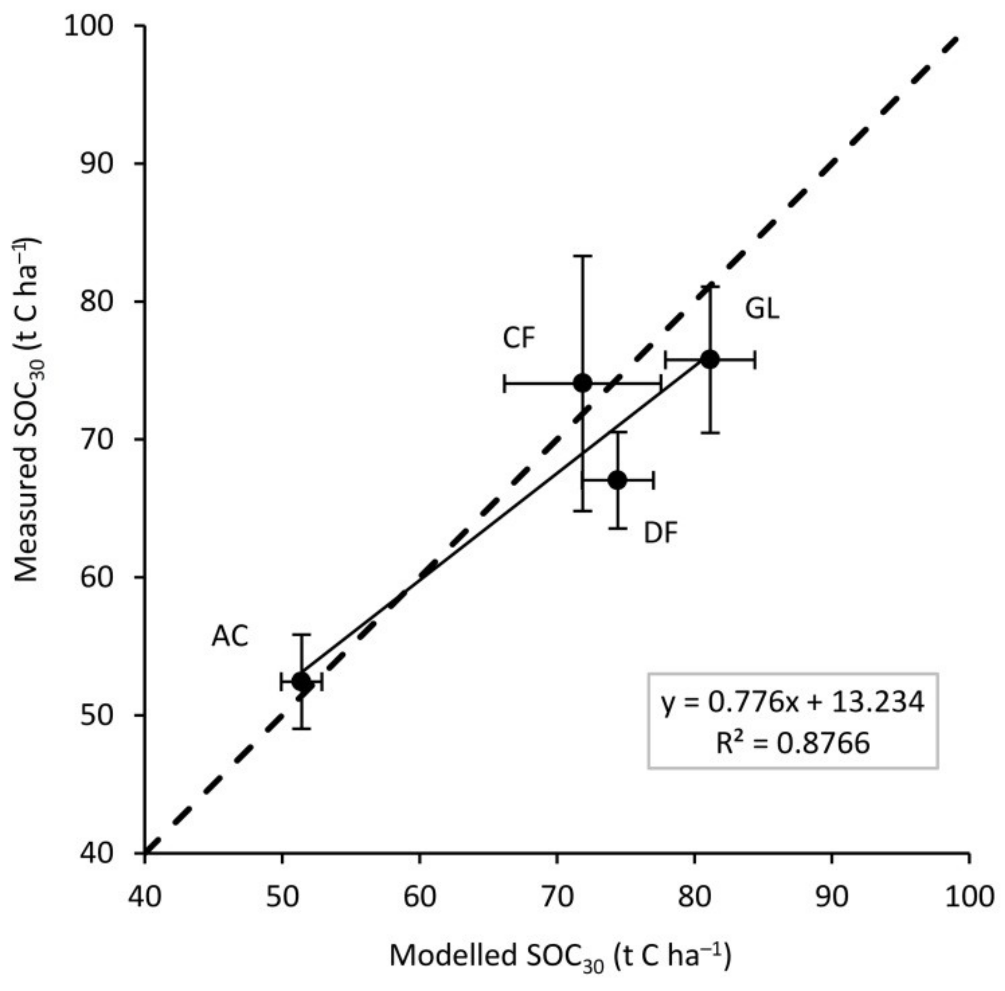
| Deciduous forests (DF) | 241 | 67.04 ± 1.78 | 41 | 74.42 ± 1.32 | 28 |
| Coniferous forests (CF) | 51 | 74.05 ± 4.71 | 45 | 71.86 ± 2.90 | 29 |
| Annual croplands (AC) | 161 | 52.44 ± 1.74 | 42 | 51.41 ± 0.75 | 19 |
| Grasslands (GL) | 120 | 75.77 ± 2.70 | 39 | 81.14 ± 1.66 | 22 |
| Total | 573 | 65.39 ± 1.19 | 44 | 69.13 ± 0.88 | 30 |
| LU Category in NIR | Biogeographical Region | N | Measured SOC0–30 cm | Modelled SOC0–30 cm | ||
|---|---|---|---|---|---|---|
| AV ± SE | CV (%) | AV ± SE | CV (%) | |||
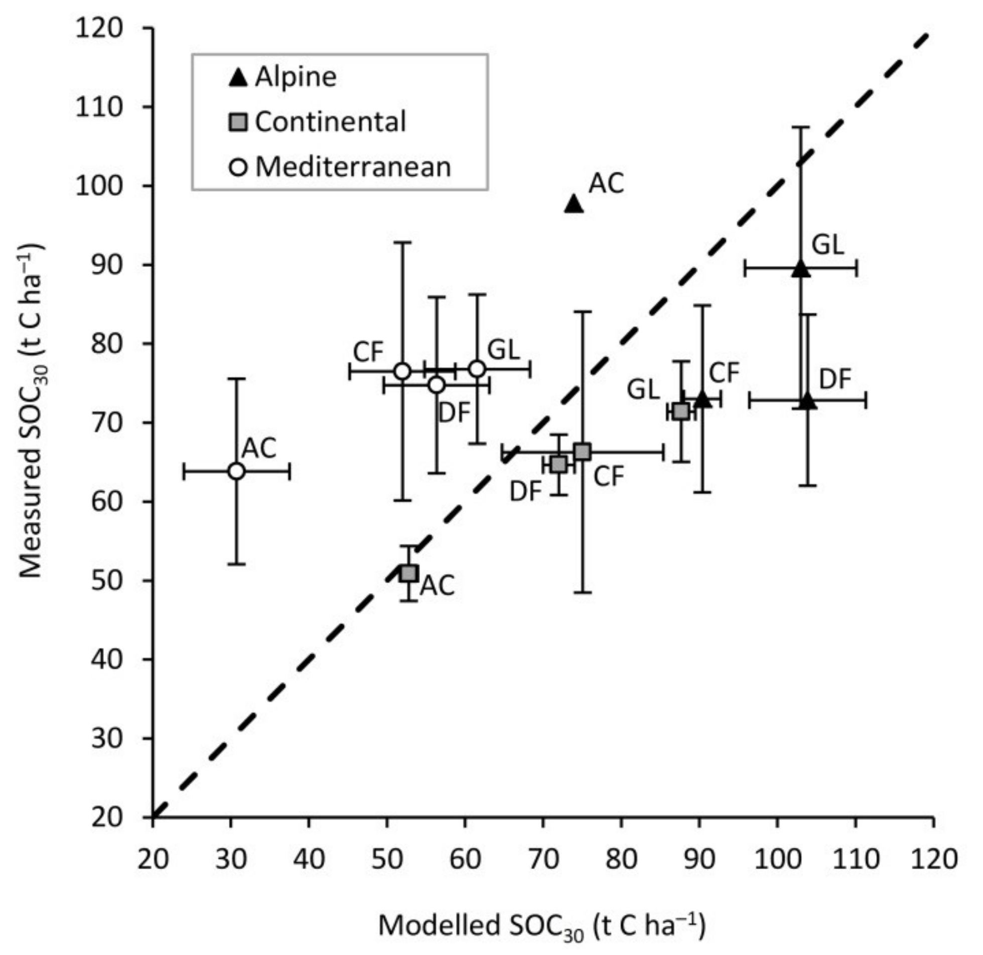
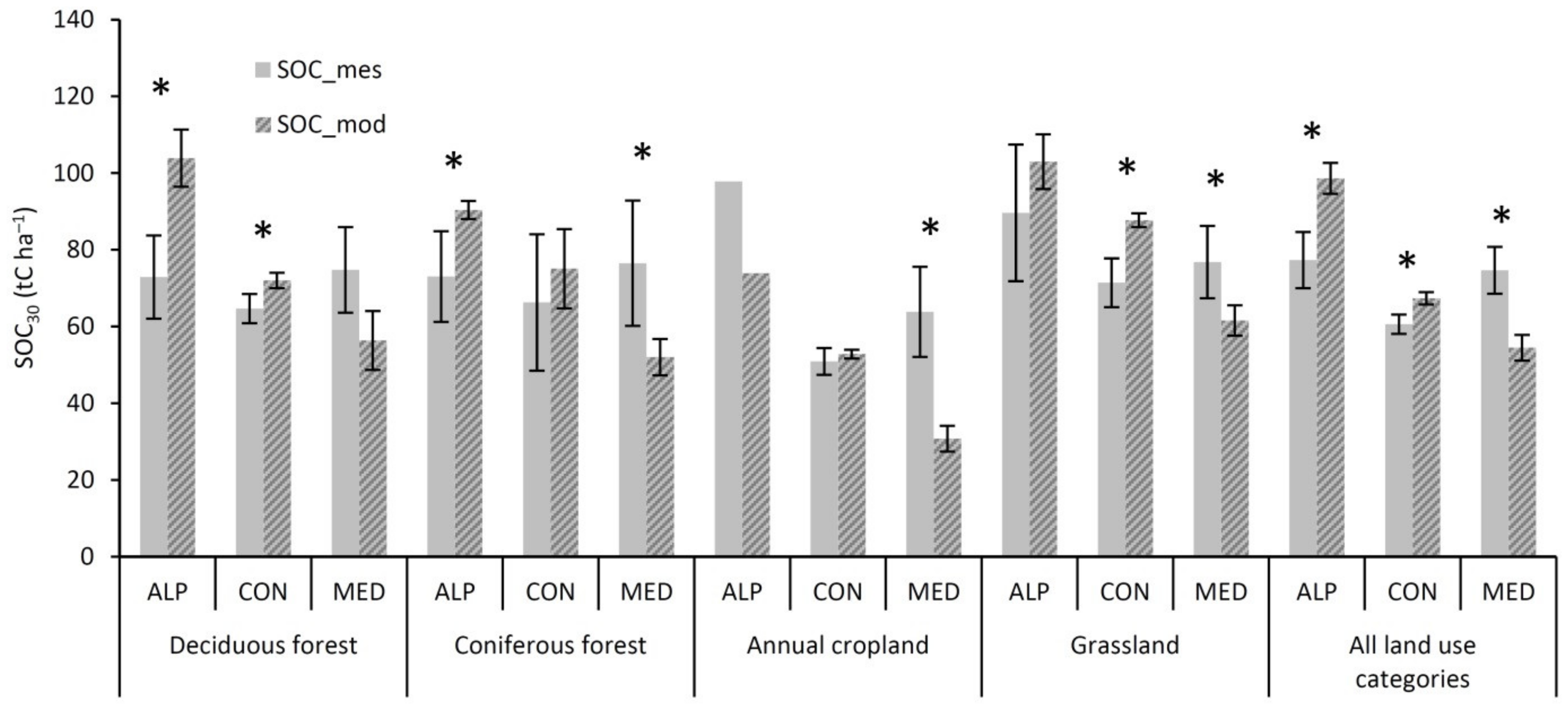
| Deciduous forest (DF) | Alpine | 33 | 72.86 ± 5.53 | 44 | 103.86 ± 3.81 | 21 |
| Continental | 178 | 64.66 ± 1.95 | 40 | 72.00 ± 1.03 | 19 | |
| Mediterranean | 30 | 74.75 ± 5.69 | 42 | 56.36 ± 3.92 | 38 | |
| Coniferous forest (CF) | Alpine | 24 | 73.02 ± 6.04 | 41 | 90.38 ± 1.21 | 7 |
| Continental | 4 | 66.26 ± 9.07 | 27 | 75.05 ± 5.27 | 14 | |
| Mediterranean | 23 | 76.49 ± 8.33 | 52 | 51.99 ± 2.43 | 22 | |
| Annual cropland (AC) | Alpine | 2 | 97.79 | 73.90 | ||
| Continental | 147 | 50.89 ± 1.77 | 42 | 52.79 ± 0.60 | 14 | |
| Mediterranean | 12 | 63.82 ± 5.99 | 33 | 30.74 ± 1.71 | 19 | |
| Grassland (GL) | Alpine | 17 | 89.60 ± 9.09 | 42 | 102.97 ± 3.65 | 15 |
| Continental | 63 | 71.40 ± 3.25 | 36 | 87.69 ± 0.92 | 8 | |
| Mediterranean | 40 | 76.78 ± 4.82 | 40 | 61.56 ± 2.02 | 21 | |
| Stratification Level | N | R2 | MAE | RMSE | NSE |
|---|---|---|---|---|---|
| Land use | 4 | 0.877 | 3.993 | 4.721 | 0.736 |
| Land use × Biogeographical region | 11 | 0.240 | 17.021 | 19.319 | −3.086 |
| Plot | 573 | 0.042 | 24.930 | 31.991 | −0.254 |
Publisher’s Note: MDPI stays neutral with regard to jurisdictional claims in published maps and institutional affiliations. |
© 2021 by the authors. Licensee MDPI, Basel, Switzerland. This article is an open access article distributed under the terms and conditions of the Creative Commons Attribution (CC BY) license (https://creativecommons.org/licenses/by/4.0/).
Share and Cite
Ostrogović Sever, M.Z.; Barcza, Z.; Hidy, D.; Kern, A.; Dimoski, D.; Miko, S.; Hasan, O.; Grahovac, B.; Marjanović, H. Evaluation of the Terrestrial Ecosystem Model Biome-BGCMuSo for Modelling Soil Organic Carbon under Different Land Uses. Land 2021, 10, 968. https://0-doi-org.brum.beds.ac.uk/10.3390/land10090968
Ostrogović Sever MZ, Barcza Z, Hidy D, Kern A, Dimoski D, Miko S, Hasan O, Grahovac B, Marjanović H. Evaluation of the Terrestrial Ecosystem Model Biome-BGCMuSo for Modelling Soil Organic Carbon under Different Land Uses. Land. 2021; 10(9):968. https://0-doi-org.brum.beds.ac.uk/10.3390/land10090968
Chicago/Turabian StyleOstrogović Sever, Maša Zorana, Zoltán Barcza, Dóra Hidy, Anikó Kern, Doroteja Dimoski, Slobodan Miko, Ozren Hasan, Branka Grahovac, and Hrvoje Marjanović. 2021. "Evaluation of the Terrestrial Ecosystem Model Biome-BGCMuSo for Modelling Soil Organic Carbon under Different Land Uses" Land 10, no. 9: 968. https://0-doi-org.brum.beds.ac.uk/10.3390/land10090968