
Historical Changes and Future Trajectories of Deforestation in the Ituri-Epulu-Aru Landscape (Democratic Republic of the Congo)

 ,
,  , ,
, ,
Abstract
:1. Introduction
2. Materials and Methods
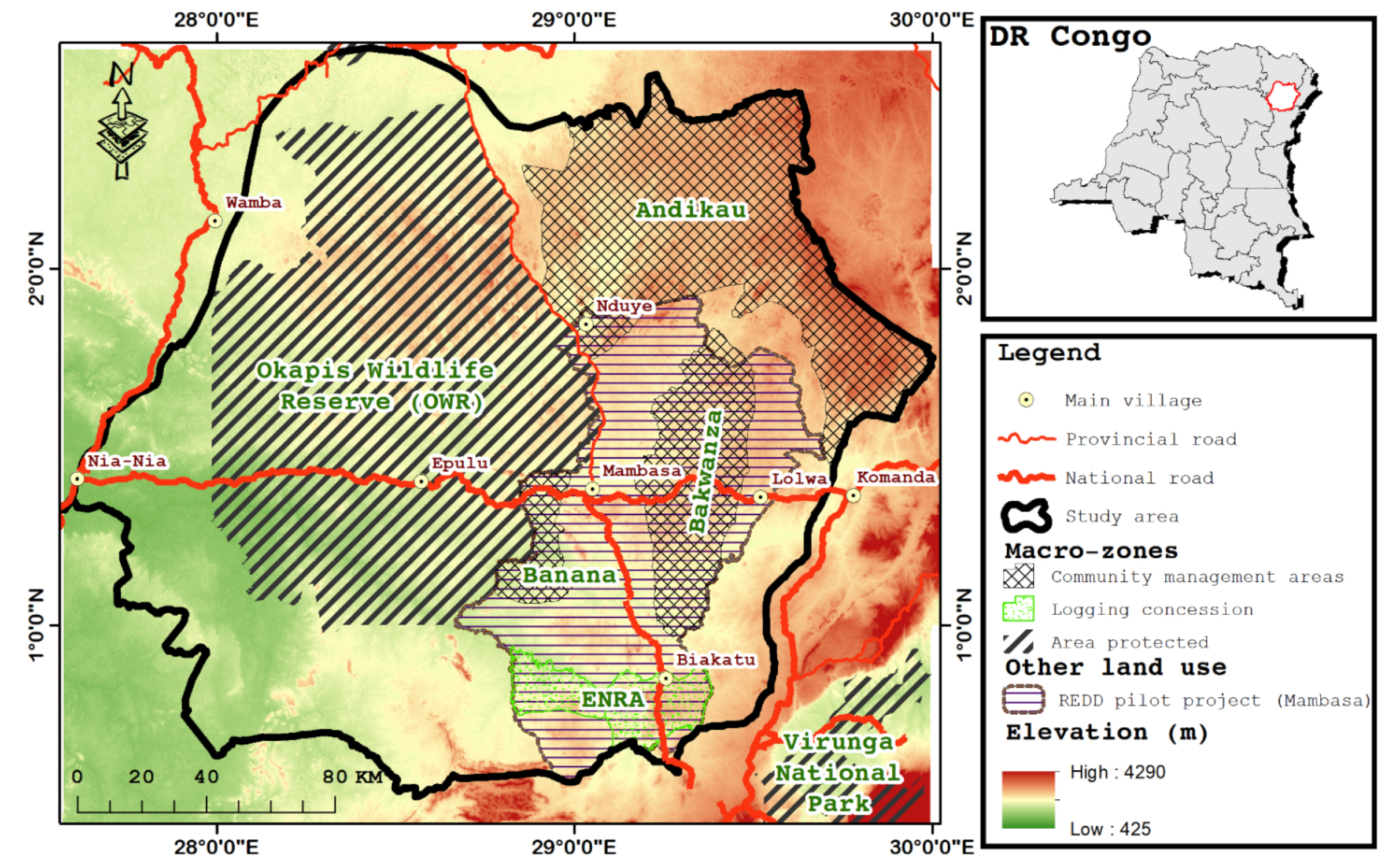
2.1. Study Area
2.2. Data Used
2.2.1. Satellite Images
2.2.2. Field Data
2.3. Methods
- Land use and land cover (LULC) classification.
- Modeling of deforestation.
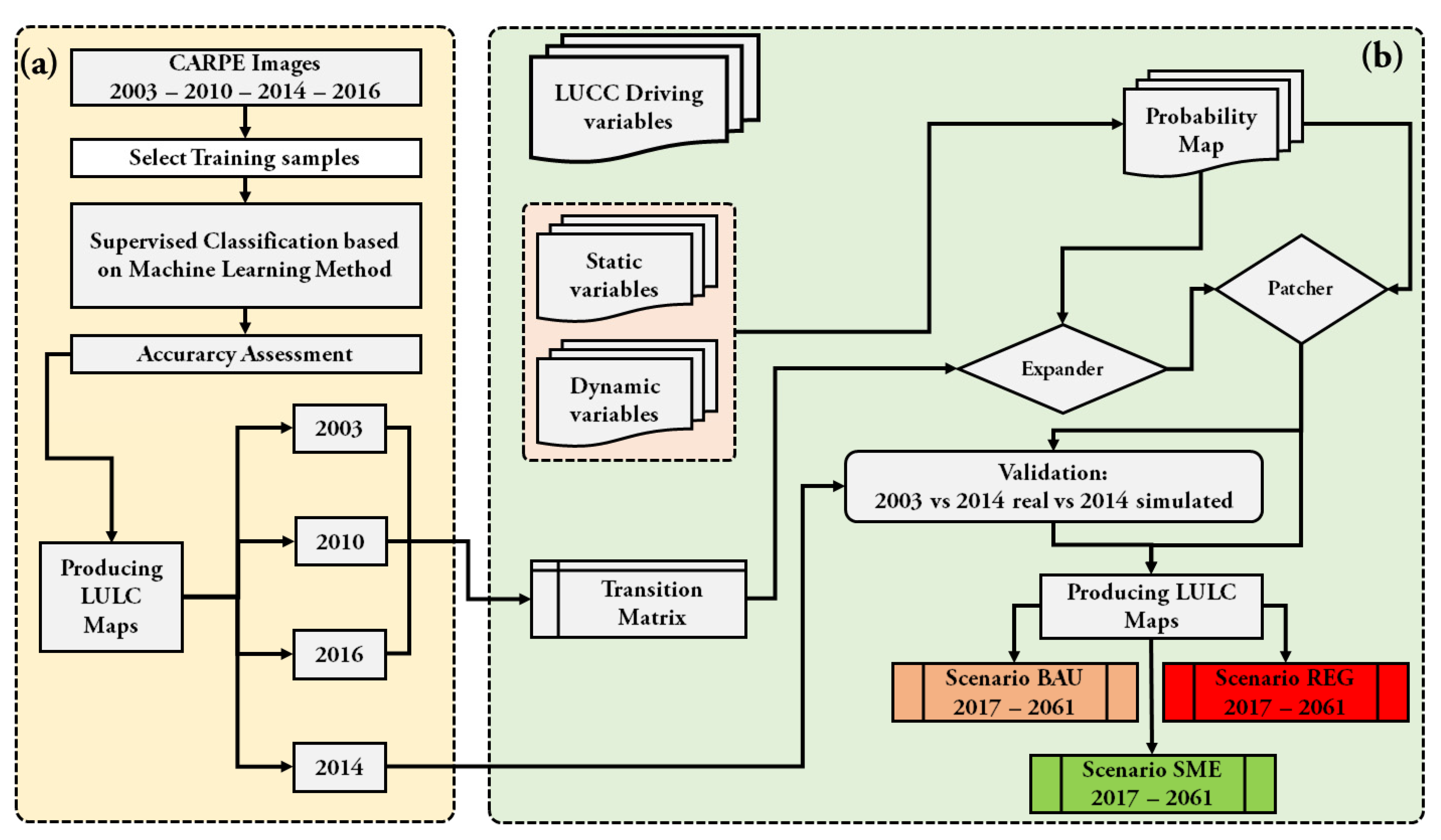
2.3.1. Land Use and Land Cover (LULC) Classification
2.3.2. Modeling of Deforestation
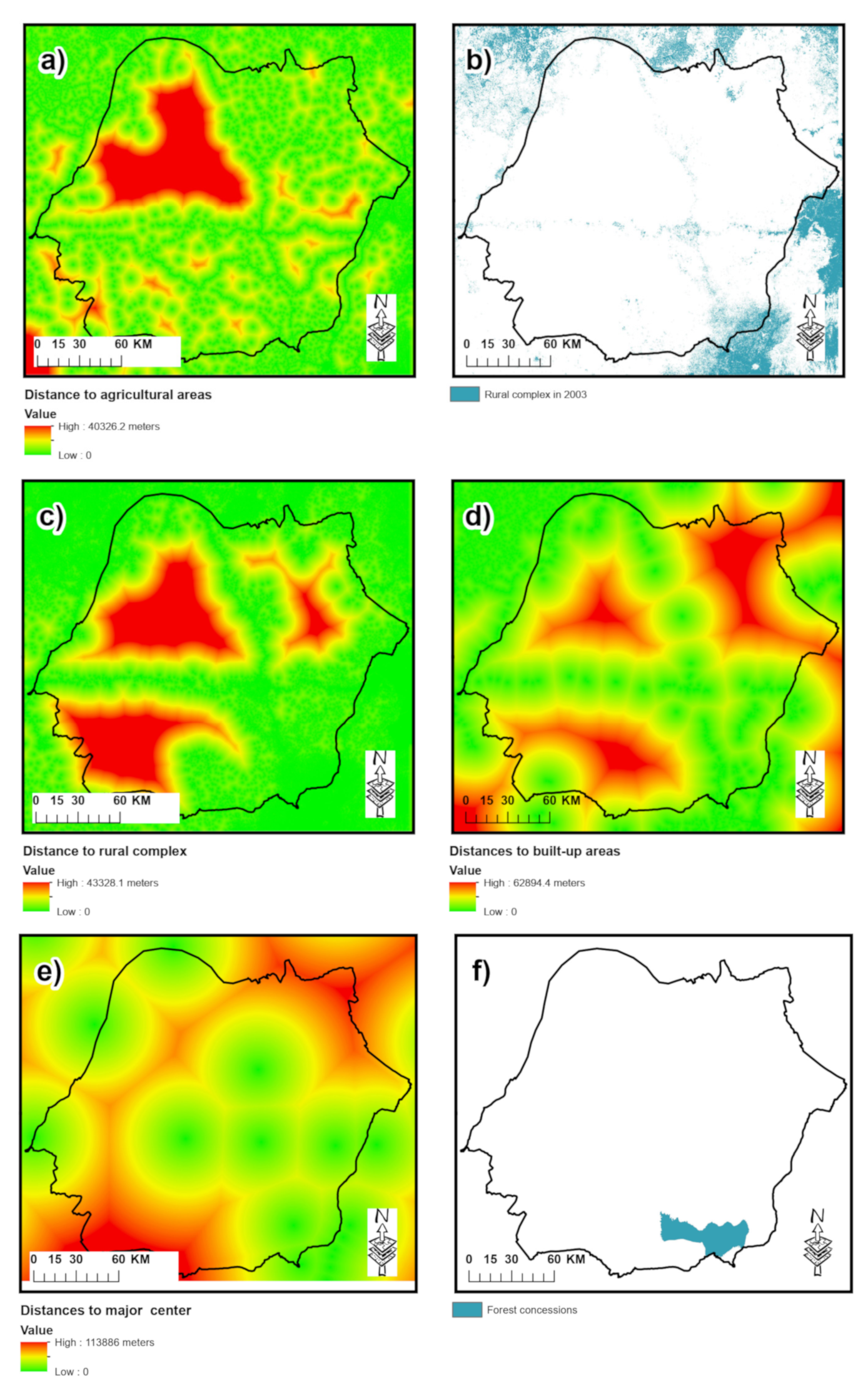
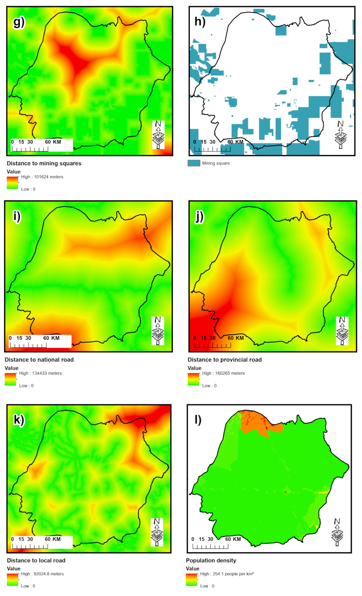
Selection of Variables
Transitions
Exploratory Analysis of the Data
Simulation of Deforestation
Validation
3. Results
3.1. Assessment of the Quality of Land Use Maps
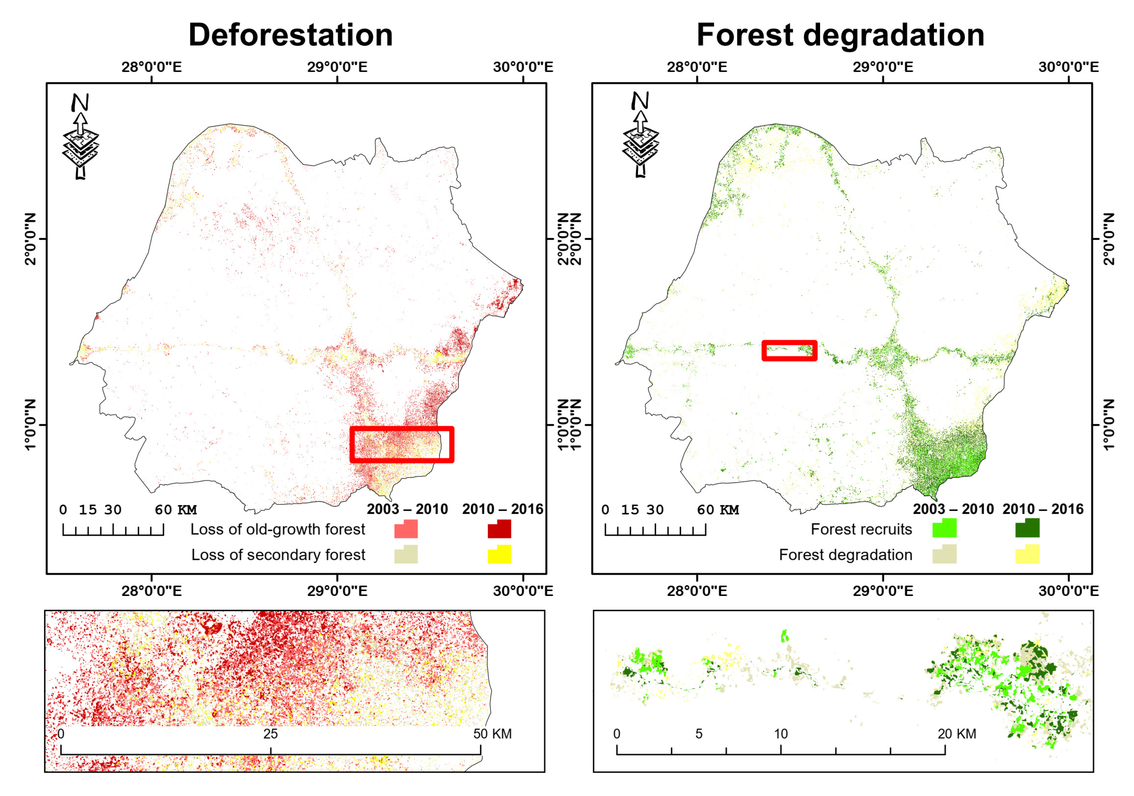
3.2. Analysis of Historical Changes of Deforestation between 2003 and 2016
3.2.1. Historical Transitions
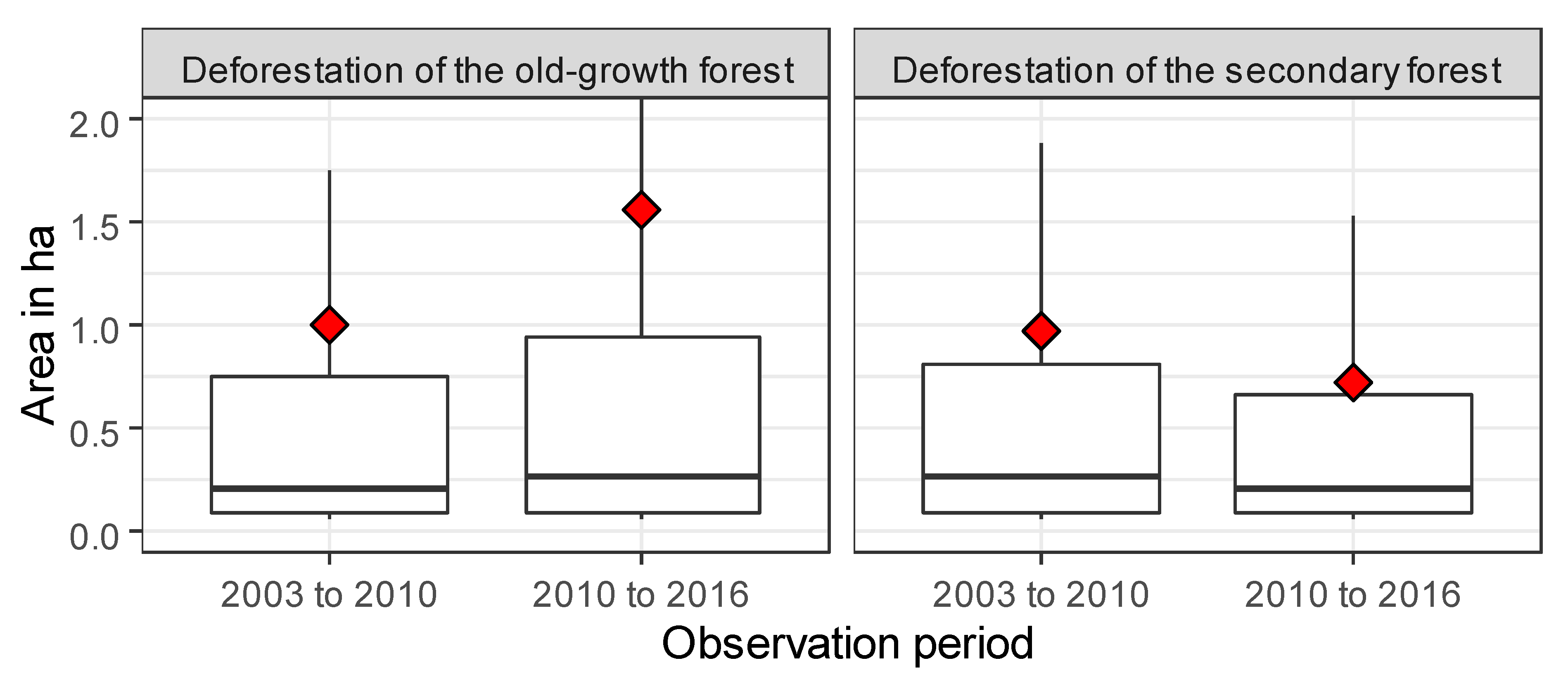
3.2.2. Deforestation Effort between 2003 and 2016
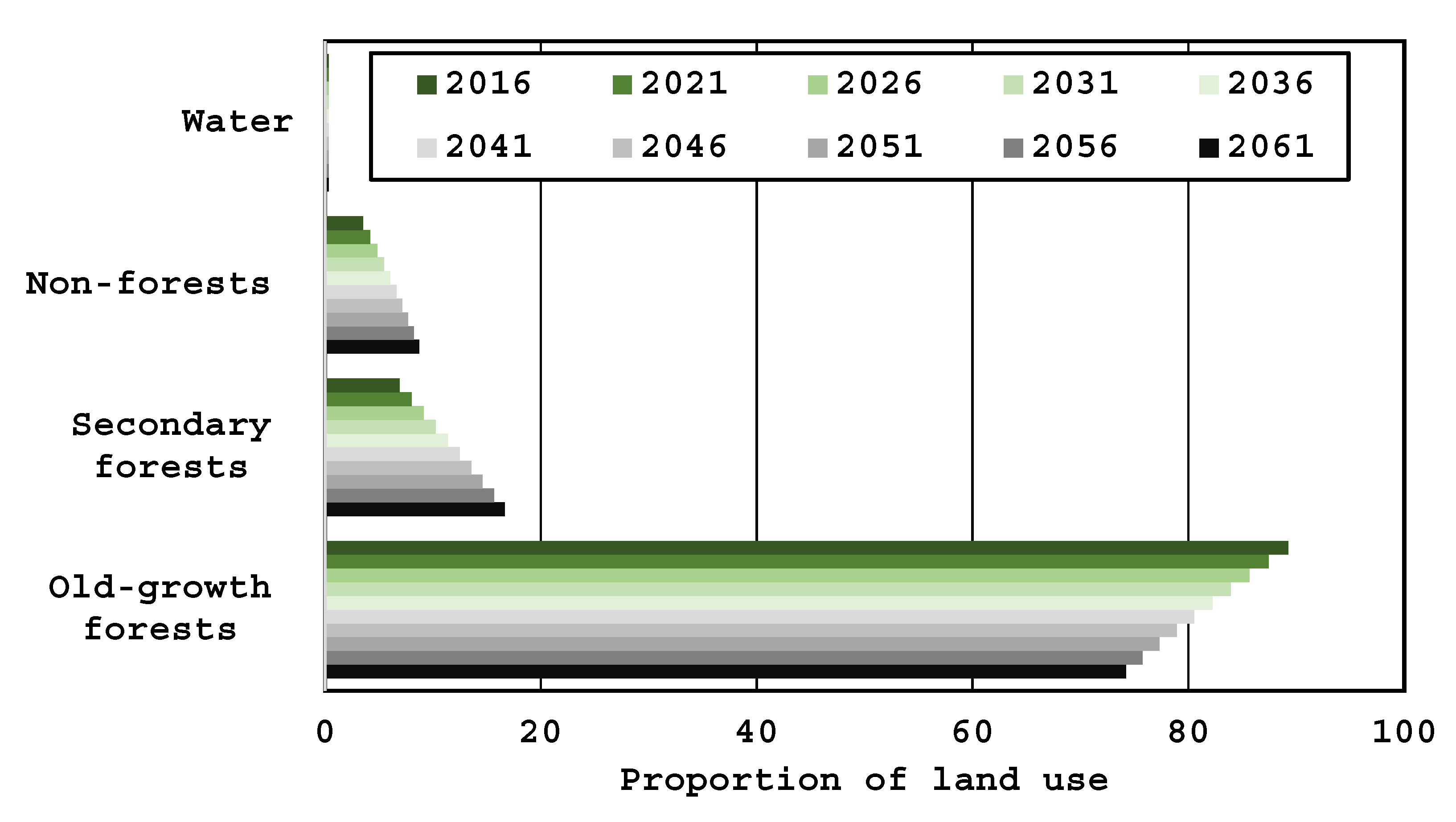
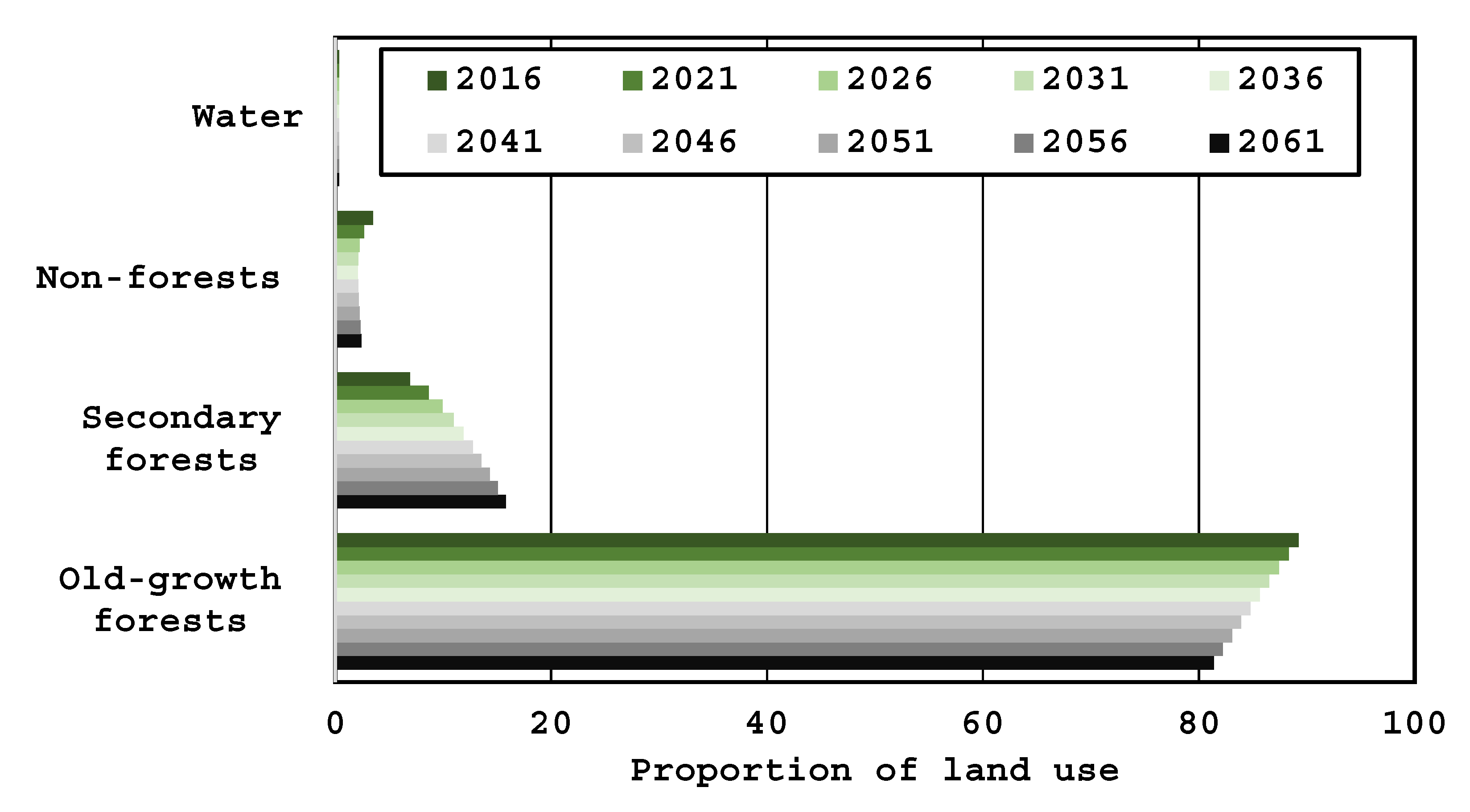
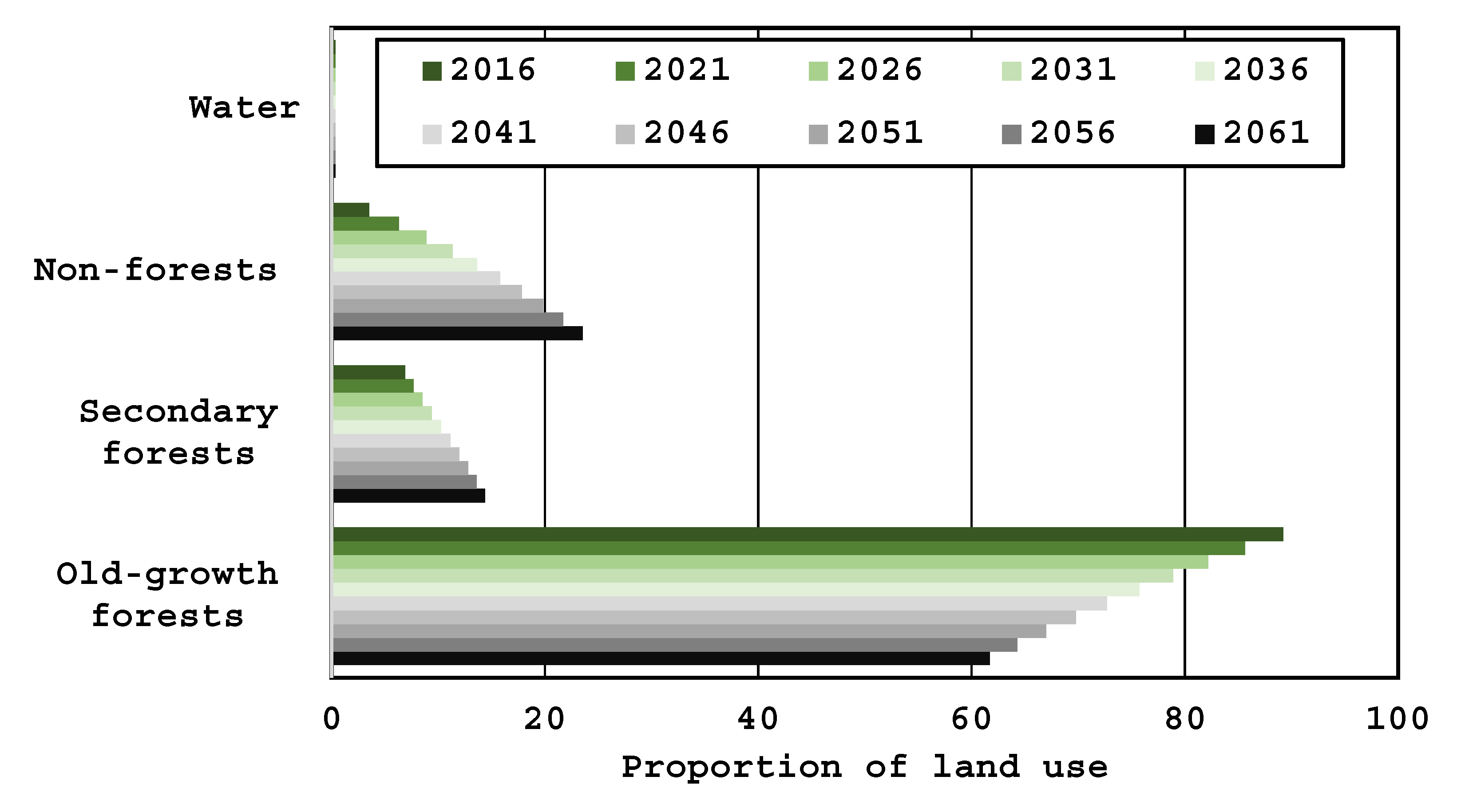
3.3. Future Trajectories of Deforestation
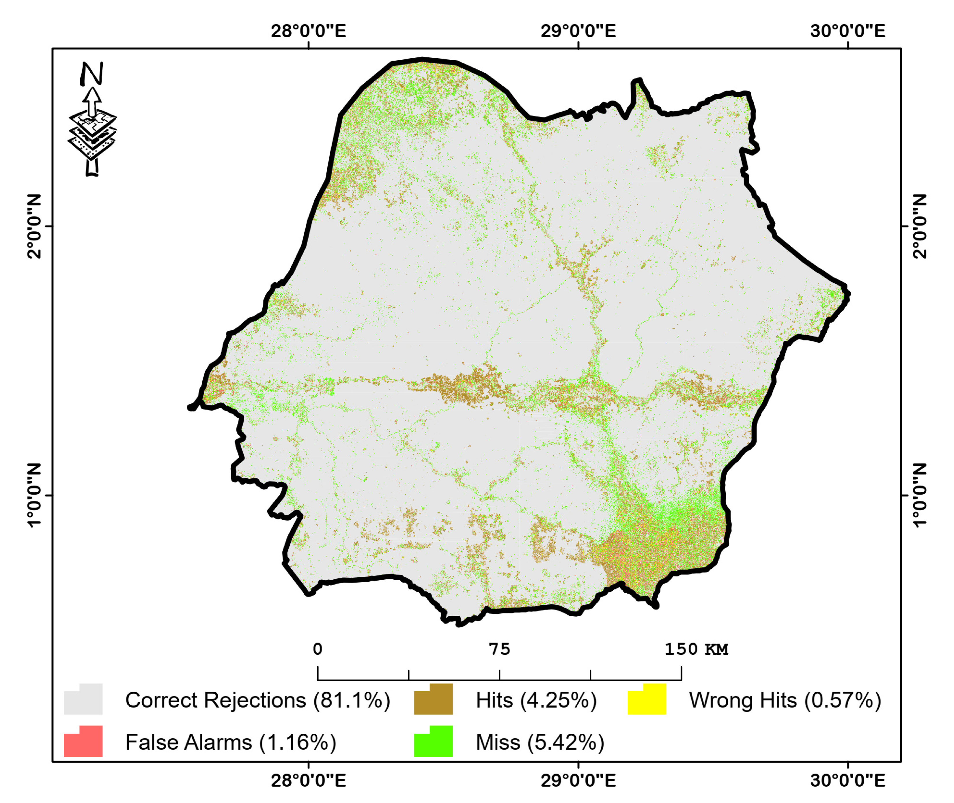
3.3.1. Validation of the Model in 2014
3.3.2. Future Trajectories of Deforestation
4. Discussion
4.1. Historical and Future Trajectories of Deforestation
4.2. Simulation of Deforestation
5. Conclusions
Author Contributions
Funding
Institutional Review Board Statement
Informed Consent Statement
Data Availability Statement
Acknowledgments
Conflicts of Interest
References
- European Commission. Joint Research Centre. Les Forêts du Bassin du Congo: État des Forêts 2010; Publications Office: Luxembourg, 2012. [Google Scholar]
- Potapov, P.V.; Turubanova, S.A.; Hansen, M.C.; Adusei, B.; Broich, M.; Altstatt, A.; Mane, L.; Justice, C.O. Quantifying forest cover loss in Democratic Republic of the Congo, 2000–2010, with Landsat ETM+ data. Remote Sens. Environ. 2012, 122, 106–116. [Google Scholar] [CrossRef]
- Bamba, I.; Barima, Y.S.S.; Bogaert, J. Influence de la densité de la population sur la structure spatiale d’un paysage forestier dans le bassin du Congo en R.D. Congo. Trop. Conserv. Sci. 2010, 3, 31–44. [Google Scholar] [CrossRef]
- Mongo, L.I.W.; Visser, M.; De Cannière, C.; Verheyen, E.; Akaibe, B.D.; Ali-Patho, J.U.; Bogaert, E.J. Anthropisation et effets de lisière: Impacts sur la diversité des rongeurs dans la réserve forestière de Masako (Kisangani, R.D. Congo). Trop. Conserv. Sci. 2012, 5, 270–283. [Google Scholar] [CrossRef] [Green Version]
- Kankonda, O.M.; Akaibe, B.D.; Sylvain, N.M.; Le Ru, B.-P. Response of maize stemborers and associated parasitoids to the spread of grasses in the rainforest zone of Kisangani, DR Congo: Effect on stemborers biological control: Response of stemborers and parasitoids to grasses spreading. Agric. For. Entomol. 2018, 20, 150–161. [Google Scholar] [CrossRef]
- Turubanova, S.; Potapov, P.V.; Tyukavina, A.; Hansen, M.C. Ongoing primary forest loss in Brazil, Democratic Republic of the Congo, and Indonesia. Environ. Res. Lett. 2018, 13, 074028. [Google Scholar] [CrossRef] [Green Version]
- Mas, J.-F.; Kolb, M.; Paegelow, M.; Camacho Olmedo, M.T.; Houet, T. Inductive pattern-based land use/cover change models: A comparison of four software packages. Environ. Model. Softw. 2014, 51, 94–111. [Google Scholar] [CrossRef] [Green Version]
- Mas, J.; Puig, P.; Palacio, J.L.; Sosa-López, A. Modelling deforestation using GIS and artificial neural networks. Environ. Model. Softw. 2004, 19, 461–471. [Google Scholar] [CrossRef]
- Pérez-Vega, A.; Mas, J.-F.; Ligmann-Zielinska, A. Comparing two approaches to land use/cover change modeling and their implications for the assessment of biodiversity loss in a deciduous tropical forest. Environ. Model. Softw. 2012, 29, 11–23. [Google Scholar] [CrossRef]
- Thierry, A.; Martin, P.; Ismaïla, T.I.; Brice, T. Modelisation des changements d’occupation des terres en region soudanienne au nord-ouest du Benin. ESJ 2018, 14, 248. [Google Scholar] [CrossRef] [Green Version]
- Defourny, P.; Delhage, C.; Kibambe, J.-P. Analyse Quantitative des Causes de la Deforestation et de la Dégradation des Forêts en République Démocratique du Congo; ULC/ELI Géomatique, Université Catholique de Louvain: Louvain-la-Neuve, Belgium, 2011; p. 104. [Google Scholar]
- Tyukavina, A.; Hansen, M.C.; Potapov, P.; Parker, D.; Okpa, C.; Stehman, S.V.; Kommareddy, I.; Turubanova, S. Congo basin forest loss dominated by increasing smallholder clearing. Sci. Adv. 2018, 4, eaat2993. [Google Scholar] [CrossRef] [Green Version]
- Hansen, M.C.; Potapov, P.V.; Moore, R.; Hancher, M.; Turubanova, S.A.; Tyukavina, A.; Thau, D.; Stehman, S.V.; Goetz, S.J.; Loveland, T.R.; et al. High-resolution global maps of 21st-century forest cover change. Science 2013, 342, 850–853. [Google Scholar] [CrossRef] [PubMed] [Green Version]
- Lusuna, M.; Kibambe, J.-P.; Makana, J.-R.; Mwinyihali, R. Evaluation par Télédétection de l’Etendue de la Couverture Forestière dans le Paysage Ituri-Epulu-Aru (2000–2014); WCS: Kinshasa, Democratic Republic of the Congo, 2014. [Google Scholar]
- PFBC. Les Forêts du Bassin du Congo: Évaluation Préliminaire; PFBC. 2005. Available online: https://carpe.umd.edu/sites/default/files/focb_aprelimassess_fr.pdf (accessed on 3 March 2021).
- UICN-PACO. Parcs et Réserves de la République Démocratique du Congo: Évaluation de l’Efficacité de la Gestion des Aires Protégées; IUCN: Gland, Switzerland, 2010. [Google Scholar]
- Forest Resources Assessment Programme. Global Forest Resources Assessment 2015; Food and Agriculture Organization of the United Nations: Rome, Italy, 2015. [Google Scholar]
- Soares-Filho, B.; Rodrigues, H.; Follador, M. A Hybrid analytical-heuristic method for calibrating land-use change models. Environ. Model. Softw. 2013, 43, 80–87. [Google Scholar] [CrossRef]
- Pontius, R.G.; Castella, J.-C.; de Nijs, T.; Duan, Z.; Fotsing, E.; Goldstein, N.; Kok, K.; Koomen, E.; Lippitt, C.D.; McConnell, W.; et al. Lessons and challenges in land change modeling derived from synthesis of cross-case comparisons. In Trends in Spatial Analysis and Modelling; Behnisch, M., Meinel, G., Eds.; Geotechnologies and the Environment; Springer International Publishing: Cham, Switzerland, 2018; Volume 19, pp. 143–164. ISBN 9783319525204. [Google Scholar]
- Verburg, P.H.; Schot, P.P.; Dijst, M.J.; Veldkamp, A. Land use change modelling: Current practice and research priorities. GeoJournal 2004, 61, 309–324. [Google Scholar] [CrossRef]
- Soares-Filho, B.S.; Coutinho Cerqueira, G.; Lopes Pennachin, C. Dinamica—A stochastic cellular automata model designed to simulate the landscape dynamics in an amazonian colonization frontier. Ecol. Model. 2002, 154, 217–235. [Google Scholar] [CrossRef]
- Brown, E.L. Ituri-Epulu-Aru. In Les Forêts du Basin du Congo—Etat des Forêts 2008; Publications Office: Luxembourg, 2010. [Google Scholar]
- Brown, E.L. Okapi faunal reserve, Ituri-Epulu-Aru landscape, Democratic Republic of the Congo. In Landscape-scale conservation in the Congo Basin: Lessons learned from the Central African Regional Program for the Environment (CARPE); UICN: Gland, Switzerland, 2010; ISBN 9782831712888. [Google Scholar]
- Masimo Kabuanga, J.; Mubenga Kankonda, O.; Horning, N.; Saqalli, M.; Maestripieri, N.; Makanzu Imwangana, F.; Mané, L. Random forest algorithm for mapping deforestation in the Ituri-Epulu-Aru landscape (Democratic Republic of the Congo). Preprints 2020, 2020120752. [Google Scholar] [CrossRef]
- Grinand, C.; Rakotomalala, F.; Gond, V.; Vaudry, R.; Bernoux, M.; Vieilledent, G. Estimating deforestation in tropical humid and dry forests in Madagascar from 2000 to 2010 using multi-date landsat satellite images and the random forests classifier. Remote Sens. Environ. 2013, 139, 68–80. [Google Scholar] [CrossRef]
- Mikwa, J.-F.; Kabuanga, J.M.; Anitambua, S.; Kahindo, M.; Nshimba, S. Analyse prospective de la déforestation estimée par télédétection dans la réserve de biosphère de Yangambi. Int. J. Innov. Sci. Res. 2016, 24, 236–256. [Google Scholar]
- Varga, O.G.; Pontius, R.G.; Singh, S.K.; Szabó, S. Intensity analysis and the figure of Merit’s components for assessment of a cellular automata—Markov simulation model. Ecol. Indic. 2019, 101, 933–942. [Google Scholar] [CrossRef]
- Pontius, R.G.; Millones, M. Death to kappa: Birth of quantity disagreement and allocation disagreement for accuracy assessment. Int. J. Remote Sens. 2011, 32, 4407–4429. [Google Scholar] [CrossRef]
- Kyale Koy, J.; Wardell, D.A.; Mikwa, J.-F.; Kabuanga, J.M.; Monga Ngonga, A.M.; Oszwald, J.; Doumenge, C. Dynamique de la déforestation dans la réserve de biosphère de Yangambi (République Démocratique Du Congo): Variabilité spatiale et temporelle au cours des 30 dernières années. Bois For. Trop. 2019, 341, 15. [Google Scholar] [CrossRef]
- Kabuanga, J.M. Analyse Diachronique Dynamique de l’Occupation du Sol à Partir de l’Imagerie Landsat TM, ETM+ et OLI; Gilman International Conservation: Epulu, Democratic Republic of the Congo, 2016; p. 36. [Google Scholar]
- Kabuanga, J.M.; Adipalina Guguya, B.; Ngenda Okito, E.; Maestripieri, N.; Saqalli, M.; Rossi, V.; Iyongo Waya Mongo, L. Suivi de l’anthropisation du paysage dans la région forestière de Babagulu, République Démocratique du Congo. Vertigo Rev. Électronique Sci. Environ. 2020. [Google Scholar] [CrossRef]
- Rodriguez-Galiano, V.F.; Chica-Olmo, M.; Abarca-Hernandez, F.; Atkinson, P.M.; Jeganathan, C. Random forest classification of mediterranean land cover using multi-seasonal imagery and multi-seasonal texture. Remote Sens. Environ. 2012, 121, 93–107. [Google Scholar] [CrossRef]
- R Core Team R: A Language and Environment for Statistical Computing; R Foundation for Statistical Computing: Vienna, Australia, 2018.
- Liaw, A.; Wiener, M. Classification and regression by RandomForest|BibSonomy. R News 2002, 2, 18–22. [Google Scholar]
- Breiman, L. Random forest. Mach. Learn. 2001, 45, 5–32. [Google Scholar] [CrossRef] [Green Version]
- Pal, M. Random forest classifier for remote sensing classification. Int. J. Remote Sens. 2005, 26, 217–222. [Google Scholar] [CrossRef]
- Gislason, P.O.; Benediktsson, J.A.; Sveinsson, J.R. Random forests for land cover classification. Pattern Recognit. Lett. 2006, 27, 294–300. [Google Scholar] [CrossRef]
- Puissant, A.; Rougier, S.; Stumpf, A. Object-oriented mapping of urban trees using random forest classifiers. Int. J. Appl. Earth Obs. Geoinf. 2014, 26, 235–245. [Google Scholar] [CrossRef]
- Strobl, C.; Boulesteix, A.-L.; Kneib, T.; Augustin, T.; Zeileis, A. Conditional variable importance for random forests. BMC Bioinform. 2008, 9, 307. [Google Scholar] [CrossRef] [Green Version]
- Van Beijma, S.; Comber, A.; Lamb, A. Random forest classification of salt marsh vegetation habitats using quad-polarimetric airborne SAR, elevation and optical RS data. Remote Sens. Environ. 2014, 149, 118–129. [Google Scholar] [CrossRef]
- Akar, Ö.; Güngör, O. Classification of multispectral images using random forest algorithm. J. Geod. Geoinf. 2012, 1, 105–112. [Google Scholar] [CrossRef] [Green Version]
- Immitzer, M.; Atzberger, C.; Koukal, T. Tree Species classification with random forest using very high spatial resolution 8-Band WorldView-2 satellite data. Remote Sens. 2012, 4, 2661–2693. [Google Scholar] [CrossRef] [Green Version]
- Teluguntla, P.; Thenkabail, P.S.; Oliphant, A.; Xiong, J.; Gumma, M.K.; Congalton, R.G.; Yadav, K.; Huete, A. A 30-m Landsat-derived cropland extent product of Australia and China using random forest machine learning algorithm on Google Earth engine cloud computing platform. ISPRS J. Photogramm. Remote Sens. 2018, 144, 325–340. [Google Scholar] [CrossRef]
- Rodrigues, H.; Soares-Filho, B. A short presentation of Dinamica EGO. In Geomatic Approaches for Modeling Land Change Scenarios; Camacho Olmedo, M.T., Paegelow, M., Mas, J.-F., Escobar, F., Eds.; Lecture Notes in Geoinformation and Cartography; Springer International Publishing: Cham, Switzerland, 2018; pp. 493–498. ISBN 9783319608013. [Google Scholar]
- Miranda-Aragón, L.; Treviño-Garza, E.J.; Jiménez-Pérez, J.; Aguirre-Calderón, O.A.; González-Tagle, M.A.; Pompa-García, M.; Aguirre-Salado, C.A. Modeling susceptibility to deforestation of remaining ecosystems in north central Mexico with logistic regression. J. For. Res. 2012, 23, 345–354. [Google Scholar] [CrossRef]
- Kabuanga, J.M. Cartographie Participative et Zonage dans la Chefferie de Mambasa; Gilman International Conservation: Epulu, Congo, 2017; p. 25. [Google Scholar]
- Institute, W.R. Atlas Forestier de la République Démocratique du Congo—Accueil. Available online: https://cod.forest-atlas.org/ (accessed on 24 June 2021).
- Linard, C.; Gilbert, M.; Snow, R.W.; Noor, A.M.; Tatem, A.J. Population distribution, settlement patterns and accessibility across Africa in 2010. PLoS ONE 2012, 7, e31743. [Google Scholar] [CrossRef] [Green Version]
- CARPE. CARPE Open Data Portal. Available online: https://carpe-worldresources.opendata.arcgis.com/ (accessed on 24 June 2021).
- Earth Resources Observation and Science (EROS). Center Shuttle Radar Topography Mission (SRTM) 1 Arc-Second Global. 2017. Available online: https://www.usgs.gov/centers/eros/science/usgs-eros-archive-digital-elevation-shuttle-radar-topography-mission-srtm-1-arc?qt-science_center_objects=0#qt-science_center_objects (accessed on 28 August 2021).
- Almeida, C.M.D.; Monteiro, A.M.V.; Câmara, G.; Soares-Filho, B.S.; Cerqueira, G.C.; Pennachin, C.L.; Batty, M. GIS and remote sensing as tools for the simulation of urban land-use change. Int. J. Remote Sens. 2005, 26, 759–774. [Google Scholar] [CrossRef] [Green Version]
- Bonham-Carter, G.F.; Merriam, D.F. Geographic Information Systems for Geoscientists: Modelling with GIS.; Elsevier Science: Amsterdam, The Netherlands, 2013; ISBN 9780080571805. [Google Scholar]
- Kamusoko, C.; Wada, Y.; Furuya, T.; Tomimura, S.; Nasu, M.; Homsysavath, K. Simulating future forest cover changes in Pakxeng district, Lao People’s Democratic Republic (PDR): Implications for sustainable forest management. Land 2013, 2, 1–19. [Google Scholar] [CrossRef] [Green Version]
- Paegelow, M.; Camacho Olmedo, M.T.; Mas, J.F. Techniques for the validation of LUCC modeling outputs. In Geomatic Approaches for Modeling Land Change Scenarios; Camacho Olmedo, M.T., Paegelow, M., Mas, J.-F., Escobar, F., Eds.; Lecture Notes in Geoinformation and Cartography; Springer International Publishing: Cham, Switzerland, 2018; pp. 53–80. ISBN 9783319608013. [Google Scholar]
- Maestripieri, N.; Paegelow, M. Validation spatiale de deux modèles de simulation: L’exemple des plantations industrielles au Chili. Cybergeo 2013. [Google Scholar] [CrossRef]
- Pontius, R.G.; Peethambaram, S.; Castella, J.-C. Comparison of three maps at multiple resolutions: A case study of land change simulation in Cho Don District, Vietnam. Ann. Assoc. Am. Geogr. 2011, 101, 45–62. [Google Scholar] [CrossRef]
- Brown, D.; Band, L.E.; Green, K.O.; Irwin, E.G.; Jain, A.; Lambin, E.F.; Pontius, R.G.; Seto, K.C.; Turner, B.L., II; Verburg, P.H. Advancing Land Change Modeling: Opportunities and Research Requirements; National Research Council (U.S.), Ed.; National Academies Press: Washington, DC, USA, 2014; ISBN 9780309288330. [Google Scholar] [CrossRef]
- Gillet, P.; Vermeulen, C.; Feintrenie, L.; Dessard, H.; Garcia, C. Quelles sont les causes de la déforestation dans le bassin du Congo? Synthèse bibliographique et études de cas. Biotechnol. Agron. Société Environ. 2016, 20, 183–194. [Google Scholar]
- Megevand, C. Dynamiques de Déforestation dans le Basin du Congo: Réconcilier la Croissance Économique et la Protection de la Forêt; The World Bank: Washington, DC, USA, 2013; ISBN 9780821398272. [Google Scholar]
- Duguma, L.A.; Atela, J.; Minang, P.A.; Ayana, A.N.; Gizachew, B.; Nzyoka, J.M.; Bernard, F. Deforestation and Forest Degradation as an Environmental Behavior: Unpacking Realities Shaping Community Actions. Land 2019, 8, 26. [Google Scholar] [CrossRef] [Green Version]
- Samie, A.; Deng, X.; Jia, S.; Chen, D. Scenario-based simulation on dynamics of land-use-land-cover change in Punjab Province, Pakistan. Sustainability 2017, 9, 1285. [Google Scholar] [CrossRef] [Green Version]
- Lajoie, G.; Hagen-Zanker, A. La Simulation de l’étalement urbain à la Réunion: Apport de l’automate Cellulaire Metronamica® pour la prospective territoriale. Cybergeo 2007. [Google Scholar] [CrossRef]
- Pontius, R.G. Component intensities to relate difference by category with difference overall. Int. J. Appl. Earth Obs. Geoinf. 2019, 77, 94–99. [Google Scholar] [CrossRef]


| Land Cover | Code | Number of Points | Description | Sources |
|---|---|---|---|---|
| Old-growth forest | Pf | 257 | Woody formation consists of a very dense cover of large trees. Old-growth forest can be semi-deciduous or evergreen, or even swampy. In all cases, the carpet of grasses is absent, and the forest has not undergone significant modification by human activities. The tree layer can reach 50 m in height. | [24,28,29] |
| Secondary forest | Sf | 302 | Woody formation corresponding to a stage of reconstitution of forest massifs which have undergone strong anthropogenic interventions, or which have evolved from wastelands. It usually has a strong dominance of moderately fast growing semi-heliophilic species. The tree layer generally reaches 35 m in height | [6,24,29,30,31] |
| Non-Forest | NF | 315 | Non-forest plant formation including wasteland, shrub savannah, land cultivated on an itinerant or intensive basis, as well as recent fallows. This class also includes areas occupied by buildings, dwellings and other high-density constructions as well as areas without vegetation with bare soil, rocky outcrops or even sandy beaches along rivers. This class is represented by the major roads and their right-of-way | [24,28,30,31,32] |
| Water | Ww | 76 | This class includes all bodies of water, including the Ituri River and Epulu | [13,24,28,30] |
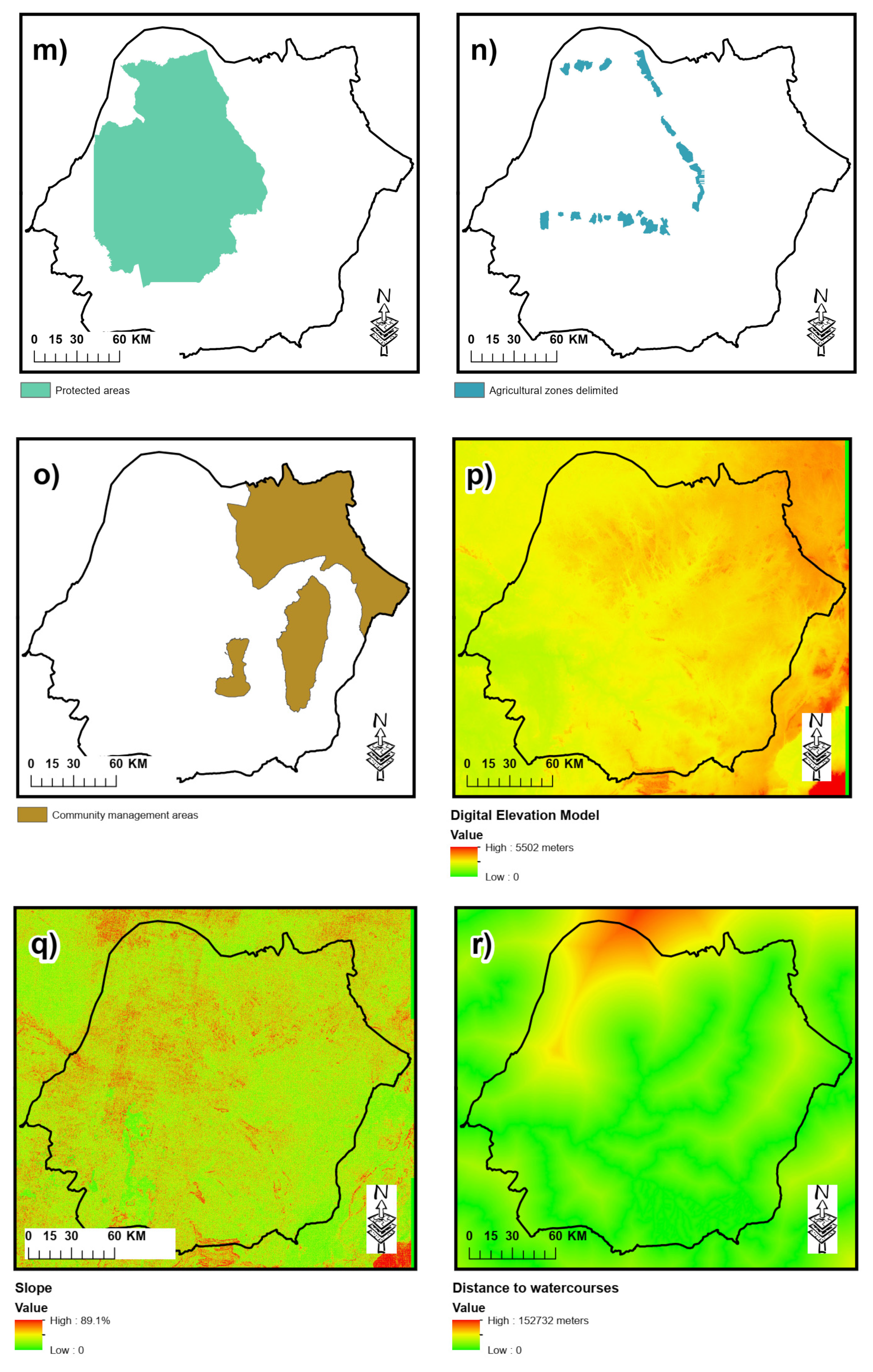
| Category | Variable Retained | Code | Sources |
|---|---|---|---|
| Agriculture | Distance to agricultural areas | d_agri | Spatial analysis [24] |
| Rural complex | Comp | [24] | |
| Distance to rural complex | d_comp | Spatial analysis [24] | |
| Economic factors | Distances to built-up areas | d_abat | Spatial analysis [24] |
| Distances to major center | d_gcent | Spatial analysis [24] | |
| Forest concessions | Ccf | [47] | |
| Mining square | Mining | [47] | |
| Distance to mining squares | d_mining | Spatial analysis [47] | |
| Transport | Distance to national road | d_road1 | Spatial analysis [47] |
| Distance to provincial road | d_road2 | Spatial analysis [47] | |
| Distance to local road | d_road3 | Spatial analysis [47] | |
| Demographic factors | Population density | Dens | [48] |
| Sociopolitical factors | Protected areas | Ap | [49] |
| Agricultural zones delimited | Areaagr | [49] | |
| community management | Areamngt | [49] | |
| Biophysical factors | Elevation | Dme | [50] |
| Slope | Slope | Spatial analysis [50] | |
| Distance to watercourses | d_w | Spatial analysis [13,24,50] | |
| Distances to non-forests | d_nf | Spatial analysis [24,30,46] | |
| Distance to degraded forest | d_fd | Spatial analysis [24] |
| Comparison of Three Maps | ||||
|---|---|---|---|---|
| 2003 | 2014 | 2014si | Components | |
| 1 | 1 | 1 | Reference persistence simulated correctly as persistence | Correct rejections |
| 2 | 2 | 2 | ||
| 3 | 3 | 3 | ||
| 4 | 4 | 4 | ||
| 1 | 2 | 1 | Reference change simulated incorrectly as persistence | Misses |
| 1 | 3 | 1 | ||
| 1 | 4 | 1 | ||
| 2 | 1 | 2 | ||
| 2 | 3 | 2 | ||
| 2 | 4 | 2 | ||
| 3 | 1 | 3 | ||
| 3 | 2 | 3 | ||
| 3 | 4 | 3 | ||
| 4 | 1 | 4 | ||
| 4 | 2 | 4 | ||
| 4 | 3 | 4 | ||
| 1 | 1 | 2 | Reference persistence simulated incorrectly as change | False Alarms |
| 1 | 1 | 3 | ||
| 1 | 1 | 4 | ||
| 2 | 2 | 1 | ||
| 2 | 2 | 3 | ||
| 2 | 2 | 4 | ||
| 3 | 3 | 1 | ||
| 3 | 3 | 2 | ||
| 3 | 3 | 4 | ||
| 4 | 4 | 1 | ||
| 4 | 4 | 2 | ||
| 4 | 4 | 3 | ||
| 1 | 2 | 2 | Reference change simulated correctly as change | Hits |
| 1 | 3 | 3 | ||
| 1 | 4 | 4 | ||
| 2 | 1 | 1 | ||
| 2 | 3 | 3 | ||
| 2 | 4 | 4 | ||
| 3 | 1 | 1 | ||
| 3 | 2 | 2 | ||
| 3 | 4 | 4 | ||
| 4 | 1 | 1 | ||
| 4 | 2 | 2 | ||
| 4 | 3 | 3 | ||
| 1 | 2 | 3 | Reference change simulated incorrectly as change to the wrong gaining category | Wrong Hits |
| 1 | 2 | 4 | ||
| 1 | 3 | 2 | ||
| 1 | 3 | 4 | ||
| 1 | 4 | 2 | ||
| 1 | 4 | 3 | ||
| 2 | 1 | 3 | ||
| 2 | 1 | 4 | ||
| 2 | 3 | 1 | ||
| 2 | 3 | 4 | ||
| 2 | 4 | 1 | ||
| 2 | 4 | 3 | ||
| 3 | 1 | 2 | ||
| 3 | 1 | 4 | ||
| 3 | 2 | 1 | ||
| 3 | 2 | 4 | ||
| 3 | 4 | 1 | ||
| 3 | 4 | 2 | ||
| 4 | 1 | 2 | ||
| 4 | 1 | 3 | ||
| 4 | 2 | 1 | ||
| 4 | 2 | 3 | ||
| 4 | 3 | 1 | ||
| 4 | 3 | 2 | ||
| Accuracy | Land Use | 2003 | 2010 | 2014 | 2016 |
|---|---|---|---|---|---|
| User | Pf | 0.91 | 0.93 | 0.89 | 0.98 |
| Sf | 0.78 | 0.82 | 0.79 | 0.77 | |
| Nf | 0.81 | 0.82 | 0.79 | 0.85 | |
| Ww | 0.92 | 0.94 | 0.91 | 0.90 | |
| Producer | Pf | 0.89 | 0.90 | 0.86 | 0.94 |
| Sf | 0.77 | 0.79 | 0.76 | 0.81 | |
| Nf | 0.79 | 0.80 | 0.78 | 0.82 | |
| Ww | 0.90 | 0.92 | 0.89 | 0.95 | |
| Over all | 0.91 | 0.93 | 0.93 | 0.97 | |
| Forest Type | Forest Areas | Deforested Areas | ||||||||
|---|---|---|---|---|---|---|---|---|---|---|
| 2003 | 2010 | 2016 | 2003–2010 | 2010–2016 | ||||||
| Ha | % | Ha | % | Ha | % | DA | Td | DA | Td | |
| Pf | 3,801,767 | 91.75 | 3,751,719 | 91.73 | 3,643,399 | 89.28 | 50,048 | 0.19 | 108,319 | 0.42 |
| Sf | 178,472 | 5.83 | 213,538 | 5.28 | 284,351 | 6.91 | −35,065 | −2.56 | −70,813 | −4.09 |
| Total | 3,980,240 | 97.58 | 3,965,257 | 91.73 | 3,927,751 | 96.19 | 14,983 | 0.05 | 37,505 | 0.14 |
| 2003–2016 | Land Use in 2016 | Total 2003 | ||||
|---|---|---|---|---|---|---|
| Pf | Sf | Nf | Ww | |||
| Land use in 2003 | Pf | 87.66 | 2.18 | 1.90 | 0.00 | 91.75 |
| Sf | 1.61 | 3.59 | 0.62 | 0.00 | 5.83 | |
| Nf | 0.00 | 1.14 | 0.97 | 0.00 | 2.12 | |
| Ww | 0.00 | 0.00 | 0.00 | 0.31 | 0.31 | |
| Total 2016 | 89.28 | 6.91 | 3.50 | 0.31 | 100 | |
| Observed–Simulated | Simulated Land Use in 2014 | Total Observed | ||||
|---|---|---|---|---|---|---|
| Pf | Sf | Nf | Ww | |||
| Observed land use in 2014 | Pf | 84.87 | 3.64 | 1.68 | 0.00 | 90.20 |
| Sf | 1.55 | 3.54 | 1.06 | 0.00 | 6.16 | |
| Nf | 0.99 | 0.99 | 1.37 | 0.00 | 3.36 | |
| Ww | 0.00 | 0.00 | 0.00 | 0.29 | 0.28 | |
| Total simulated | 87.42 | 8.17 | 4.11 | 0.29 | 100 | |
| 2016–2061 | Land Use in 2061 | Total 2016 | ||||
|---|---|---|---|---|---|---|
| Pf | Sf | Nf | Ww | |||
| Land use in 2016 | Pf | 80.11 | 7.86 | 1.30 | 0.00 | 89.28 |
| Sf | 0.21 | 5.95 | 0.75 | 0.00 | 6.91 | |
| Nf | 0.12 | 2.73 | 0.66 | 0.00 | 3.50 | |
| Ww | 0.00 | 0.00 | 0.00 | 0.31 | 0.31 | |
| Total 2061 | 80.44 | 16.54 | 2.71 | 0.31 | 100 | |
| 2016–2061 | Land Use in 2061 | Total 2016 | ||||
|---|---|---|---|---|---|---|
| Pf | Sf | Nf | Ww | |||
| Land use in 2016 | Pf | 59.13 | 12.62 | 17.52 | 0.00 | 89.28 |
| Sf | 0.11 | 1.92 | 4.87 | 0.00 | 6.91 | |
| Nf | 0.07 | 0.58 | 2.86 | 0.00 | 3.50 | |
| Ww | 0.00 | 0.00 | 0.00 | 0.31 | 0.31 | |
| Total 2061 | 59.31 | 15.13 | 25.25 | 0.31 | 100 | |
Publisher’s Note: MDPI stays neutral with regard to jurisdictional claims in published maps and institutional affiliations. |
© 2021 by the authors. Licensee MDPI, Basel, Switzerland. This article is an open access article distributed under the terms and conditions of the Creative Commons Attribution (CC BY) license (https://creativecommons.org/licenses/by/4.0/).
Share and Cite
Kabuanga, J.M.; Kankonda, O.M.; Saqalli, M.; Maestripieri, N.; Bilintoh, T.M.; Mweru, J.-P.M.; Liama, A.B.; Nishuli, R.; Mané, L. Historical Changes and Future Trajectories of Deforestation in the Ituri-Epulu-Aru Landscape (Democratic Republic of the Congo). Land 2021, 10, 1042. https://0-doi-org.brum.beds.ac.uk/10.3390/land10101042
Kabuanga JM, Kankonda OM, Saqalli M, Maestripieri N, Bilintoh TM, Mweru J-PM, Liama AB, Nishuli R, Mané L. Historical Changes and Future Trajectories of Deforestation in the Ituri-Epulu-Aru Landscape (Democratic Republic of the Congo). Land. 2021; 10(10):1042. https://0-doi-org.brum.beds.ac.uk/10.3390/land10101042
Chicago/Turabian StyleKabuanga, Joël Masimo, Onésime Mubenga Kankonda, Mehdi Saqalli, Nicolas Maestripieri, Thomas Mumuni Bilintoh, Jean-Pierre Mate Mweru, Aimé Balimbaki Liama, Radar Nishuli, and Landing Mané. 2021. "Historical Changes and Future Trajectories of Deforestation in the Ituri-Epulu-Aru Landscape (Democratic Republic of the Congo)" Land 10, no. 10: 1042. https://0-doi-org.brum.beds.ac.uk/10.3390/land10101042