
Sediment Yield in Dam-Controlled Watersheds in the Pisha Sandstone Region on the Northern Loess Plateau, China


 and
and
Abstract
:1. Introduction
2. Study Area
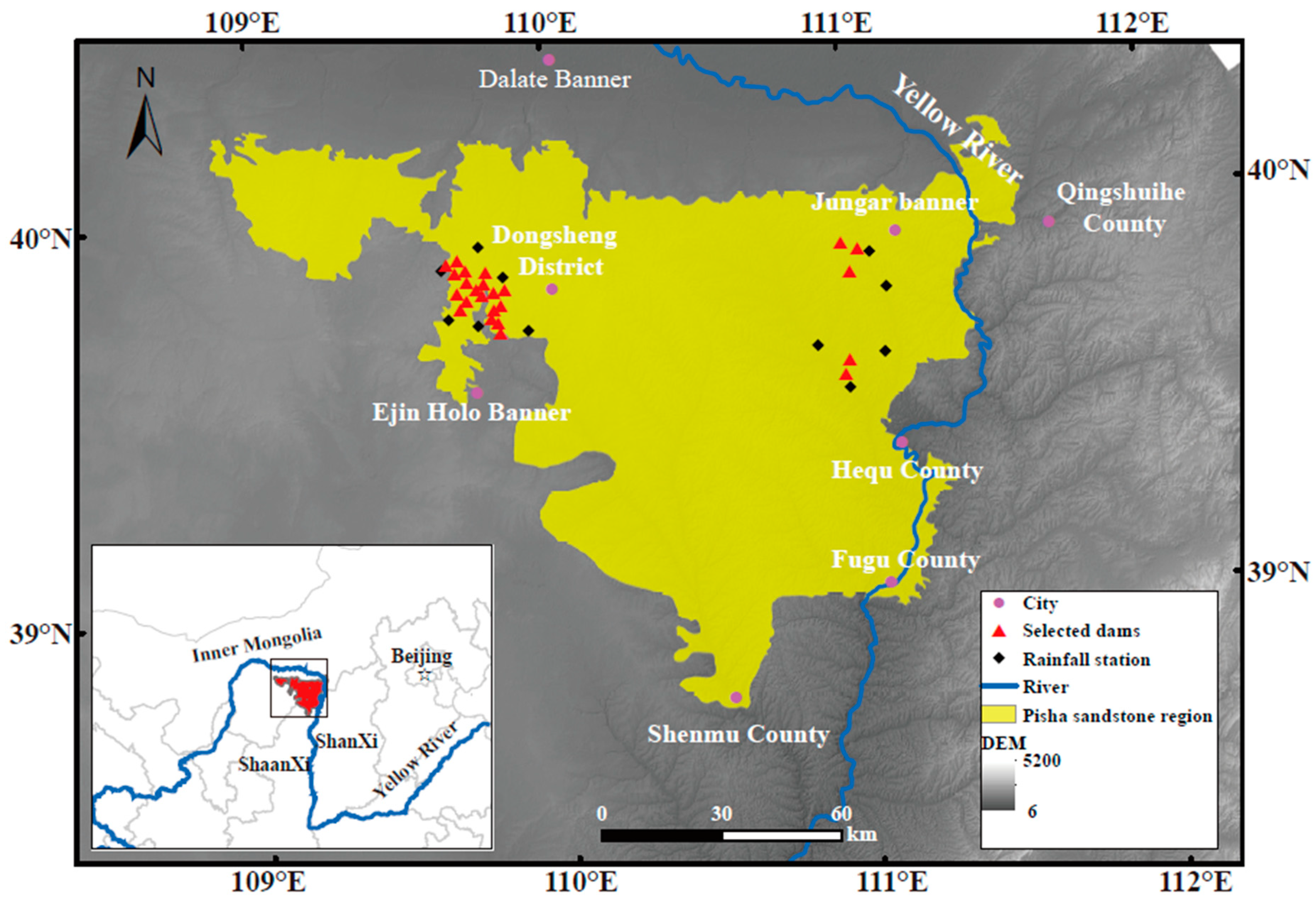
2.1. Study Area
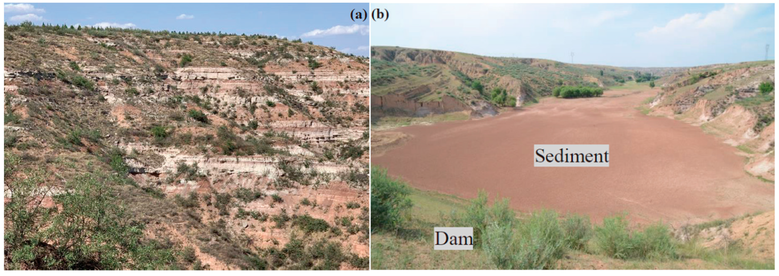
2.2. Selection of Watersheds
3. Material and Methods
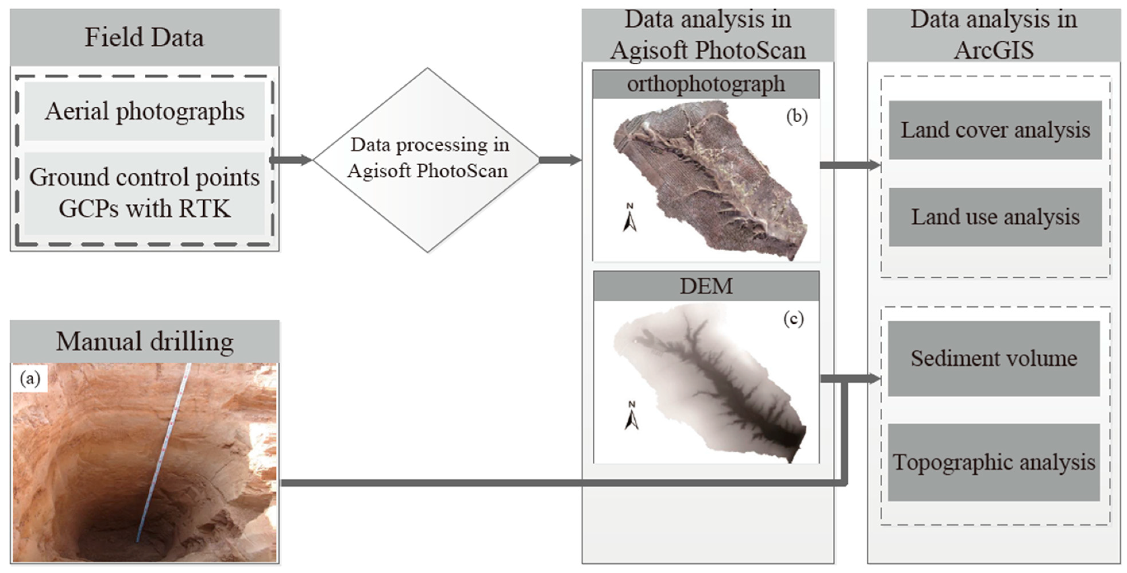
3.1. Sediment Yield Estimations for Small Watersheds
3.2. The SEDD Model
3.3. Statistical Analysis
4. Results
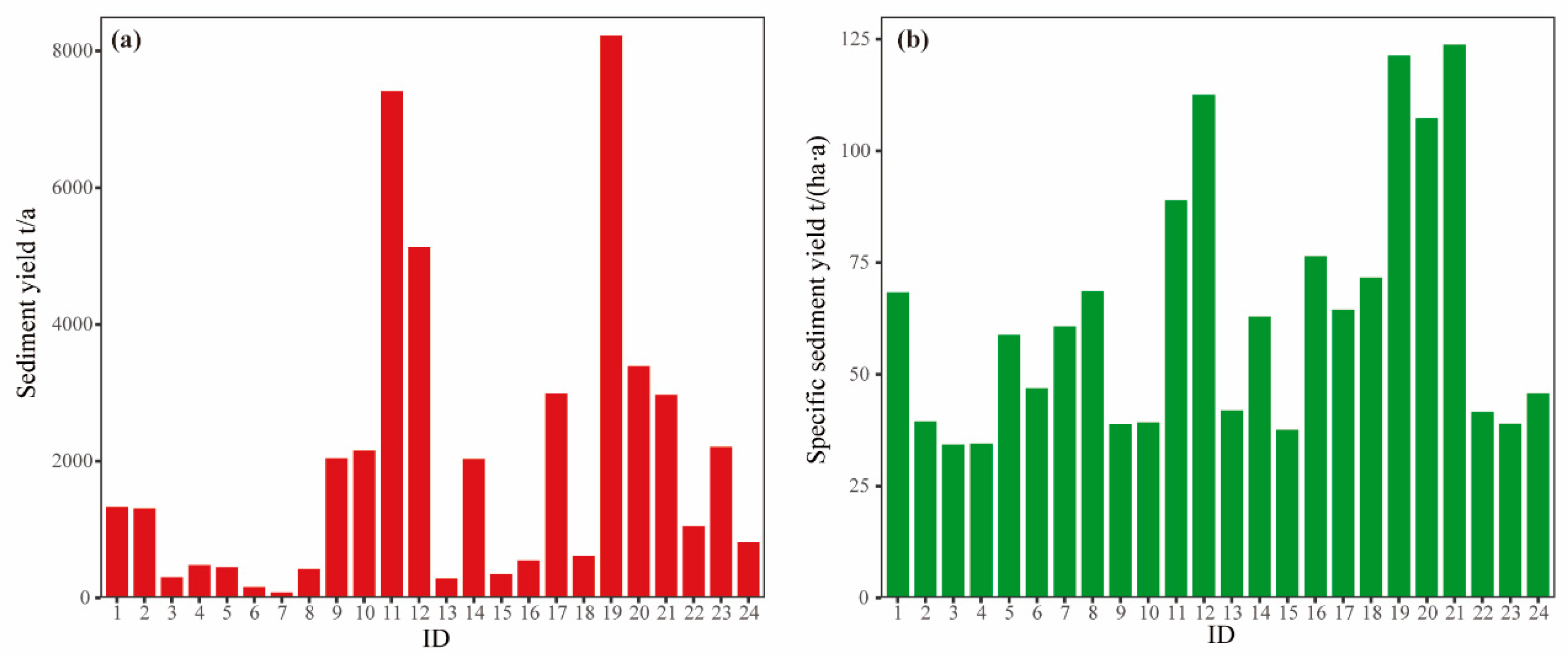
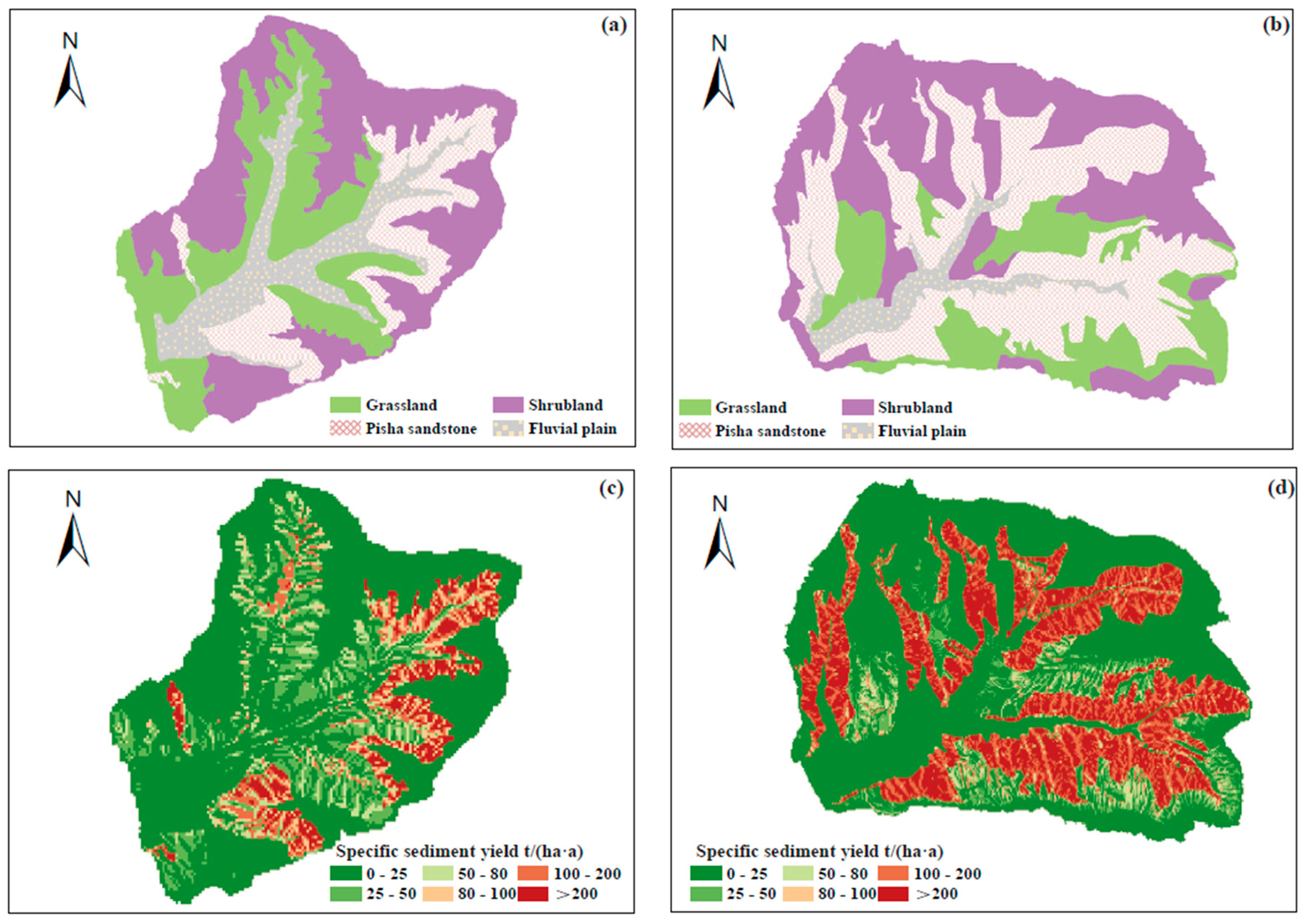
4.1. Sediment Yield Estimation
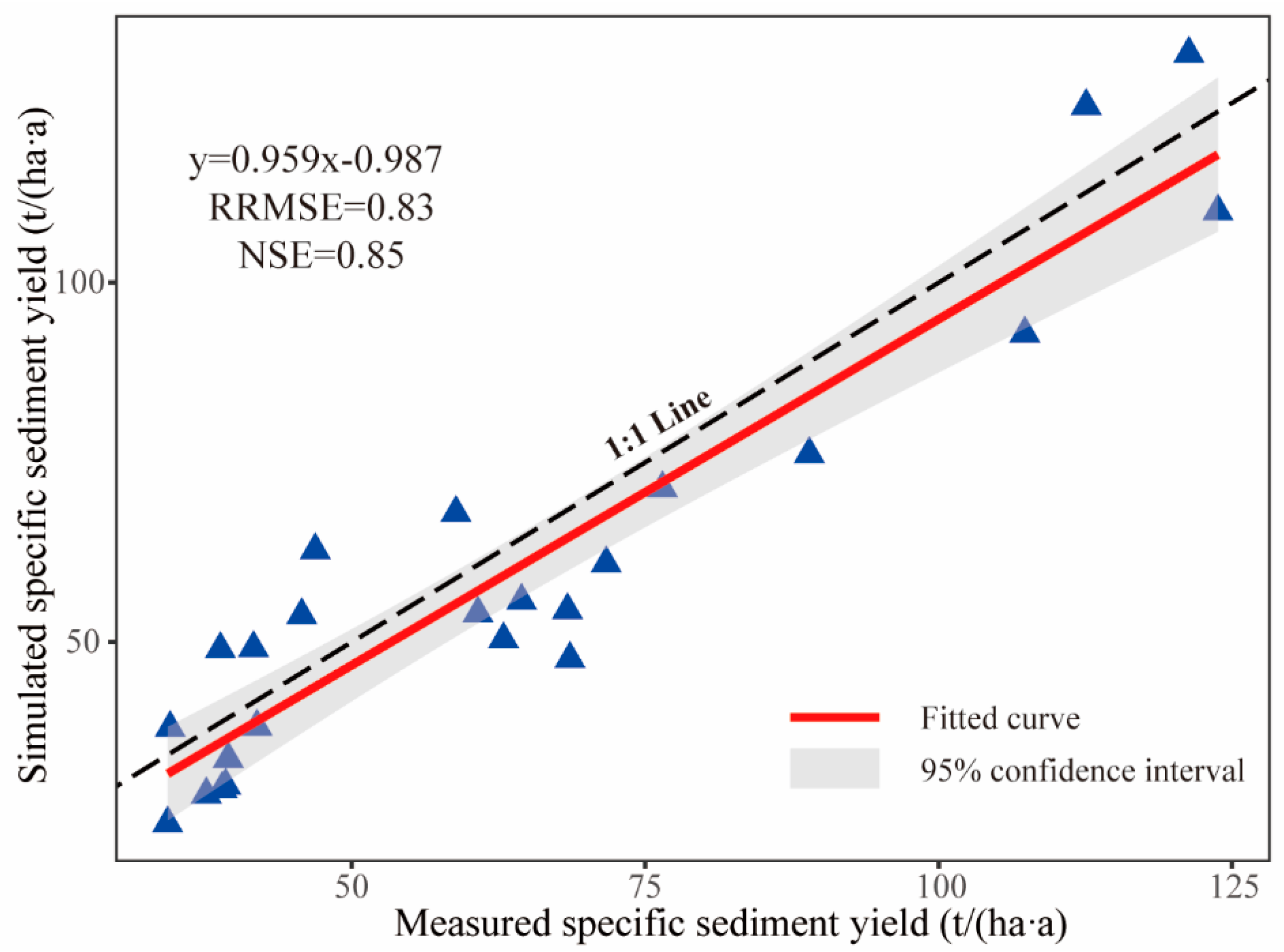
4.2. Model Calibration and Validation
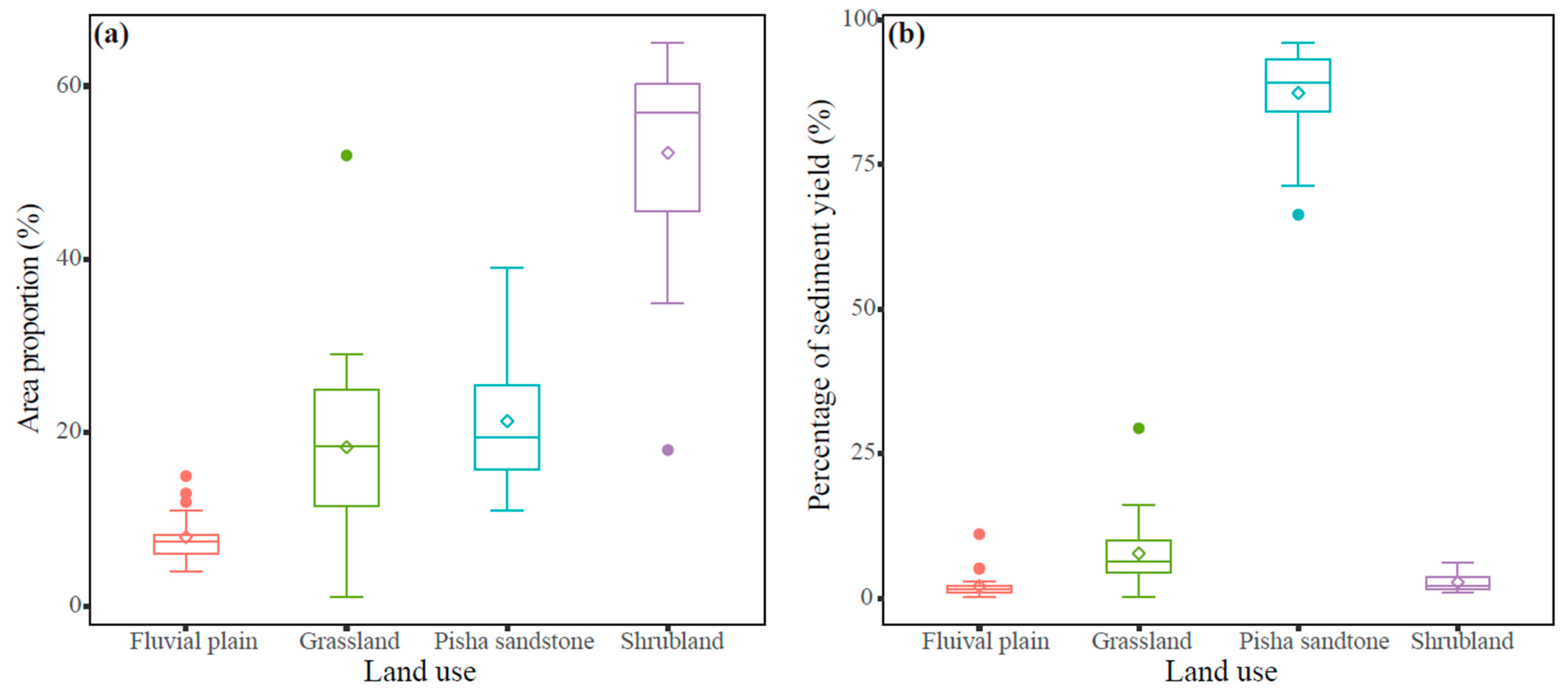
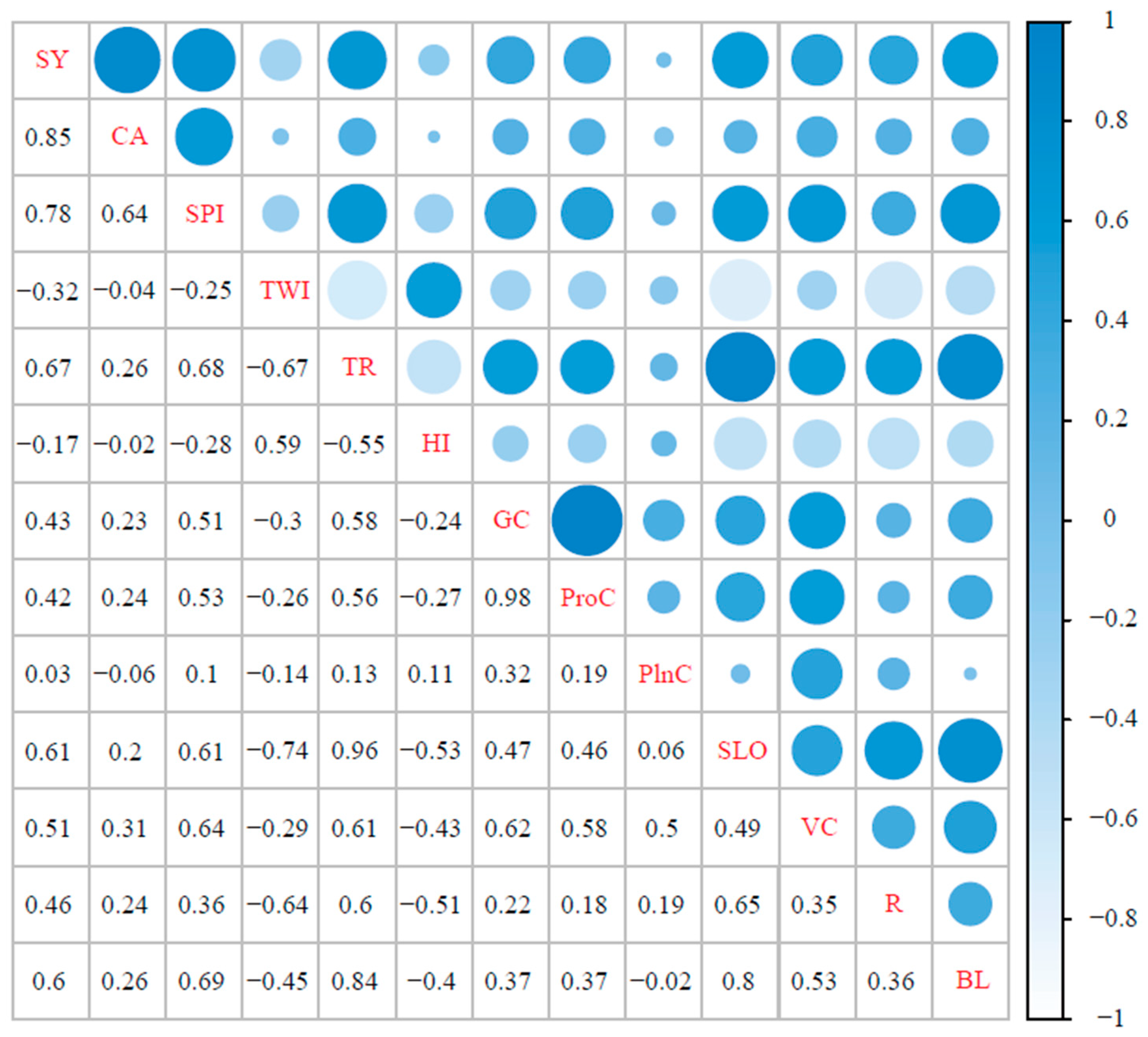
4.3. Relationships between Sediment Yield and Environment Variable
5. Discussion
5.1. Estimation of Sediment Yield in The Small Watersheds
5.2. Model Performance
5.3. The Key Factors Affecting Sediment Yield
6. Conclusions
Author Contributions
Funding
Institutional Review Board Statement
Informed Consent Statement
Data Availability Statement
Acknowledgments
Conflicts of Interest
References
- Feng, X.; Wang, Y.; Chen, L.; Fu, B.; Bai, G. Modeling soil erosion and its response to land-use change in hilly catchments of the Chinese Loess Plateau. Geomorphology 2010, 118, 239–248. [Google Scholar] [CrossRef]
- Fu, B.; Liu, Y.; Lue, Y.; He, C.; Zeng, Y.; Wu, B. Assessing the soil erosion control service of ecosystems change in the Loess Plateau of China. Ecol. Complex. 2011, 8, 284–293. [Google Scholar] [CrossRef]
- Pimentel, D. Soil Erosion: A Food and Environmental Threat. Environ. Dev. Sustain. 2006, 8, 119–137. [Google Scholar] [CrossRef]
- Tian, P.; An, Z.; Zhao, G.; Gao, P.; Li, P.; Sun, W.; Mu, X. Assessing sediment yield and sources using fingerprinting method in a representative catchment of the Loess Plateau, China. Environ. Earth Sci. 2019, 78, 261–272. [Google Scholar] [CrossRef]
- Romero-Díaz, A.; Marín-Sanleandro, P.; Ortiz-Silla, R. Loss of soil fertility estimated from sediment trapped in check dams. South-eastern Spain. Catena 2012, 99, 42–53. [Google Scholar] [CrossRef]
- Polyakov, V.; Nichols, M.; Mcclaran, M.; Nearing, M. Effect of check dams on runoff, sediment yield, and retention on small semiarid watersheds. J. Soil Water Conserv. 2014, 69, 414–421. [Google Scholar] [CrossRef] [Green Version]
- Abbasi, N.; Xu, X.; Lucas-Borja, M.; Dang, W.; Liu, B. The use of check dams in watershed management projects: Examples from around the world. Sci. Total Environ. 2019, 676, 683–691. [Google Scholar] [CrossRef]
- Shen, W.; Wang, D.; Qu, H.; Li, T. The effect of check dams on the dynamic and bed entrainment processes of debris flows. Landslides 2019, 16, 2201–2217. [Google Scholar] [CrossRef]
- Huang, J.; Hinokidani, O.; Yasuda, H.; Ojha, C.; Kajikawa, Y.; Li, S. Effects of the Check Dam System on Water Redistribution in the Chinese Loess Plateau. J. Hydrol. Eng. 2013, 18, 929–940. [Google Scholar] [CrossRef]
- Xu, Y.; Fu, B.; He, C. Assessing the hydrological effect of the check dams in the Loess Plateau, China, by model simulations. Hydrol. Earth Syst. Sci. 2013, 17, 2185–2193. [Google Scholar] [CrossRef] [Green Version]
- Remaître, A.; Van Asch, T.; Malet, J.; Maquaire, O. Influence of check dams on debris-flow run-out intensity. Nat. Hazards Earth Syst. Sci. 2008, 8, 1403–1416. [Google Scholar] [CrossRef]
- Boix-Fayos, C.; De Vente, J.; Martínez-Mena, M.; Barberá, G.; Castillo, V. The impact of land use change and check-dams on catchment sediment yield. Hydrol. Process. 2008, 22, 4922–4935. [Google Scholar] [CrossRef]
- Conesa-Garcia, C.; Garcia-Lorenzo, R. Effectiveness of check dams in the control of general transitory bed scouring in semiarid catchment areas (South-East Spain). Water Environ. J. 2010, 23, 1–14. [Google Scholar] [CrossRef]
- Boix-Fayos, C.; Barbera, G.; Lopez-Bermudez, F.; Castillo, V. Effects of check dams, reforestation and land-use changes on river channel morphology: Case study of the Rogativa catchment (Murcia, Spain). Geomorphology 2007, 91, 103–123. [Google Scholar] [CrossRef]
- Baade, J.; Franz, S.; Reichel, A. Reservoir siltation and sediment yield in the kruger national park, south africa: A first assessment. Land Degrad. Dev. 2012, 23, 586–600. [Google Scholar] [CrossRef]
- Wang, Y.; Chen, L.; Fu, B.; Lü, Y. Check dam sediments: An important indicator of the effects of environmental changes on soil erosion in the Loess Plateau in China. Environ. Monit. Assess. 2014, 186, 4275–4287. [Google Scholar] [CrossRef] [Green Version]
- Li, E.; Mu, X.; Zhao, G.; Gao, P.; Sun, W. Effects of check dams on runoff and sediment load in a semi-arid river basin of the Yellow River. Stoch. Environ. Res. Risk Assess. 2016, 31, 1791–1803. [Google Scholar] [CrossRef]
- Porto, P.; Walling, D.; Callegari, G. Using 137Cs and 210Pbex measurements to investigate the sediment budget of a small forested catchment in southern Italy. Hydrol. Process. 2012, 27, 795–806. [Google Scholar] [CrossRef]
- Wang, Y.; Fu, B.; Hou, F.; Lü, Y.; Lu, X.; Song, C.; Luan, Y. Estimation of sediment volume trapped by check-dam based on differential GPS technique. Trans. Chin. Soc. Agric. Eng. 2009, 25, 79–83. (In Chinese) [Google Scholar]
- Alfonso-Torreno, A.; Gomez-Gutierrez, A.; Schnabel, S.; Lavado Contador, J.; De Sanjose Blasco, J.; Sanchez Fernandez, M. sUAS, SfM-MVS photogrammetry and a topographic algorithm method to quantify the volume of sediments retained in check-dams. Sci. Total Environ. 2019, 678, 369–382. [Google Scholar] [CrossRef]
- Batista, P.; Silva, M.; Silva, B.; Curi, N.; Bueno, I.; Júnior, F.A.; Davies, J.; Quinton, J. Modelling spatially distributed soil losses and sediment yield in the upper Grande River Basin—Brazil. Catena 2017, 157, 139–150. [Google Scholar] [CrossRef]
- Haregeweyn, N.; Poesen, J.; Verstraeten, G.; Govers, G.; De Vente, J.; Nyssen, J.; Deckers, J.; Moeyersons, J. Assessing the Performance of a Spatially Distributed Soil Erosion and Sediment Delivery Model (Watem/Sedem) in Northern Ethiopia. Land Degrad. Dev. 2013, 24, 188–204. [Google Scholar] [CrossRef] [Green Version]
- Wang, W.; Chen, X.; Guo, J.; Li, J.; Li, X.; Zhang, T.; Wu, Y. Spatial and Temporal Distribution Characteristics and Prediction Simulation of Soil Erosion in Feldspathic Sandstone Area. J. Inner Mongl. For. Sci. Technol. 2018, 44, 1–6. (In Chinese) [Google Scholar]
- Liu, Y.; Yang, W.; Yu, Z.; Lung, I.; Gharabaghi, B. Estimating Sediment Yield from Upland and Channel Erosion at A Watershed Scale Using SWAT. Water Resour. Manag. 2015, 29, 1399–1412. [Google Scholar] [CrossRef] [Green Version]
- Boakye, E.; Anyemedu, F.; Donkor, E.; Quaye-Ballard, J. Spatial distribution of soil erosion and sediment yield in the Pra River Basin. SN Applied Sci. 2020, 2, 320–331. [Google Scholar] [CrossRef] [Green Version]
- Mu, X.; Zhang, X.; Shao, H.; Peng, G.; Fei, W.; Jiao, J.; Zhu, J. Dynamic Changes of Sediment Discharge and the Influencing Factors in the Yellow River, China, for the Recent 90 Years. Clean Soil Air Water 2011, 40, 303–309. [Google Scholar] [CrossRef]
- Gao, P.; Mu, X.; Wang, F.; Li, R. Changes in streamflow and sediment discharge and the response to human activities in the middle reaches of the Yellow River. Hydrol. Earth Syst. Sci. 2010, 15, 347–350. [Google Scholar] [CrossRef] [Green Version]
- Yao, W.; Xiao, P.; Shen, Z.; Wang, J.; Jiao, P. Analysis of the contribution of multiple factors to the recent decrease in discharge and sediment yield in the Yellow River Basin, China. J. Geogr. Sci. 2016, 9, 1289–1304. [Google Scholar] [CrossRef]
- Yang, F.; Cao, M.; Li, H.; Wang, X.; Bi, C. Ecological restoration and soil improvement performance of the seabuckthorn flexible dam in the Pisha Sandstone area of Northwestern China. Solid Earth Discus. 2014, 6, 2803–2842. [Google Scholar]
- Wang, Y.; Wu, Y.; Quan, K.; Min, D.; Chang, Y.; Zhang, R. Definition of arsenic rock zone borderline and its classification. Sci. Soil Water Conserv. 2007, 5, 14–18. (In Chinese) [Google Scholar]
- Liang, Y.; Jiao, J. Characteristics of sediment retention by check-dams before and after the “Grain for Green” project in the He-Long Reach of the Yellow River. Acta Ecol. Sin. 2019, 12, 4579–4586. (In Chinese) [Google Scholar]
- Renard, K.; Ferreira, V. RUSLE Model Description and Database Sensitivity. J. Environ. Qual. 1993, 22, 458–466. [Google Scholar] [CrossRef]
- Ferro, V.; Minacapilli, M. Sediment delivery processes at basin scale. Hydrol. Sci. J. 1995, 40, 703–717. [Google Scholar] [CrossRef] [Green Version]
- Ferro, V.; Porto, P. Sediment Delivery Distributed (SEDD) Model. J. Hydrol. Eng. 2000, 5, 411–422. [Google Scholar] [CrossRef]
- Zhang, W.B.; Xie, Y.; Liu, B.Y. Rainfall Erosivity Estimation Using Daily Rainfall Amounts. Sci. Geogr. Sin. 2002, 22, 53–56. (In Chinese) [Google Scholar]
- Wischmeier, W.H.; Smith, D.D. Predicting Rainfall Erosion Losses—A Guide to Conservation Planning; Agriculture Handbook; U.S. Department of Agriculture: Washington, DC, USA, 1978.
- Liu, B.Y.; Nearing, M.A.; Risse, L.M. Slope Length Effects on Soil Loss for Steep Slopes. Soil Sci. Soc. Am. J. 2000, 64, 1759–1763. [Google Scholar] [CrossRef] [Green Version]
- Renard, K.; Foster, G.; Weesies, G.; Mccool, D.; Yoder, D. Predicting Soil Erosion by Water: A Guide to Conservation Planning with the Revised Universal Soil Loss Equation (RUSLE); Agriculture Handbook; U.S. Department of Agriculture: Washington, DC, USA, 1997.
- Fu, B.; Zhao, W.W.; Chen, L.D.; Zhang, Q.J.; Lü, Y.H.; Gulinck, H.; Poesen, J. Assessment of soil erosion at large watershed scale using RUSLE and GIS: A case study in the Loess Plateau of China. Land Degrad. Dev. 2005, 16, 73–85. [Google Scholar] [CrossRef]
- Cheng, L.; Yang, Q.K.; Xie, H.X. GIS and CSLE Based Quantitative Assessment of Soil Erosion in Shaanxi, China. J. Soil Water Conserv. 2009, 23, 61–66. (In Chinese) [Google Scholar]
- Ferro, V.; Stefano, C.D.; Minacapilli, M.; Santoro, M. Calibrating the SEDD Model for Sicilian Ungauged Basins. Modeling the Erosion Process. In Proceedings of the Symposium HS01 Held During IUGG2003, Sapporo, Japan, 30 June–11 July 2003; Foster, G., Haan, R., Eds.; IAHS Publication: Sapporo, Japan, 2003; pp. 151–156. [Google Scholar]
- Fernandez, C.; Wu, J.Q.; Mccool, D.K.; Stoeckle, C.O. Estimating water erosion and sediment yield with GIS, RUSLE, and SEDD. J. Soil Water Conserv. 2003, 58, 128–136. [Google Scholar]
- Heckmann, T.; Gegg, K.; Gegg, A.; Becht, M. Sample size matters: Investigating the effect of sample size on a logistic regression susceptibility model for debris flows. Nat. Hazards Earth Syst. Sci. 2014, 14, 259–278. [Google Scholar] [CrossRef] [Green Version]
- Gómez-Gutiérrez, Á.; Schnabel, S.; Berenguer-Sempere, F.; Lavado-Contador, F.; Rubio-Delgadoa, J. Using 3D photo-reconstruction methods to estimate gully headcut erosion. Catena 2014, 120, 91–101. [Google Scholar] [CrossRef]
- Westoby, M.; Brasington, J.; Glasser, N.; Hambrey, M.; Reynolds, J. ‘Structure-from-Motion’ photogrammetry: A low-cost, effective tool for geoscience applications. Geomorphology 2012, 179, 300–314. [Google Scholar] [CrossRef] [Green Version]
- Zhang, Y.; Qin, F.; Yue, Y. Study on sediment deposition in check dam of soil organic carbon storage in Xibeiheidai watershed. Jiangsu Agric. Sci. 2011, 39, 581–583. (In Chinese) [Google Scholar]
- Ye, H.; Shi, J.; Hou, H.; Shi, Y.; Liu, C. Exploration on the sedimentary rate assessment in silt retention dam based on GIS and GPS. Acta Geol. Sin. 2006, 96, 1633–1636. (In Chinese) [Google Scholar]
- Wei, Y.; He, Z.; Li, Y.; Jiao, J.; Zhao, G.; Mu, X. Sediment Yield Deduction from Check–dams Deposition in the Weathered Sandstone Watershed on the North Loess Plateau, China. Land Degrad. Dev. 2017, 28, 217–231. [Google Scholar] [CrossRef]
- Zhao, G.; Mu, X.; Han, M.; An, Z.; Gao, P.; Sun, W.; Xu, W. Sediment yield and sources in dam-controlled watersheds on the northern Loess Plateau. Catena 2017, 149, 110–119. [Google Scholar] [CrossRef]
- Li, Y.; Bai, L. Variations of Sediment and Organic Carbon Storage by Check-Dams of Chinese Loess Plateau. J. Soil Water Conserv. 2003, 17, 1–4. (In Chinese) [Google Scholar]
- Jiao, J.Y.; Wang, Z.J.; Zhao, G.J.; Wang, W.Z.; Xingmin, M.U. Changes in sediment discharge in a sediment-rich region of the Yellow River from 1955 to 2010: Implications for further soil erosion control. J. Arid Land 2014, 5, 540–549. [Google Scholar] [CrossRef] [Green Version]
- Zhao, G.; Kondolf, G.; Mu, X.; Han, M.; He, Z.; Rubin, Z.; Wang, F.; Gao, P.; Sun, W. Sediment yield reduction associated with land use changes and check dams in a catchment of the Loess Plateau, China. Catena 2017, 148, 126–137. [Google Scholar] [CrossRef]
- Bussi, G.; Rodríguez-Lloveras, X.; Francés, F.; Benito, G.; Y., S.-M.; Sopeña, A. Sediment yield model implementation based on check dam infill stratigraphy in a semiarid Mediterranean catchment. Hydrol. Earth Syst. Sci. 2013, 17, 3339–3354. [Google Scholar] [CrossRef] [Green Version]
- De Vente, J.; Poesen, J.; Bazzoffi, P.; Rompaey, A.V.; Verstraeten, G. Predicting catchment sediment yield in Mediterranean environments: The importance of sediment sources and connectivity in Italian drainage basins. Earth Surf. Process. Landf. 2006, 31, 1017–1034. [Google Scholar] [CrossRef]
- Zhang, H.Y.; Shi, Z.H.; Fang, N.F.; Guo, M.H. Linking watershed geomorphic characteristics to sediment yield: Evidence from the Loess Plateau of China. Geomorphology 2015, 234, 19–27. [Google Scholar] [CrossRef]
- Wu, L.; Peng, M.; Qiao, S.; Ma, X.Y. Effects of rainfall intensity and slope gradient on runoff and sediment yield characteristics of bare loess soil. Environ. Sci. Pollut. Res. Int. 2018, 25, 3480–3487. [Google Scholar] [CrossRef]
- Zhang, X.; Zheng, F.; Chen, J.; Garbrecht, J.D. Characterizing detachment and transport processes of interrill soil erosion. Geoderma 2020, 376, 114549. [Google Scholar] [CrossRef]
- Liang, Y.; Jiao, J.; Dang, W.; Cao, W. The Thresholds of Sediment-Generating Rainfall from Hillslope to Watershed Scales in the Loess Plateau, China. Water 2019, 11, 2392. [Google Scholar] [CrossRef] [Green Version]
- Cantón, Y.; Domingo, F.; Solé-Benet, A.; Puigdefábregas, J. Hydrological and erosion response of badlands system in semiarid SE Spain. J. Hydrol. 2001, 252, 65–84. [Google Scholar] [CrossRef]
- Zhang, J.; Gao, G.; Fu, B.; Gupta, H.V. Investigation of the relationship between precipitation extremes and sediment discharge production under extensive land cover change in the Chinese Loess Plateau. Geomorphology 2020, 361, 1–16. [Google Scholar] [CrossRef]
- López-Tarazón, J.; Batalla, R.; Vericat, D.; Francke, T. Suspended sediment transport in a highly erodible catchment: The River Isábena (Southern Pyrenees). Geomorphology 2009, 109, 210–221. [Google Scholar] [CrossRef]
- Nadal-Romero, E.; Martinez-Murillo, J.; Vanmaercke, M.; Poesen, J. Scale-dependency of sediment yield from badland areas in Mediterranean environments. Prog. Phys. Geogr. 2011, 35, 297–332. [Google Scholar] [CrossRef]
- Gallart, F.; Pérez-Gallego, N.; Latron, J.; Catari, G.; Martínez-Carreras, N.; Nord, G. Short- and long-term studies of sediment dynamics in a small humid mountain Mediterranean basin with badlands. Geomorphology 2013, 196, 242–251. [Google Scholar] [CrossRef]
- López-Tarazón, J.; Batalla, R.; Vericat, D.; Francke, T. The sediment budget of a highly dynamic mesoscale catchment: The River Isábena. Geomorphology 2012, 138, 15–28. [Google Scholar] [CrossRef]
- Guo, J.; Shi, Y.; Wu, L. Gravity erosion and lithology in Pisha sandstone in southern Inner Mongolia. J. Ground Water. Sci. Eng. 2015, 3, 45–58. [Google Scholar]
- Li, X.; Yue, G.; Su, R.; Yu, J. Research on Pisha-sandstone’s anti-erodibility based on grey multi-level comprehensive evaluation method. J. Ground Water Sci. Eng. 2016, 4, 103–109. [Google Scholar]
- Li, C.; Zhang, T.; Wang, L. Mechanical properties and microstructure of alkali activated Pisha sandstone geopolymer composites. Constr. Build. Mater. 2014, 68, 233–239. [Google Scholar] [CrossRef]
- Ziadat, F.M.; Taimeh, A.Y. Effect of Rainfall Intensity, Slope, Land Use and Antecedent Soil Moisture on Soil Erosion in an Arid Environment. Land Degrad. Dev. 2013, 24, 582–590. [Google Scholar] [CrossRef]
- Liang, Z.; Wu, Z.; Yao, W.; Noori, M.; Yang, C.; Xiao, P.; Leng, Y.; Deng, L. Pisha sandstone: Causes, processes and erosion options for its control and prospects. Int. Soil Water Conserv. Res. 2019, 7, 1–8. [Google Scholar] [CrossRef]


| ID | Latitude (N) | Longitude (E) | Catchment Area (ha) | Silt Period (a) | Bulk Density (kg/m3) | Deposit Mass (t) |
|---|---|---|---|---|---|---|
| 1 | 39.800 | 109.703 | 19.50 | 15 | 1.42 | 20,001.10 |
| 2 | 39.794 | 109.700 | 33.20 | 15 | 1.45 | 19,660.20 |
| 3 | 39.825 | 109.801 | 8.90 | 15 | 1.40 | 4581.91 |
| 4 | 39.843 | 109.788 | 13.95 | 15 | 1.36 | 7224.86 |
| 5 | 39.746 | 109.770 | 7.61 | 15 | 1.38 | 6718.84 |
| 6 | 39.827 | 109.777 | 3.40 | 15 | 1.39 | 2389.06 |
| 7 | 38.826 | 109.776 | 1.36 | 15 | 1.39 | 1236.73 |
| 8 | 39.823 | 109.776 | 6.16 | 15 | 1.46 | 6335.71 |
| 9 | 39.767 | 109.787 | 52.61 | 15 | 1.37 | 30,625.40 |
| 10 | 39.856 | 109.724 | 54.94 | 15 | 1.38 | 32,353.98 |
| 11 | 39.824 | 111.008 | 83.32 | 15 | 1.36 | 111,208.88 |
| 12 | 39.577 | 110.981 | 45.57 | 15 | 1.37 | 76,952.10 |
| 13 | 39.740 | 109.773 | 6.80 | 15 | 1.42 | 4274.93 |
| 14 | 39.765 | 109.783 | 32.33 | 15 | 1.39 | 30,517.10 |
| 15 | 39.826 | 109.799 | 9.19 | 15 | 1.35 | 5184.94 |
| 16 | 39.748 | 109.771 | 7.28 | 15 | 1.47 | 8213.24 |
| 17 | 39.812 | 109.688 | 46.33 | 15 | 1.36 | 44,800.30 |
| 18 | 39.878 | 109.680 | 8.57 | 15 | 1.37 | 9214.67 |
| 19 | 39.567 | 110.976 | 67.79 | 11 | 1.45 | 90,463.8 |
| 20 | 39.881 | 111.038 | 31.57 | 15 | 1.36 | 50,837.80 |
| 21 | 39.897 | 110.999 | 24.01 | 15 | 1.37 | 44,588.70 |
| 22 | 39.898 | 109.680 | 25.18 | 12 | 1.42 | 12,579.50 |
| 23 | 39.895 | 109.658 | 56.69 | 12 | 1.41 | 26,496.10 |
| 24 | 39.878 | 109.687 | 17.80 | 12 | 1.44 | 9769.90 |
| Land Use Types | C | Land Use Types | C |
|---|---|---|---|
| Forestland | 0.09 | Grassland | 0.45 |
| Residential land | 0.2 | Badland | 0.8 |
| Alluvial plain | 0.67 | Arable land | 0.23 |
| Data. | Time | Resolution | Data Sources |
|---|---|---|---|
| DEM | 2019 | 2 m | the UAVs + SfM derived DEMs |
| Land use | 2019 | 2 m | Orthophotos |
| Soil properties | 2019 | - | Field sampling |
| Precipitation | 2006–2018 | - | http://loess.geodata.cn/ (accessed on 15 October 2019) |
| Variable | Description | Source |
|---|---|---|
| Catchment area (CA) | The drainage area for each dam-controlled watershed | DEM_02 |
| Stream power index (SPI) | Measure of flow erosivity based on assumption that discharge is proportional to specific drainage area | DEM_02 |
| Topographic wetness index (TWI) | The physical index of influence of regional topography on flow direction and accumulation | DEM_02 |
| Topographic roughness(TR) | The ratio of surface area to projected area in a specific watershed | DEM_02 |
| Hypsometric integral (HI) | A key indicator to reveal the geomorphological and developmental characteristics of the watershed | DEM_2 |
| General curvature (GC) | Curvature of the surface itself | DEM_2 |
| Profile curvature (ProC) | Curvature of the surface in the direction of the steepest slope | DEM_2 |
| Plan curvature (PlnC) | Curvature of the surface perpendicular to the slope direction | DEM_2 |
| Catchment slope (SLO) | Average slope for each dam-controlled watershed | DEM_02 |
| Rainfall erosivity factor (R) | A comprehensive indicator to characterize the effects of rainfall kinetic energy and rainfall intensity | Yellow River Water Resources Commission |
| Badland proportion (BL) | The percentage of badland in the total catchment area for each dam-controlled watershed | Orthophotos |
| Vegetation cover (VC) | Reflecting abundance and density of green vegetation | Orthophotos |
| Study Area | Small Watershed | Range of Specific Sediment Yield t/(ha∙a) | Average Specific Sediment Yield t/(ha∙a) | Source |
|---|---|---|---|---|
| Loess region | Fangtagou (n = 3) | 18.05–123.81 | 58.59 | (Liang & Jiao, 2019) |
| Maajiagou (n = 3) | ||||
| Nianzhuanggou (n = 7) | (Li & Bai, 2003) | |||
| Pisha sandstone region | Yangjiagou | 25.05–167.55 | 87.27 | (Zhao et al., 2017c) |
| Weijiata | (Ye et al., 2006) | |||
| Xiheidaigou (n = 7) | (Zhang et al., 2011) | |||
| Manhonggou (n = 3) | (Wei et al., 2017) | |||
| (n = 24) | 34.32–123.80 | 63.55 | This study |
Publisher’s Note: MDPI stays neutral with regard to jurisdictional claims in published maps and institutional affiliations. |
© 2021 by the authors. Licensee MDPI, Basel, Switzerland. This article is an open access article distributed under the terms and conditions of the Creative Commons Attribution (CC BY) license (https://creativecommons.org/licenses/by/4.0/).
Share and Cite
Xie, F.; Zhao, G.; Mu, X.; Tian, P.; Gao, P.; Sun, W. Sediment Yield in Dam-Controlled Watersheds in the Pisha Sandstone Region on the Northern Loess Plateau, China. Land 2021, 10, 1264. https://0-doi-org.brum.beds.ac.uk/10.3390/land10111264
Xie F, Zhao G, Mu X, Tian P, Gao P, Sun W. Sediment Yield in Dam-Controlled Watersheds in the Pisha Sandstone Region on the Northern Loess Plateau, China. Land. 2021; 10(11):1264. https://0-doi-org.brum.beds.ac.uk/10.3390/land10111264
Chicago/Turabian StyleXie, Fabing, Guangju Zhao, Xingmin Mu, Peng Tian, Peng Gao, and Wenyi Sun. 2021. "Sediment Yield in Dam-Controlled Watersheds in the Pisha Sandstone Region on the Northern Loess Plateau, China" Land 10, no. 11: 1264. https://0-doi-org.brum.beds.ac.uk/10.3390/land10111264