1. Introduction
Spatio-temporal analysis of the landscape makes it possible to understand some of the physical phenomena that interact with and modify the surface of a given region. These analyses provide information for the formulation of evaluation and management plans for landscapes subject to degradation or anthropic intervention, including, for example, abandoned mines [
1], fluvial spaces [
2], contaminated sites, or landscapes modified by soil and vegetation involvement [
3].
Thus, in recent decades, geomorphological analyses have become a very important input when studying the development of the landscape [
4]. This has made it possible to understand the past and present of landscapes, and even to assess future trends based on the analysis of the causes that generate erosive forms and deposits [
5]. Therefore, the geomorphological characterization of the territory has become an input for the definition of homogeneous units that, integrated with various abiotic and biotic variables, improve the environmental and sustainable management of the territory [
6,
7].
Fluvial landscapes cover most of the Earth’s surface and are, in fact, one of the systems most affected by anthropogenic actions [
8]. Therefore, they require significant attention so that their future development can be carried out using appropriate methods. The analysis of landscape evolution in watersheds provides additional information on the processes that shape the surface of the fluvial system through the transfer of mass from one area to another. This makes it possible to interpret changes and quantify various hypotheses regarding the fluvial dynamics of water bodies [
4].
In this sense, the study of fluvial geomorphology allows us to understand both the origin and the behavior of fluvial systems from the dynamics of the past. This focuses on the analysis of the evolution of water flow through the processes of sedimentation, transport, and erosion. Thus, it provides information on channel changes as a basis for the interpretation of current conditions and future trends [
9].
Geomorphic landscape studies have employed geographic information systems (GIS), which have been developed extensively in recent decades. The tools for measuring the topography of riverbeds and hillslopes have advanced exponentially, going from topographic maps, with high fieldwork requirements and low precision, to terrain models and digital maps, which cover large portions of the territory with high resolution [
3,
4,
10,
11,
12].
These studies have employed a combination of aerial and satellite imagery and digital terrain models (DTMs), datasets that have allowed detailed extraction of geomorphic parameters and their quantification for a wide range of purposes [
3,
5,
12]. Consequently, light detection and ranging (LiDAR) data have been used to carry out studies of landforms that could not previously be analyzed [
13,
14]. Similarly, photogrammetry, as a well-established technique, has been applied to investigate and monitor geomorphological change and sediment transport, riverbank erosion, flood risk and river restoration [
15,
16].
However, due to the wide evolution of these mapping systems, geomorphologists face the challenge of selecting the appropriate DTMs and techniques for landscape analysis [
13]. Several studies have also determined the need to develop additional research focused on a better evaluation of fluvial dynamics at different working scales, differentiating stretches and segments in the fluvial courses according to typology, morphometry, and drivers present [
17,
18]. Systems with high levels of intervention from human action should also be considered [
19]. Similarly, the need to associate parameters such as sediment characteristics, the basin lithology, and the horizontal movement of geomorphic elements due to processes such as escarpment retreat and tectonic displacement has become evident [
4].
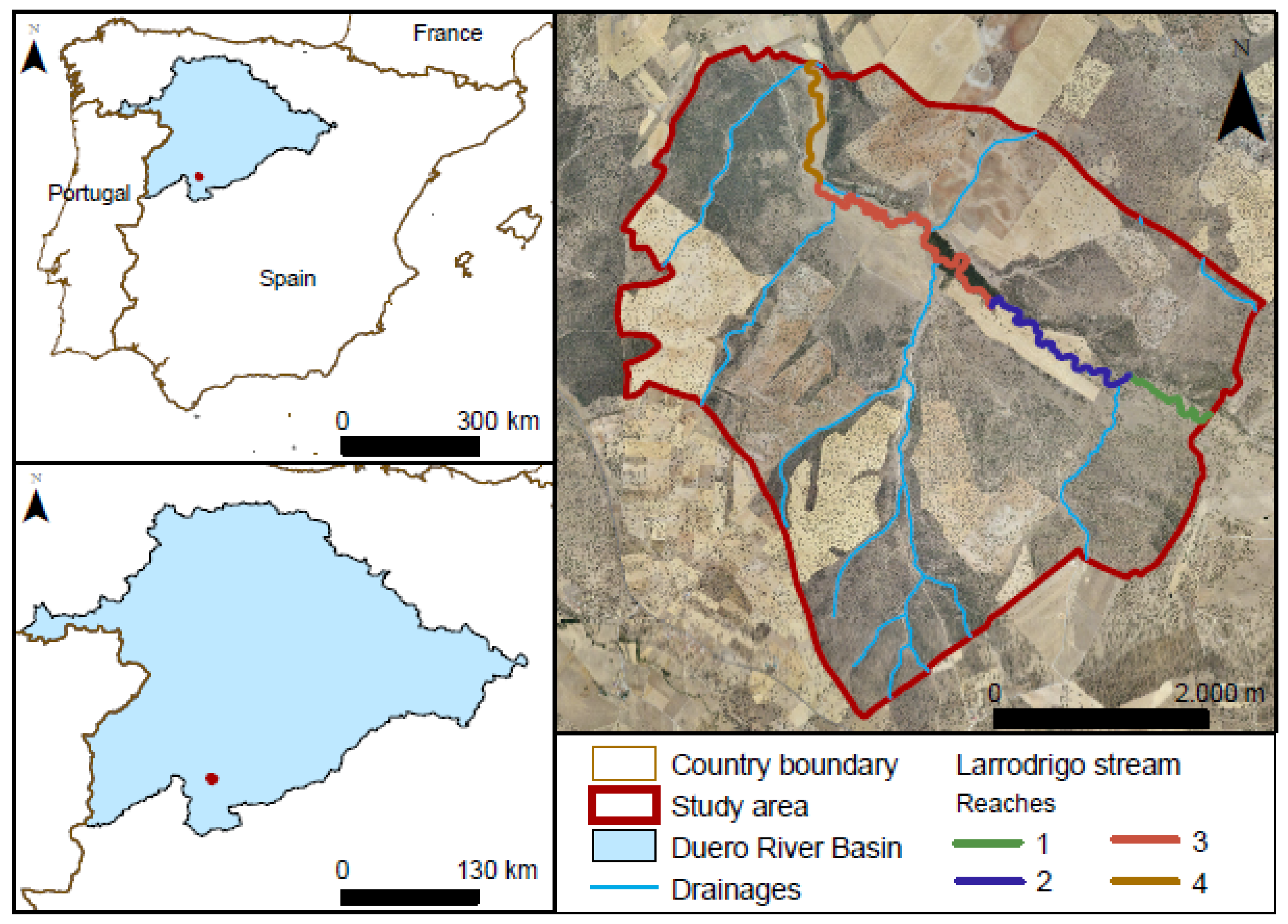
Considering the above, the aim of the present work is to develop a methodological framework to carry out an evolutionary study of the fluvial landscape in an intermittent water body on which agricultural activities have intervened. It is based on a detailed hydro-geomorphological–historical analysis, where erosional and sedimentary geomorphic elements are delineated to quantify morphological changes at a decadal scale in a floodplain. The method integrates several remote sensing techniques, including LiDAR datasets and analyses of available historical aerial and satellite imagery. The study was also supported by fieldwork that allowed for the collection of ephemeral and topographic evidence of water flow over the ground. Thus, the result is a practical method that can be applied in different holistic environmental studies where the fluvial landscape is an element of valuation. The formulated methodology was applied in the Larrodrigo stream, located in the Duero River basin, Salamanca, Spain (
Figure 1). This stream is categorized as a Natural River waterbody and is part of the Tormes River sub-zone. It is an intermittent waterbody, with a maximum flow of 0.6 m
3/s and a minimum of 0.05 m
3/s under normal conditions, with surface runoff and infiltration rates of 2.26 mm/year and 27.13 mm/year, respectively [
20].
This sector is covered by the geological cartography elaborated by the Geological and Mining Institute of Spain (IGME) at a scale of 1:50,000; however, there are no geomorphological maps of the study area. In this case, the most accurate geomorphological information is available in the surface formation sheets contained in the geological report at a scale of 1:100,000.
2. Methods
The methodology was developed under three main phases consisting of detailed hydro-geomorphological mapping of the study area, physical characterization of the basin at regional and local scales, and evolutionary analysis of the fluvial environment, which are further detailed below.
The hydro-geomorphological mapping consisted of the cartographic delimitation of the geomorphic elements generated by the water flow over the terrain at a scale of 1:1000. For this purpose, a terrain analysis was carried out using high-resolution LIDAR data, which were obtained from the Spatial Data Infrastructure of the Junta de Castilla y León (IDECyL), with a resolution of 1 m. From this, the DTM, profile, curvature, terrain orientation, shading models, and reclassified slopes were generated by using the Spatial Analyst tools available in ArcGIS 10.8 (
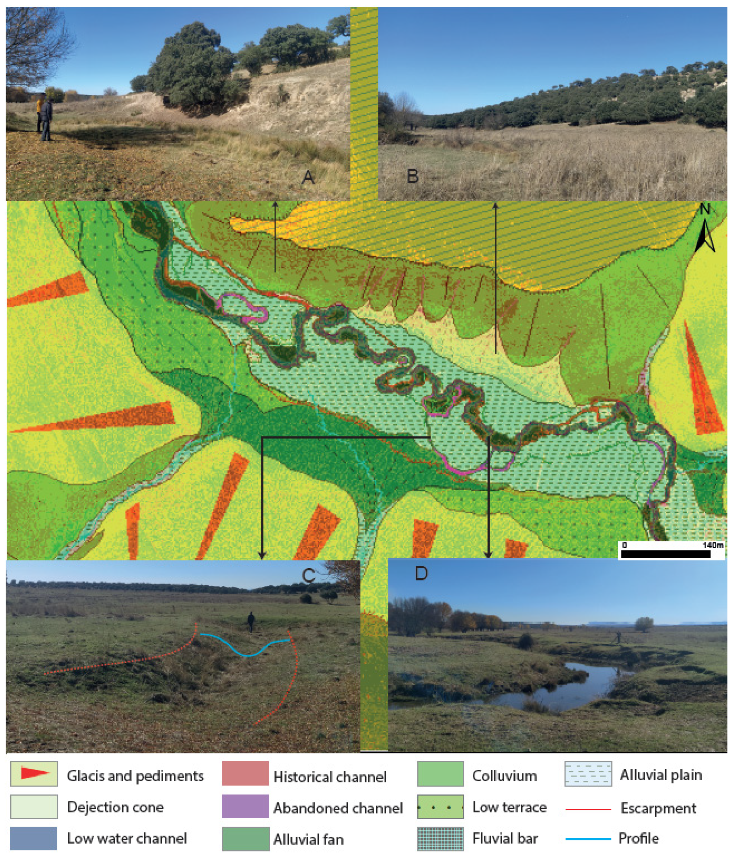
Figure 2). Through the generated models, changes in terrain such as flat areas, slopes, structural surfaces, and alluvial units were identified. The discretized DTM and slope models were used to identify different features such as height changes between structural surfaces and terraces, typical alluvial fan curvatures, limits to floodplain extents, and major or degraded escarpments. Orientation models are especially useful for identifying transverse floodplains, as well as flow directions. In this way, the shaded raster allows us to visually reconfirm the boundaries of surface formations, especially glacis, terraces, and structural surfaces.
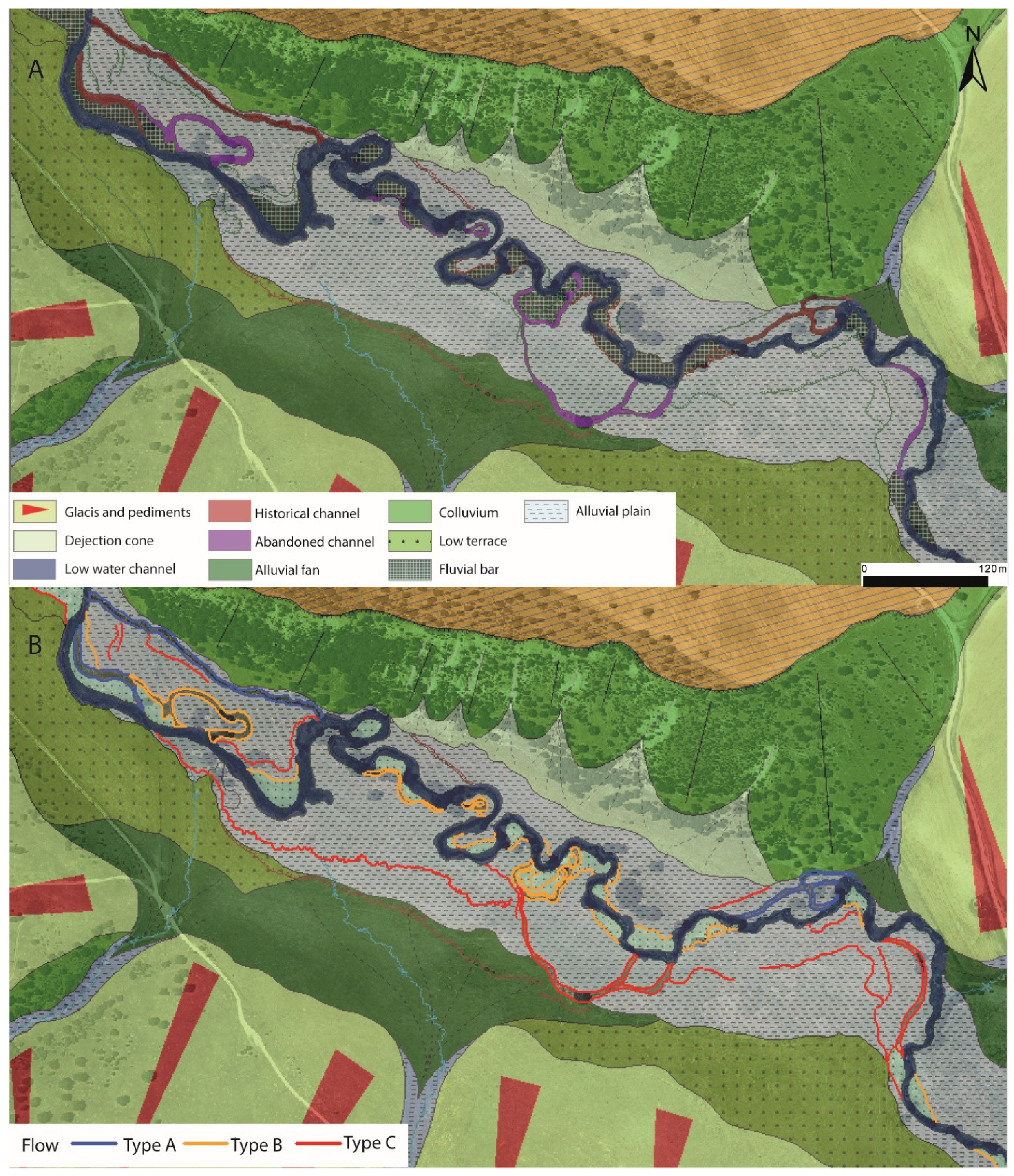
Based on these models, geomorphic elements were classified into different groups, differentiating the units associated with sedimentary and erosion processes. Erosion geomorphic units were delimited under four categories: low-water channels, secondary drainages, abandoned channels and historical channels. Depositional forms were set apart into low terraces, colluviums, structural surfaces, alluvial cones, fans, bars and plains. More details on the methodology can be found in Lombana and Martinez [
12] (
Figure 3).
Subsequently, secondary, abandoned, and historical channels were categorized into Type A, B and C flows [
21]: (a) Type A flows are those channels that in recent years have presented flows associated with low return periods (less than 5 years); (b) Type B drainages are related to higher return periods, and although surface flow is not directly observed, riparian vegetation can be found adjacent to its course; (c) Type C flows correspond to channels that could eventually present a flow of water in high return periods (greater than 50 years) and are associated with fluvial escarpments. This classification was made considering current water flows, which can be identified using high-resolution aerial imagery. In this case, the most up-to-date images were used; these were obtained from the National Aerial Orthophotography Plan (PNOA), provided by the National Geographic Institute (IGN) of Spain. In the photogram, it was possible to observe the sheets of water (out of low-water channels), as well as the riparian vegetation and/or escarpments generated by old streams.
The previously identified landforms were later verified in the field according to the ephemeral and topographic evidence present, including floating deposits, exposed fluvial sediments of poorly developed or absent soils and escarpments (
Figure 4).
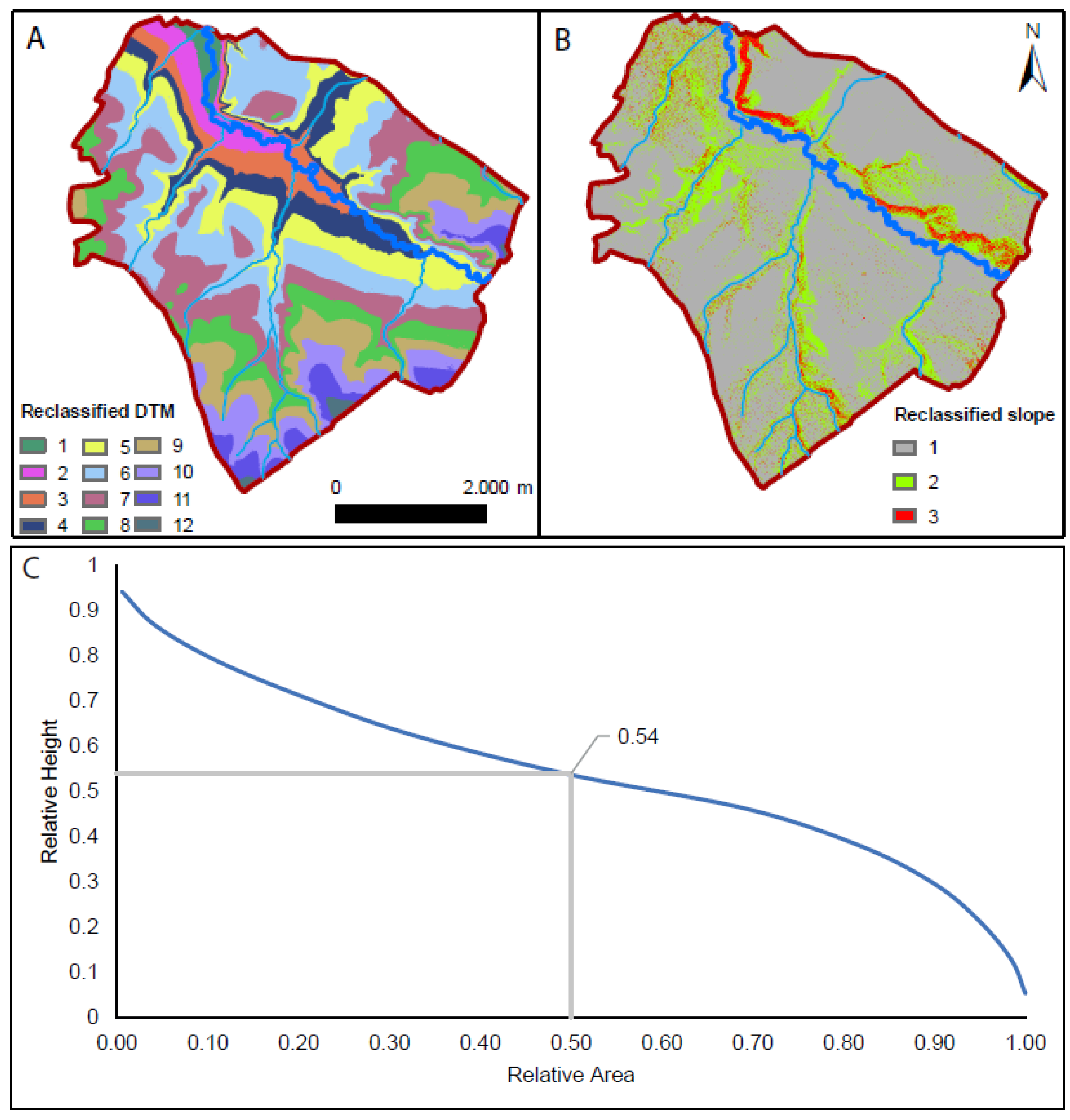
Subsequently, a morphometric analysis was carried out in order to describe some terrain physical characteristics at both regional and local scales, which are directly related to the fluvial dynamics of the system. Accordingly, the relief was initially characterized by calculating the area, minimum and maximum height, slope and altitude distribution (
Figure 5). The DTM previously generated and the Surface Analyses Tools in ArcGIS were implemented for this purpose. Altitude distribution analysis was carried out by using the hypsometric curve. In this case, the hypsometric integral (HI) was calculated using Equation (1) [
22,
23], and the cumulative height versus the cumulative area was plotted considering 12 classes (
Figure 5A). The mean slope of the study area was determined by reclassifying the previously obtained slope raster into 10 classes (
Figure 5B).
Emean = Mean elevation (m)
Emin = Minimum elevation (m)
Emax = Maximum elevation (m)
In addition, relief characterization indices, such as the Relief Ratio (Rhl) [
24], Relative Relief Ratio (Rhp) [
22], and Melton Ruggedness Number (MRn) [
22], were calculated using Equations (2)–(4), respectively.
The drainage network was characterized by calculating the stream order by Strahler (N), the sinuosity index of the longest flow path (S) (Equation (5)), and the average slope of the main channel (P) (Equation (6)) [
25]. For this, the main channel layout was traced over the slope and orientation models previously generated, following the line of greatest slope and depth, considering the sheet of water visible in the most up-to-date image (the 2017 orthophoto).
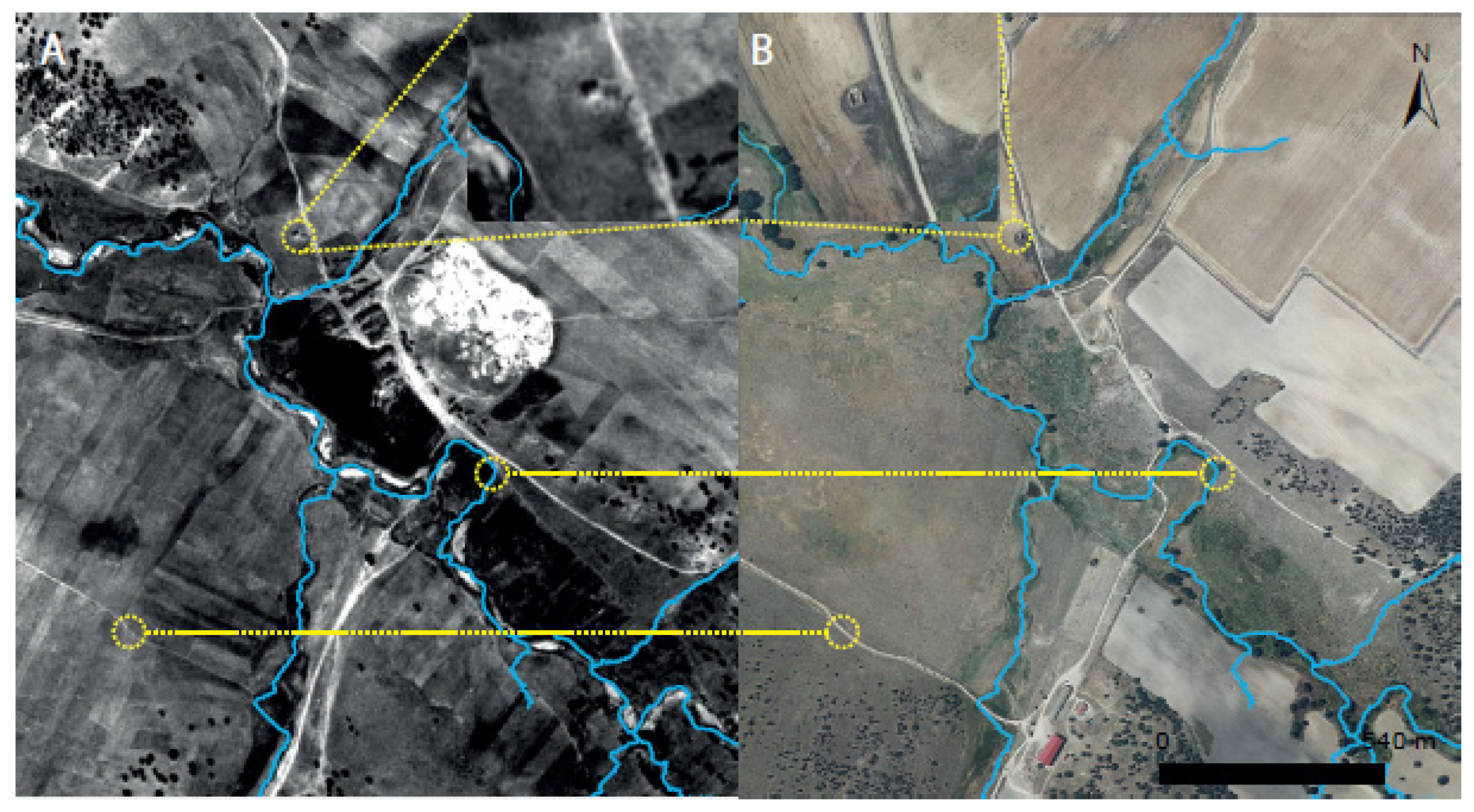
An evolutionary study of the fluvial landscape consists of recognizing the generalized movement of the main channel during the most recent decades by analyzing historical images [
16]. To this end, photograms of the study area were used—in this case, from the years 1902, 1957 and 2017, which are available in the IGN archive. These images were preprocessed in ArcGIS for later use. In the case of the 1902 frame at a scale of 1:25,000, the geographic projection was transformed to that used in the study (ETRS1989 Zone 30). The 1957 image was obtained from the so-called American Flight with an approximate scale of 1:32,000. This was georeferenced according to control points established near the area of interest, in order to reduce georeferencing errors [
26]. Areas that have not been modified in the topography, such as buildings, road crossings, and water reservoirs, were selected, having as a reference the 2017 orthophoto (
Figure 6) [
16].
The main channel of the stream was plotted on the previously processed historical images with a polygonal shape. For practical purposes, the study sector was divided into sections to analyze in detail the variations in length, width, and sinuosity indices over time in the main channel (Equation (5)). In this case, four sections were defined (
Figure 1). Then, the differences in the width of the main channel in 1957 and 2017 were quantified by applying a Symmetrical Difference analysis, available in the Overlay toolset of ArcGIS 10.8.
Abandoned and historical channel escarpments and fluvial bars were also identified cartographically, following the sequence of sedimentation–erosion zones between 1957 and 2017 [
15,
27]. The topographic evidence was verified on the slope model, curvature, and topographic evidence collected in the field, as previously performed (
Figure 4).
Thus, the identified surfaces were classified according to sedimentary or erosional processes where three categories were established: (a) accretion zones, (b) zones with historical erosion, and (c) zones with current erosion. Accretion zones refer to areas where the main channel was once located and which now belong to depositional zones. This category also includes river bars and abandoned channels. The areas classified as current erosion zones correspond to new surfaces covered in 2017 by the main channel as compared to 1957. On the other hand, historic channels were classified as historical erosion zones, as were areas of overlap between the historic main channel and the present channel.
3. Results
In accordance with the above, surface formations associated with the modeling of low slopes were delimited in the study area and were called Regularized Hillsides. These are characterized by the movement of material by diffuse surface streams that are only capable of transporting fine sediments that increase the hillside deposits, maintaining slope values between 3% and 5%.
Structural surfaces were delimited in the eastern zone, characterized by slopes of less than 3% and heights of more than 921 meters above sea level. These correspond to the high terraces of the Tormes River.
There are also accumulations of solids generated by ephemeral streams that deposit their solid load when the slope changes, forming alluvial fans and cones. On the recategorized DTM, it was possible to identify fan foot radii between 50 m and 650 m. These were identified mainly on the right bank of the Larrodrigo stream (
Figure 7).
In addition, asymmetric alluvial terraces were identified connected to the alluvial plain. These have marked intermediate scarps and flat surfaces with slopes of less than 3% and heights between 2 and 3 m, with one level on the right bank and two levels on the left side.
Through channel analyses, it was recognized that abandoned channels are mainly located at the left bank of the current low-water channel, which were reclassified as Type C flows, as can be seen in
Figure 8.
The morphometric parameters estimated in the study sector and the main channel according to current cartographic information are summarized in
Table 1.
According to the low Rhl value, which represents a measure of the average decrease in elevation per unit of axial length, and the main slope of 0.06, it can be concluded that the study area has a low relief. This is also supported in the low values of Rr, which represents the variation in altitude in a unit area with respect to its local base level, and the low Rhp of 0.004 [
17]. Besides this, the low value calculated for MRn suggests that the basins are less prone to erosion phenomena and have a structural configuration intrinsically associated with relief and drainage density [
28].
The hypsometric curve (
Figure 5C) varies due to the tectonic and geological characteristics of each analysis surface, so it can indicate that the study area presents an important part of its surface in areas of relatively medium relief. Accordingly, the curve obtained is representative of medium developed drainage areas that are in a mature state or with equilibrium conditions [
25], which can also be seen in the HI value obtained [
17].
The current low-water channel is approximately 8 km long and is characterized by a sinuous character, especially in
Section 3, where it has a higher sinuosity index and the widest lateral divagation area (
Table 2).
Thus, in contrast to the analyzed geomorphic units, the equilibrium stage in Larrodrigo can be represented by the presence of denudation processes in the Regularized Hillsides, the abandoned meanders formed in the alluvial plain, and the sinuosity index of the low-water channel.
In comparison with the fluvial configuration of the water body in 1957, differences were identified in the path and length of the main channel, presenting a smaller extension than the current one with a difference of 189 m and a lower sinuosity index (
Table 2).
Regarding the classification made according to sedimentary or erosional processes present in the stream,
Figure 9 shows the results obtained. Considering the area occupied by the low-water channel in 1957 and 2017 (
Table 3), a total of 44,589.6 m
2 was maintained, abandoning 22,349.2 m
2 of the area identified in the American flight. Thus, it can be specified that the low-water channel increased its coverage by 22,746.6 m
2 in 2017.
The different processes of lateral riverbed divagation lead to the abandonment of meanders by either gradual (chute cut-off) or abrupt (neck cut-off) mechanisms [
29]. As can be seen in
Figure 10, in
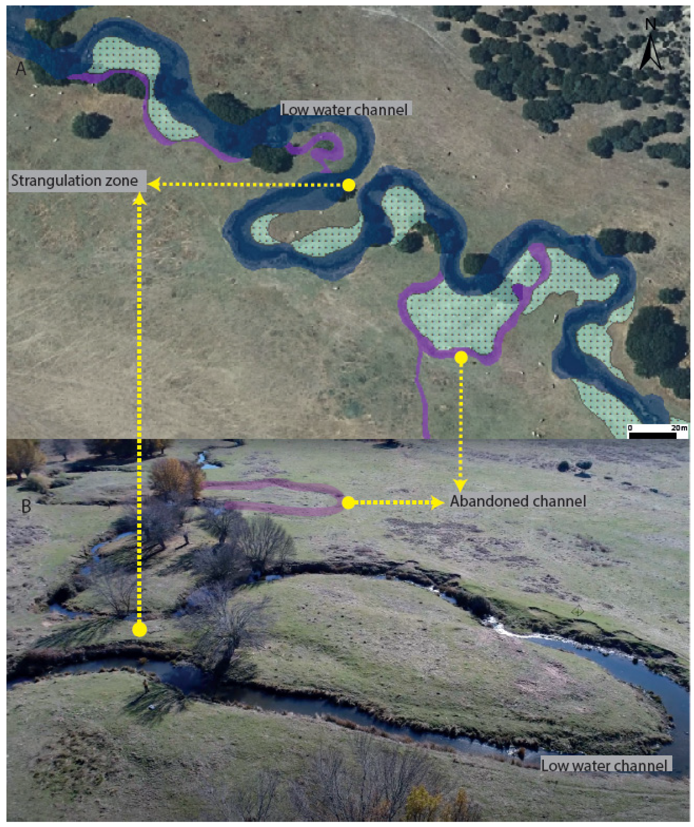
Section 3, the lateral displacement towards the right bank of the river is prominent. It has left abandoned meanders in its path, evidencing the occurrence of abrupt strangulations in the stream. These abandoned meanders are between 1.5 and 2 m deep according to evidence collected in the field (
Figure 2). Due to the curvature present in some sectors and the search for the base level of the stream, the future strangulation of other meanders is expected (strangulation zone in
Figure 10).
Thus, in general, the Larrodrigo stream flows towards its right bank, probably following the general displacement of neo-tectonic origin produced by the adjustment of the Central System (Sierra de Béjar) where the stream is located, as described by other authors [
3].
However, the presence of fluvial fans modifies the trend of this movement, causing the channel to move towards the left bank in some sectors. This dynamic is evident in
Section 2 of the channel, where an alluvial fan approximately 580 m wide has caused the lateral displacement of the channel towards the left bank, leaving abandoned channels in its path (
Figure 7).
Taking into account the intermittent hydrological regime of the water body, it can be said that the fluvial dynamics of the Larrodrigo are probably conditioned more by the geological processes of the area than by the sedimentation and erosion processes generated by the flow of the main channel, which, on average, does not exceed 0.05 m3/s. At the same time, agricultural activities do not seem to have a great impact on the evolution of the fluvial landscape, considering that the displacement of the main channel towards the right bank is probably mainly conditioned by the tectonic displacement of the area.
4. Discussion
The methodological framework formulated in this study allowed the detailed geomorphological characterization of the current state of the alluvial plain of an intermittent water body after intervention by anthropogenic activities. For this purpose, high-density LiDAR points and different remote sensing techniques, such as aerial photogrammetry, were used. This analysis also included morphometric variables that account for the fluvial dynamics of the system, such as the distribution of heights and slopes, relief ratios, and the sinuosity of the main stream [
30,
31,
32].
It was possible to determine and characterize the generalized movement of the main channel at a multitemporal level, using planimetries from the beginning of the 20th century and high-density aerial orthophotos from 2017. This followed the sequence of sedimentation–erosion zones in the stream. Thus, the method allowed us to study the horizontal movement of the geomorphic elements, differentiating in detail those zones denominated as current erosion areas, accretion zones and historical erosion zones. It also permitted us to identify different mechanisms of meander abandonment generated by the lateral displacement of the water body, which, in turn, provided information regarding future strangulations.
Thus, by relating morphometric parameters and geomorphic units present in the terrain, as well as the movement of these units, it was possible to determine the main drivers in the evolution of the fluvial landscape in an intermittent waterbody.
For further research, it is necessary to establish erosion—sedimentation volumes for the formulation of possible models of landscape evolution [
4]. Similarly, considering the extensive intervention in river systems, as is the case of the water body studied, future studies should consider the analysis of other environmental variables; these could include biotic parameters such as the dynamics of the movement of livestock, considering their direct influence on the physico-chemical composition of the soil and vegetation [
1].
The results of this methodological approach provide input for decision making regarding land use planning and the management of water bodies, making it possible to delimit intervention actions in accordance with the zoning of the fluvial space.
5. Conclusions
The methodology implemented in this study allowed for evolutionary analysis of the fluvial landscape of a highly modified water body through the study of the different geo-forms of the terrain, using high-level surface data.
Planimetries and various photogrammetric resources were used to identify the generalized movement of a river course. In this aspect, the process included a high level of field work to verify the findings made in the office.
For further studies, it is important to evaluate the inference of biotic variables in the dynamics of the fluvial current, considering the high level of agricultural and livestock intervention.
Therefore, for future intervention actions in the studied area, the results constitute a reference input for the establishment of environmental management measures, both for the conservation of water resources and for the appropriate management of soil.


