Article

Integrating Landscape Pattern into Characterising and Optimising Ecosystem Services for Regional Sustainable Development

1
Department of Public Management-Land Management, Huazhong Agricultural University, Wuhan 430070, China
2
College of Urban Economics and Public Administration, Capital University of Economics and Business, Beijing 100070, China
*
Author to whom correspondence should be addressed.
Submission received: 1 December 2021 / Revised: 4 January 2022 / Accepted: 7 January 2022 / Published: 17 January 2022
(This article belongs to the Topic Climate Change and Environmental Sustainability)

Abstract

:
Humans benefit from ecosystem services (ES) and profoundly influence the ecosystem in rapid urbanisation and large-scale urban sprawl contexts, especially at the landscape level. However, the impacts of landscape pattern, the driving mechanism of sub-ES and the spatially explicit regional optimisation, have been largely ignored. In response, to the present paper explores two primary aspects: the relationship among ES, landscape pattern, urban income and agricultural output, and the regional governance of optimised ES values (ESV), using the Wuhan urban agglomeration as a case study area. The survey method is employed in obtaining the adjusted magnitude matrix of land use and ecosystem services. Spatial regression analyses are conducted on each ES, including food provision, climate regulation and soil maintenance, with socio-economic indicators and landscape pattern index as explanatory variables. Finally, geographically weighted regression and scenario analyses are conducted on each sub-ESV to generate adjusted coefficients in each county for ESV regulation. The results show that urban per capita disposable income and agricultural output significantly contribute to ESV change, with the former being negative and the latter being positive. A highly aggregated landscape also produces reduced ESV, particularly in soil maintenance and gas and climate regulation. We summarise the ESV in 2020 and in the period after adjustment in different administrative counties. Provision, regulation and culture ecosystem benefits substantially increase when attempts are made to lower the landscape aggregation pattern by 1%. In general, counties and county-level cities have the largest ESV, with food provision as the optimum ecosystem benefit. Districts in the capital city show an immense growth in provision and regulation, and county-level cities show the highest growth rate in cultural service. Integrating the landscape pattern into characterising and optimising ES, provides references for regional governance on land-use planning and socio-economic development, which is vital to sustainable regional development.

1. Introduction

Humans benefit from ecosystem services (ESs) and profoundly influence the ecosystem in the context of rapid urbanisation and large-scale urban sprawl, especially at the landscape level [1,2]. All ESs are widely recognised as provision, regulation, maintenance and cultural and recreational services, which are important for the well-being and sustainable development of humans [3,4,5]. In return, the demand for social and economic advancement is actively transforming the regional landscape, thereby affecting ESs [6,7]. The comprehension of linkages among ESs, landscape pattern and socio-economic development help elucidate the driving mechanism underlying spatio-temporal ES changes, thus leading to additional pragmatic decisions on ecosystem management [8]. Rural areas in China are generally the most sensitive and vulnerable regions, in which agricultural sector development and farmer benefits tend to be offset for city development. In this process, the rural landscape has experienced dramatic changes that raise concerns on the relationships between ESs and landscape pattern in a rural socio-economic context.
Ecosystem service has been comprehended by scientists from a wide range of disciplines, and they have implemented multiple studies related to ES issues, such as the spatio-temporal patterns of comprehensive ES values (ESVs) and their underlying driving mechanisms, the relationship between landscape pattern and ESVs and the uncertainties in landscape ecology and ecosystem service. Ehrlich et al. (1981) first proposed the concept of ESs as an ecosystem function and environmental service [9]. Later, in ecology and sustainable development, ES is defined as the benefit received by humans from their interactions with ecological structures and functions [10,11]. In sociology, Jericó-Daminello et al. (2021) regarded ESs as ecosystem contributions combined with anthropogenic contributions, and they have impacts on ecosystems and benefit the social system [12]. Based on the understanding of the concept of ESs from multidisciplinary studies, it can be considered that ESs are the attributes, processes and functions of nature that directly or indirectly benefit human beings, through the functioning of ecosystem and natural assets [13,14]. In general, land use and land cover change are closely related to subsequent ESV change. Urbanisation, urban expansion, socio-economic development and human activities are supposed to be important drivers of ES changes. In China, total ESVs continuously declined in 1998–2008, and ESVs for regulation, culture, support and provision experienced a further decrease during 1988–2000 and 2000–2008, respectively [15]. Fang et al. (2021) depicted land use and ESV dynamics in the rapidly growing metropolitan area of the Yangtze and Yellow River Basins, and discovered that human activity intensity and population density are likely responsible for the overall decline in regional ESVs [16]. Abera et al. (2021) assessed ESV changes by connecting observed land use dynamics with ESV evaluation, and found forest land has been decreasing from 1986 to 2017, whereas the cropland has shown an increasing trend and this is driving a negative overall trend in the provision of ESs in southwestern Ethiopia [17]. Ketema et al. (2021) developed an ecosystem service supply rate and supply–demand ratio to construct the values of nature in supplying different ESs and indicating their use for human survival in the south-eastern escarpment of the Ethiopian Rift Valley [18]. The results revealed that a deficit in the status the provisioning of ecosystem service supply in the study region is not balanced with the existing ecosystem service demand. The demographic variables in rural areas, such as human population, population density, and number of villages, also threaten multi-functional landscapes and reduce the capacity to deliver ESs [19]. The effect of landscape pattern on ESs has emerged as an appealing research topic because of the exploration on spatial organisation in the landscape, along with associated landscape modifications from rapid and slow land cover changes [20]. The decreased variation in a landscape leads to different resistance to ecosystem service flows, such as landscape connectivity and permeability, but the provision of services then requires flows of species, humans, or matter to connect supply and demand areas [1]. A previous empirical study (i.e., Jiang et al. (2022) [21]), showed that ES provision is positively and negatively related to the amount of vegetation and the degree of fragmentation in an area, and that a multi-functional landscape reinforces local food production and enhances biodiversity and essential ESs [22]. Local landscape structures have been discovered to affect supply and compatibility across multiple ESs [23], and the high value area of flood mitigation have been found to be highly correlated with the spatial configuration of water body and woodland [24]. Moreover, landscape heterogeneity likely benefits a small but significant number of key farmland species and ESs [25]. With respect to uncertainties in ES studies or landscape analyses, the complexity of the landscape and the natural system [26], case study peculiarities [27] and data and methodological uncertainties all inherently affect ESV characterisation and modelling. The locally justified ES scoring method and the incorporation of stakeholder knowledge and perspectives have been applied to communicate uncertainty and improve accuracy [28,29].
Regardless of the comprehensive studies on ESV characterisation and analysis, the refined analysis on each ES and on spatially explicit approaches have occasionally been applied in ESV modelling and governance. In general, ES or benefits can be categorised into food and freshwater provision, soil conservation, hydrological adjustment, gas and climate regulation, natural heritage and landscape aesthetic value and culture and entertainment. These benefits are important for the survival of mankind and for well-rounded sustainability. These benefits also have trade-offs and distinctions that differentiate the extent to which socio-economic factors influence each benefit and that potentially provide references for follow-up regulation and governance. However, most scenario analyses on ESVs concerned with land use, landscape pattern effects and socio-economic development have hardly been utilised in optimising regional ESVs. Differences in the driving mechanism underlying various benefits and the spatial heterogeneity of the contribution of landscape pattern and socio-economic development help manage a series of uncertainties and provide information on regional ES governance. Thus, we adopt spatial modelling to analyse the driving factors for the change and regulation of each ESV in the Wuhan urban agglomeration, coupled with a survey and landscape pattern analysis. Section 2 of this research introduces the study area and methods, Section 3 provides the results and Section 4 includes the discussion and conclusion.

2. Materials and Methods

2.1. Study Area

The Wuhan urban agglomeration is located at the eastern part of Hubei province and along the middle reaches of the Yangtze River in central China. Administratively, there is one sub-provincial capital city, Wuhan, and 8 prefectural cities in the Wuhan agglomeration, and it is thus also been renowned as “1+8” urban agglomeration. With a permanent resident population of 32 million and an area of 57,908 km2 in 2020, Wuhan agglomeration has experienced rapid socio-economic development as its GDP surpassed 2636 billion that same year. The reasons why we chose Wuhan agglomeration as the case study area are as follows.
First of all, Wuhan agglomeration is one of the pioneering urban agglomerations with the policy of resource conservation and environment-friendly construction in China. Apart from the Yangtze River, a number of lakes and rivers occupy large areas that are vital for ecological conservation. In the past several decades, it has also experienced tremendous land-use and landscape pattern changes because of rapid industrialisation and urbanisation. In 2020, the expansion area of construction land reached 1523.49 km2, which is 2.5 times that in 2000, in the Wuhan agglomeration. Secondly, the Jianghan Plain has been regarded as the grain production base, and it sits in the western area of the Wuhan agglomeration. With its physical advantages, agricultural development is essential in the Wuhan agglomeration. In 2020, arable land and forests and grasslands occupied 49.10% and 40.52% of the total area, respectively (Figure 1). Secondly, the Millennium Ecosystem Assessment (MEA) report stated that the ecological services and values were not recognised enough in landscape planning and management [30]. It is worth noting that the crops planted in the Wuhan agglomeration are mainly rice, wheat, cotton and rape. In 2020, the total planting area of crops reached 30,620 km2 in the Wuhan agglomeration. Among them, rice, rape, wheat and cotton are the four crops with the largest planting area, accounting for 35.92%, 14.19%, 8.03% and 2.90%, respectively. In the last 10 years, the sown area has been reduced by 10.26%, especially the cotton planting area has reduced by more than half, while rape has also fallen by one-third. The rural landscape pattern has undergone drastic changes. Hence, taking the Wuhan agglomeration as a research area is helpful to explore the relative value of ESs in the context of rural landscape. As a result, exploration of the spatial-temporal ecosystem service and its driving forces in the Wuhan agglomeration is of great importance for the sustainable land use and urban-rural development.

2.2. Methodology

2.2.1. Questionnaire for Retrieving the ES Matrix

Although the estimation of certain benefits [31] can be conducted through various approaches, establishing the relationship between land use and ES is critical in deriving ESVs. Site-specific characteristics should also be included. In general, ESs can be classified into the following categories: provision services, such as food and freshwater supply; regulating services, such as gas, climate and hydrological management; and soil maintenance and cultural services, such as culture and entertainment, aesthetic value and natural heritage. All ESs can be extended or retrenched, depending on local peculiarity to provide specific benefits to society. In the study area, we included all nine services in the three ES groups because these benefits are prevalent in the Wuhan agglomeration. The local community influences ESVs and thus sets the basis for modifying ES and land-use relationships. Costanza et al. (1997) first produced the matrix of land use and ESVs [3], and then Xie et al. (2003) applied it to China with certain modifications [32]. Later on, there were wide applications with various modifications, such as biomass-based [33] modifications; agriculture output-based [34]; economic value-based [35]; gas adjustment for construction land [36]; grain production- and food market price-based [37]; the benefit transfer method [38] and adjustment based on the socioeconomic factors [39], using expert or public opinion of local conditions [40]. Twenty experts were consulted in this study for deriving this matrix: two from government bodies; three each from Wuhan University; two from Huazhong University of Science and Technology; two from Central China Normal University; two from Zhongnan University of Economics and Law; three from the Chinese Academy of Sciences (CAS) and six from Huazhong Agricultural University. Apart from CAS, all universities and government bodies of consulted experts are based in Wuhan, guaranteeing expert proficiency. The experts from CAS have also completed projects in Wuhan or in other cities in Hubei provinces, and are thus familiar with study area conditions. All 20 experts were interviewed and asked to rate the importance of each ecosystem service to every land use. The experts were informed of the ES concepts, and they all possessed adequate knowledge on the relationship between land use and ES. The rating scale was set from 0 to 4, with 0 indicating no relative potential 4 indicating a high relative potential and 2 and 3 implying a medium relationship.

2.2.2. Global Spatial Modelling of ESVs

During the spatio-temporal change, the driving factors of ES change have been found to be complicated, and spatial dependence was observed. To further explore the driving mechanism of different ES types, we adopted spatial modelling for each ES according to provision, regulation and culture services.
The explanatory factors can generally be classified into socio-economic variables and physical attributes. We selected 11 socio-economic variables as potential explanatory factors with respect to the demographic features (i.e., population density and urbanisation rate), sectoral structure (i.e., proportion of the secondary and tertiary industry to total GDP) and other key economic attributes (i.e., GDP per capita, total agricultural output, per capita disposable income for urban and rural residents, total fixed asset investment and foreign direct investment and per capita total retail sales of consumer goods). The correlation and simple regression analyses are assumed to have been implemented in 2010, 2015 and 2020, to include variables with the highest correlation with ES and without the multi-collinearity problem. Most physical attributes are temporally invariant or possess slight variations, increasing the difficulty at which they adapt to frequent and continuous socio-economic changes. However, the landscape pattern that depicts spatial clustering or land use diffusion is changing because of rapid urbanisation and urban expansion. The spatial aggregation or fragmentation of the landscape has also been revealed to be correlated with the local biomass and genetic and species diversity, fundamentally affecting the ecosystem and its societal benefits. Therefore, we calculated a series of landscape metrics to identify landscape pattern effects on ES: patch density (PD), contagion index (CONTAG), aggregation index (AI), perimeter–area fractal dimension and Shannon diversity index (SHDI). Previous studies rarely considered spatial dependence in their attempt to further examine underlying ES factors. Bundle types of ES and clustered distribution patterns have been discovered in the Xilin Gol, from 2001 to 2014 [41]. Yohannes et al. (2021) also suggested that a management plan should be developed to address the spatial relationship in ES, because there is a strong positive correlation between hydrological ESs and supporting services [2], highlighting a strong synergetic relationship between the spatial and temporal. In this study, we tested the spatial autocorrelation of each and all ESs, to justify the existence of spatial auto-correlation. Under the hypothesis of spatial dependence in ESs, we employed spatial regression models to reveal driving factors and make comparisons. Spatial regression models generally have two types: the spatial lag and spatial error models. The spatial lag model assumes that neighbouring dependent variable values directly affect the value of the dependent variable and incorporates the spatially lagged variable in its specification, Equation (1). The spatial error model treats spatial correlation primarily as a nuisance and assumes that model errors are correlated across distances among observations, Equation (2). We performed a simple linear regression using the ordinary least square (OLS) method and the Lagrange multiplier (LM) test to choose between spatial lag and spatial error regression as the optimal model performance for each ES.
yi = α W yi + β Xi + μ
yi = β Xi + μ  μ = ρ W μ + ε
where yi is the ES value for each and all ES types; Xi denotes potential driving factors, including socio-economic variables and metrics from landscape ecology; α is the spatial lag coefficient; β represents the correlation coefficients for independent variables and μ is the error term and W is the spatial weight matrix. The first order rook contiguity weight was selected for this analysis.

2.2.3. Local Spatial Adjustment of ESVs

Preliminary ESV modelling and assessment aim to improve ESs and comprehensive sustainability in certain areas. Most regulation and scenario analyses regarding ES optimisation are concerned with land use change, leaving much potential for exploring and utilising landscape pattern effects. Previous studies confirmed that urban expansion, cropland encroachment and ecological land loss greatly impact ESVs with respect to land use structure. According to empirical studies [3,33,42], ES calculation is precisely based on areas of each land use type. Therefore, ES optimisation is achieved by adjusting the land use structure. However, the influence of landscape spatial distribution on ESs has scarcely been utilised in enhancing specific and integrated ESs. We are entering an era in which land use planning is oriented to “inventory planning” rather than “increment planning”. Thus, the spatial form of land use is highly likely to adjust for compact and intensive growth. We aim to improve ESs by changing the landscape pattern and conducting a scenario analysis.
The driving mechanism of ESs at each location potentially differs from one another. ES improvement also requires the consideration of spatial heterogeneity. Previous empirical studies assumed that factor contributions are spatially homogenous and that the regulation on improving ESs is generally comprehensive, hindering their interpretation of the spatial difference between ES modelling and optimisation, and reducing ES regulation accuracy. Spatial dependence and interaction have also been widely acknowledged. Thus, geographically weighted regression (GWR) is suitable for scenario analysis through landscape pattern regulation. GWR is a regression technique that allows locally weighted regression coefficients to move away from their global values, and the relationships between independent and dependent variables to achieve variation by locality. Specifically, GWR constructs a separate OLS equation incorporating dependent and independent variables of locations falling within the bandwidth of each target location. Equations (3) and (4) shows the GWR specifications.
yi = β0 + β1 x1 + β2 x2 + β3 x3 + … βni xni + εi
βi = ( XT Wi X )−1 XT
In this study, we use the fixed Gaussian kernel and golden bandwidth selection method to derive the varying coefficients.

3. Results

3.1. Matrix of Land Use and Ecosystem Service

The local matrix of land use and ES is obtained and standardised from 0 to 1, on the basis of the interview with experts and the statistical analysis. The results in Table 1 show that each ecosystem service (i.e., provision, regulation and cultural service) is distinctly relevant to every land use. Aside from cultivated land, which yields the highest score for food provision, water, forests and grassland are the three other land use types with the highest scores. Freshwater supply is most closely related with water, followed by forests and grassland. Forests, water and grassland are the top three land use types that significantly influence gas, climate and hydrological regulation. Soil maintenance in the regulation category is most strongly linked to forests and grassland, followed by cultivated land. Although construction land yields the lowest scores in terms of provision and regulation services, it obtains the highest in culture and entertainment. Finally, forests and water have the closest relationship with aesthetic value and natural heritage and diversity.
The relevance matrix is then transformed into the ESV equivalent per area matrix (Table 2), on the basis of research by Xie et al. (2003) [32], which regards one ESV unit as 449.1 CNY/hm2. The ranking of relationships between land use and ESVs are the same as that in Table 1. With the matrix and information on areas of different land use, calculating each ecosystem service value for the following modelling method is feasible.

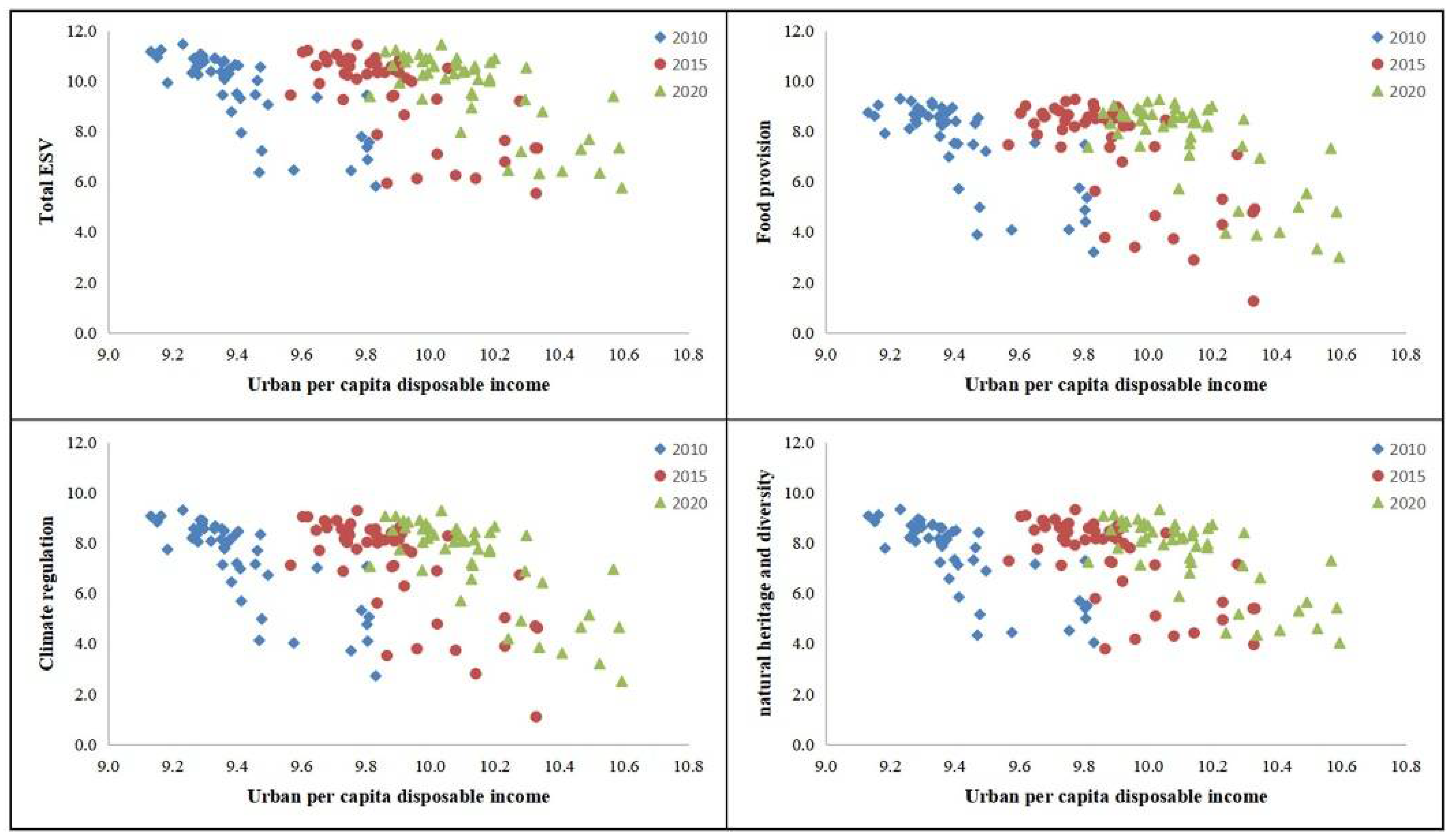
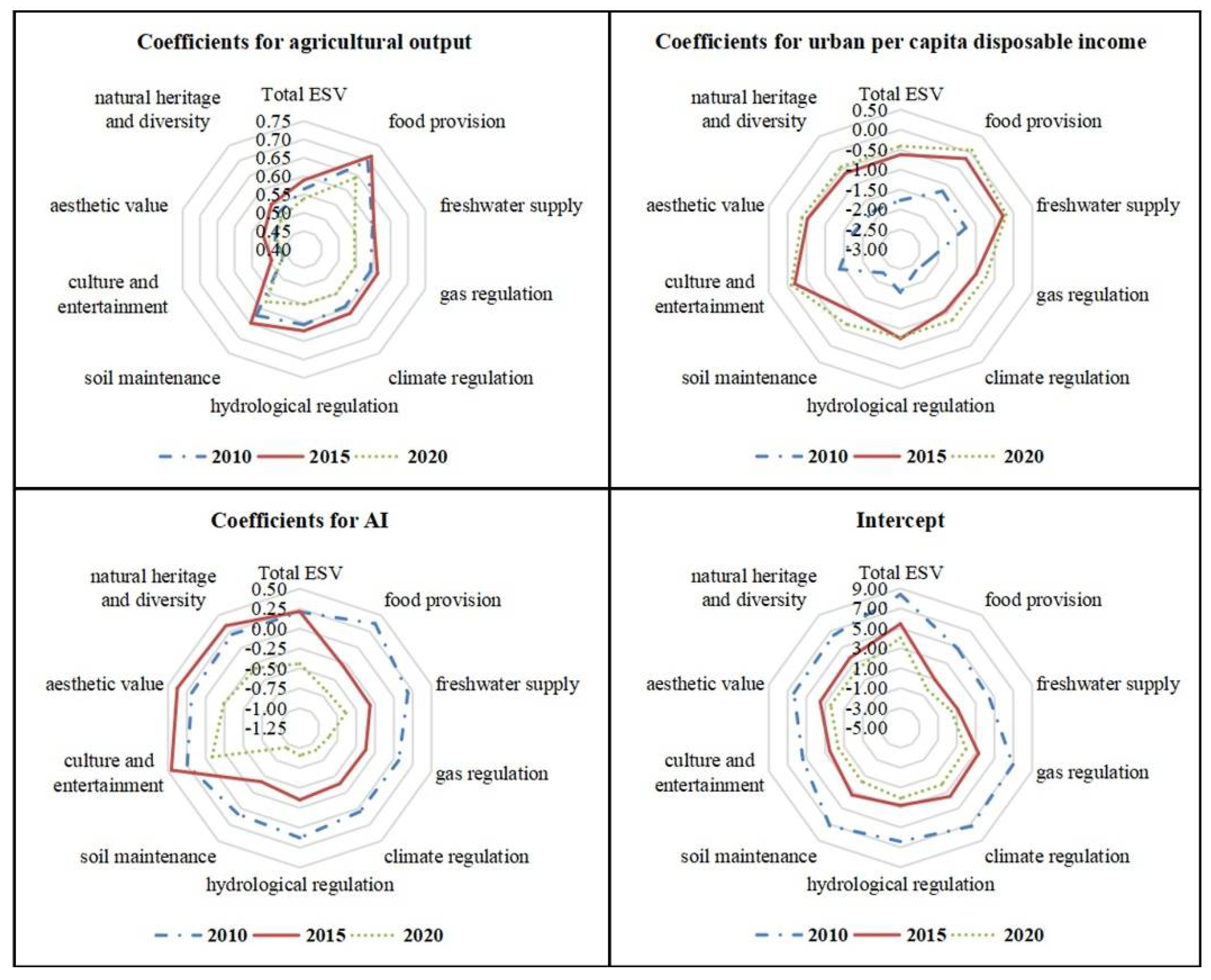
3.2. The Driving Factors for ESV Change

After the correlation and regression analyses, the factors of urban per capita disposable income, agricultural output and AI are selected as driving factors for further modelling. Scatterplots of urban per capita disposable income, agricultural output, AI and total ESV are created in logarithmic form. Figure 2, Figure 3 and Figure 4 illustrate the representative relationships for provision, regulation and culture and total ESV. In general, different ESs with the same driving factors exhibit similar patterns. The urban per capita disposable income and AI are negatively correlated with the ESV, whereas agricultural output positively influences it.
The scatterplots of urban per capita disposable income and ESVs (Figure 2) move towards increased x-axis values in 2010–2020, showing that urban per capita disposable income has increased, and that the ESV has slightly declined. The negative effects of urban per capita disposable income are highest on climate regulation, followed by food provision. Urban per capita income and total ESVs generate a modest negative slope. Specifically, in 2020, the 1% decrease in urban per capita disposable income generates a 6.61%, 6.23%, 5.36% and 5.71% increase in climate change, food provision, natural heritage and diversity benefits and total ESV, respectively.
The slopes in the scatterplots between agricultural output and ESV (Figure 3) declined in 2010–2020, implying a greater positive influence of agriculture output on the ESV in 2010–2015 than on that in 2015–2020. The correlation coefficient between the food supply and agricultural output is the highest, while the correlation coefficient between natural heritage and diversity and agricultural output is the lowest. A 1% increase in the agricultural output in 2010, 2015 and 2020, respectively, brings a 0.78%, 0.77% and 0.70% increase in food provision, a 0.75%, 0.74% and 0.69% increase in climate regulation and a 0.65%, 0.59% and 0.58% increase in natural heritage and diversity.
Similar to Figure 2, the scatterplots of AI and ESV (Figure 4) show a distinct negative relationship, with 2010 being the most negative. The climate regulation benefit is negatively affected the most, followed by food provision, total ESVs and natural heritage and diversity. A 1% increase in AI in 2010 has led to an 86.64%, 81.44% and 69.31% decline in climate regulation, food provision and natural heritage and diversity benefits, respectively. Although the correlation coefficient seems large, the AI range is constrained to 4.54–4.6. The effects of landscape pattern on ESVs also appear to be sensitive.
Differences exist among varying ESVs and explanatory variables. The urban per capita disposable income and AI exhibit negative correlation influences on different ESVs. The spatial coefficient is significant for all ESVs, with aesthetic value yielding the highest value and food provision yielding the lowest.
Figure 5 shows the correlation coefficients of the nine sub-ESVs and the total ESV for urban per capita disposable income, agricultural output, AI and spatial coefficients. The negative correlation coefficients of urban per capita disposable income for the three particular years attenuate for urban per capita disposable income, especially during 2010–2015. In 2010 and 2015, climate regulation has yielded the highest negative correlation coefficient, whereas food provision has yielded the lowest. In 2020, climate regulation has the most powerful negative influence, whereas food provision and hydrological regulation has the weakest. Rural per capita disposable income generally presents a significantly negative influence on regulation benefits and a weak influence on provision benefits.
The positive contribution of agricultural output on ESVs increased during 2010–2015, followed by an apparent decline in 2020. Within 2010–2020, the strongest positive influence of agricultural output on ESVs is under food provision, and the weakest is under culture and entertainment. Agricultural output greatly influences food provision but weakly influences culture and entertainment. The AI influences on different ESVs show an irregular pattern with the increase in all ESVs, during 2010–2015. The AI coefficients for culture and entertainment, aesthetic value, natural heritage and diversity and total ESV rise, whereas the rest declines. In the following five years, the AI demonstrates negative impacts on ESVs. The food provision yields the highest spatial coefficient in 2010 and culture and entertainment yields it in 2015 and 2020. The lowest spatial coefficient is yielded by climate regulation in 2010, soil maintenance in 2015 and 2020.
The spatial coefficients influences on different ESVs demonstrate a downward trend during 2010–2020, with climate regulation suffering the most powerful impact in 2010 and freshwater supply bearing the slightest. In 2020, the most powerful and the weakest influence transfer to aesthetic value and food provision, respectively, indicating that provision still suffers the most powerful negative influence.

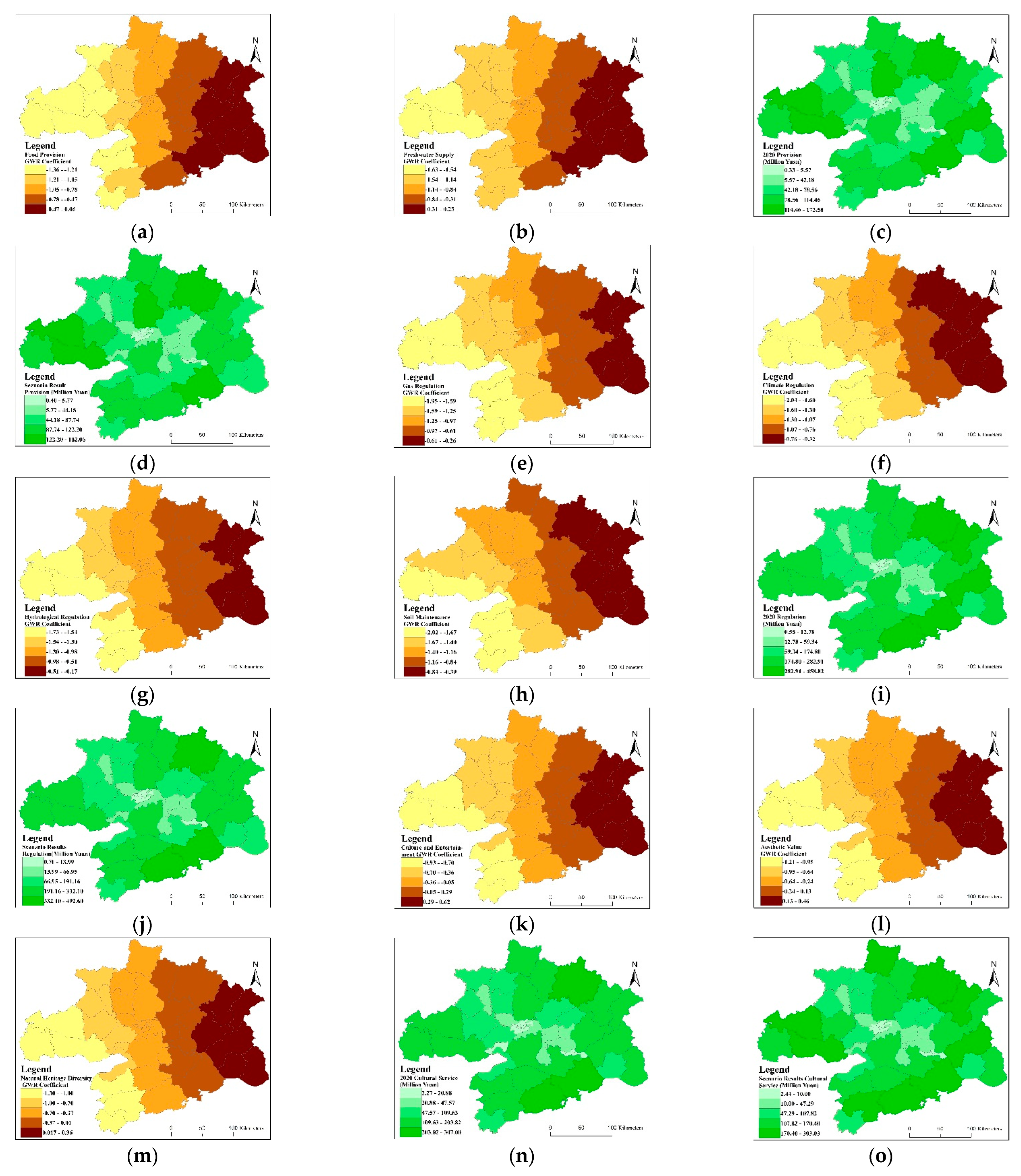
3.3. Spatial Adjustment of ESVs

The coefficients of AI and ESV, and the simulated ESV after a 1% decrease in aggregation degree, have exhibited spatial heterogeneity. Figure 6a–d illustrate the spatial distribution of food provision and freshwater supply coefficients generated from GWR, the spatial pattern of provision ES and the optimised provision of ESV when AI is reduced by 1%. Xiantao and Qianjiang are both county-level cities directly under the central government in the Wuhan agglomeration, and they yield the highest negative coefficients for food provision and freshwater supply, respectively. The coefficients range from 0.0619 to −1.3666 and from 0.2592 to −1.6333 for food provision and freshwater supply, respectively. In 2020 and in the simulated scenario, Macheng in north-east Wuhan yields the highest ESV, whereas Jianghan yields the lowest. Tianmen is a county-level city in the western area, and it exhibits the greatest ES growth when the AI is reduced by 1%.
Figure 6e–j illustrate the spatial distribution of gas regulation, climate regulation, hydrological regulation and soil maintenance coefficients generated from GWR, the spatial pattern of regulation services and the optimised regulation value when the AI is reduced by 1%. Tongcheng County in the southern Wuhan area has the strongest negative contributions for all regulation services, with coefficients ranging from −1.7382 to −2.0209. Yingshan County in eastern the Wuhan agglomeration has the weakest negative influences on all regulation services from −0.1789 to −0.3973 coefficients. In terms of the spatial distribution of regulation benefits in 2020 and after the adjustment, Jianghan District in western Wuhan still has the lowest value and the least growth, Macheng County has the highest value, whereas Chongyang County has the greatest growth.
Figure 6k–o illustrate the spatial distribution of the culture and entertainment, aesthetic value, natural heritage and diversity coefficients generated from GWR, the spatial pattern of culture ESs and the optimised culture value when the AI is reduced by 1%. The cultural services yield significant spatial coefficient ranges of −0.9369 to 0.6235, −1.2156 to 0.4638, −1.3053 to 0.3606 for culture and entertainment, aesthetic value, natural heritage and diversity, respectively. Yingshan County generates the slightest negative influence, similar to its result in provision and regulation services. Tongcheng County is located at the southern part of Xianning prefectural city, and it generates the most powerful negative influence. Similar to previous results, Macheng has the highest culture ESV in 2020 and after the adjustment. Different from the supply and supervision services, the adjusted cultural ESV of some counties has been reduced, and most of them belong to Huanggang prefectural City, which is located in the eastern part of the Wuhan agglomeration. By contrast, Qianjiang exhibits the greatest growth.
Table 3 summarises the ESV in 2020 and after the adjustment in different administrative counties. Provision, regulation and culture services substantially increase when attempts are made to reduce the landscape aggregation pattern by 1%. County-level cities and counties generally yield the largest ESVs in 2020 and after the adjustment, with food provision being the optimum ES. Districts in the prefecture-level city show a significant growth in provision and regulation services, and urban districts in Wuhan show the highest regulation growth rate. Although urban districts yield the lowest ESV, the growth rate is comparatively high after the landscape pattern adjustment. Under provision service, a higher gap exists between food provision and freshwater supply in county-level cities than that in urban districts, with food provision obtaining the increased amount. When the landscape is designed to increase in fragmentation by 1%, provision services increase at the highest growth rate of 12.55%, from CNY 39 to 44 million in capital city urban districts. Under regulation services, hydrological regulation yields the highest ESV, whereas climate regulation yields the lowest. County-level cities and counties distinctively have substantial regulation services in all four ESVs, and they experience the large increase after 1% aggregation level change. County-level cities yield the higher growth rate, whereas counties yield the lowest. In cultural services, not much difference is observed between the ESV of aesthetic value and natural heritage and diversity, which are higher than that of culture and entertainment, except in urban districts. Although cultural service ESV is high in counties, they present low growth rates after optimisation. Cultural service ESV increases at the highest growth rate from CNY 1402 to 1476 million in county-level cities, and from CNY 80 to 83 million in capital city urban districts.

4. Discussion

ES, as the benefits that humans receive from their surrounding environment, is inherently contributed to the sustainable development goals (17 SDGs) proposed by the UN decade in facing severe challenges of climate change, biodiversity loss and degraded ecosystems [43]. ESs can meet various human needs, in line with the numerous aspirations contained in the SDGs (e.g., Clean Water and Sanitation, Zero Hunger and Climate Action). The goal of clean water and sanitation can be realised through improving the ecological service of freshwater supply service; the goal of enough food is closely related to the ecosystem service of food provision and climate change is directed related to the ecosystem service of climate regulation [44]. It is declared by the United Nations General Assembly (www.decadeonrestoration.org accessed date 20 December 2021) that 2021–2030 was the decade that focused on the restoration of ecosystems [45]. Hence, it is imperative to refine the measurement on ESs, ponder the driving mechanism of ESs and explore the feasible approaches to improve ESs.
On the basis of the empirical studies and the local questionnaire, we derives the conversion parameter from land use area to different ESVs, and used the Wuhan urban agglomeration as the case study area to evaluate its ESVs. In general, the results produced in our study are similar to the those in other regions and cases worldwide, yet there are differences since land use distribution is different. For example, Hardaker et al. (2020) considered that the ecosystem service of forest land and cultivated land are basically the same in Wales, U.K. [46]. This is attributed to the fact that there is more fertile arable land in England, more general ecological protection measures and less damage to the ecosystem, which is different from the situation in our study area. The ecosystem service of forest land is higher than that of cultivated land in the Wuhan agglomeration. In this sense, it is discovered that there is also regional difference in terms of ES, due to the different physical environment and terrestrial ecosystem. In terms of the ESV calculation results, we used the average ESV of Ezhou City (one of the nine major cities in the Wuhan agglomeration) in 2015, as an example. Based on the conversion parameters, we calculated the result to be 3.60 million USD/km2, which is roughly the same as the 3.71 million USD/km2, by Xing et al. (2020) [47]. Therefore, the results in our study can be considered to be accurate and reasonable. Although the evidence and justifications already verify the effectiveness, the optimal approach is to implement a local field experiment to derive parameters integrated with observation data and previous studies.
This study aims to examine how landscape pattern influence is utilised as the medium for adjustment in optimising ESVs, to explore the idea that global and local spatial modelling are applied to generate regression results for analysis and optimisation. The primary contributions are based on two aspects that consider how landscape pattern affects ESVs, using spatially explicit modelling and analysis. Previous studies examined how landscape changes influence the terrestrial, aquatic and atmospheric environment and biomass because the fragmentation or aggregation of the landscape pattern determines the geo-bio-physical setting to some extent [48,49,50]. To explore the ways for adjustment in optimising ESVs through landscape patterns, we divided ES into three categories, namely, provision, regulation and culture. They all have close relationships with the biophysical environment, food production and also biodiversity conservation, forming the theoretical basis for the assumption that landscape pattern affects ESs [51,52,53]. We selected a number of metrics in landscape ecology to describe the pattern and process at patch and landscape levels. Some scholars also expanded the factors influencing ESs, including geographic factors [54] and socio-economic factors [55]. The landscape index is incorporated into the regression and scenario analyses because it is more pragmatic for landscape pattern adjustment than for socio-economic development. Finally, we determined three indicators, including urban per capita disposable income, agricultural output and AI. The regression model shows that urban per capita disposable income and agricultural output are highly correlated with ESVs, with negative and positive correlations, respectively. Achieving the ESV improvement implies a reduction in urban per capita disposable income and an increase in the agricultural output, which is impossible due to the promotion of urban livelihood and urbanisation processes. In addition, AI also shows a significant negative correlation with ESV, which conforms to the results from the study by Tran et al. (2022) in the Manawatu-Wanganui region of the North Island, New Zealand, and the study by Rolo et al. (2021) in 12 rural regions across 9 European countries, including Mediterranean, Atlantic, Boreal and Continental [56,57]. The relationship between ESV and landscape pattern have all been diagnosed. In this sense, adjusting the landscape pattern is a feasible approach as we enter an inventory planning era. In the context of spatial planning, the dispersed landscape patterns through mixed land use [58] and polycentric spatial form [59] to increase ESV is viable. As a result, the highlight of the influence on landscape patterns is pioneering and feasible.
The second contribution is related to the spatially explicit thought on ES modelling and optimisation. Previous studies generally attempt to optimise ESVs based on land use [60], which the spatial heterogeneity of the ecosystem change is seldom considered or applied. In recent years, the spatial correlation in ES seems to be an appealing issue gaining widespread attention and possessing uncertainties that require further explanation. Degefu et al. (2021) confirmed the spatial dependence and spatial autocorrelation of ESVs in Ethiopia [7]. Therefore, we attempt to consider spatial heterogeneity in scenario analysis. The optimised ESV has increased by an average of 8.3% through adjusting the landscape pattern. The typical spatial regression model assumes the existence of spatial influence either in dependent variables or in errors, which corresponds to spatial lag and spatial error models. The regression analysis is implemented in both forms, and the results are compared using the OLS method. The spatial regression model is proclaimed superior due to its improved performance and accuracy. Ultimately, the spatial error model is chosen for exploring the global driving mechanism on the basis of the LM test. The local spatial modelling technique, GWR, is implemented in this study, and the local spatial influences are important to generate varying coefficients for different observations. The spatial disparity of urban per capita disposable income, agricultural output and AI contributions on different ESVs in various places in the Wuhan agglomeration fully unfold in accordance with the regression results. Local regression should be implemented in the future as it compensates the shortcomings of global modelling techniques. When varying coefficients are produced, the local benefits of improved ESVs can be obtained through the AI adjustment. Inspiringly, the adjustment of the urban landscape through the spatial structure and function seems to be feasible in improving ESs [53,56]. Furthermore, it is true that in ecosystem benefits, it is not enough to take landscape pattern, rural development and living standards as the influencing factors. This requires a systematic strategy in which agriculture, industry and politics all need to be included in exploring the driving mechanisms. The improvement of ecosystem benefits requires the adjustment of specific factors and the consideration of spatial heterogeneity to discern feasible strategies. In addition, our method can be applied to evaluate local ESVs and analyse possible optimisation approaches through landscape patterns, such as China, Russia, and South America. These areas have a large amount of arable land, rivers and lakes, and diverse landscape types. The adjustment in optimising ESVs through landscape patterns can be applied in urban and rural planning, including the implementation of mixed land use and the shaping of multiple types of landscapes. The increase in ESVs is beneficial to improve ecological functions and realise the 17 SDGs, such as poverty alleviation, clean water and climate change.

5. Conclusions

The investigation on the spatio-temporal patterns of ESVs, underlying driving forces and pragmatic optimisation approaches are important to regional sustainability. Empirical studies have identified primary ESs and benefits, determined the primary socio-economic driving factors and proposed several regulation pathways. However, most studies are closely related to land use change and are comprehensively investigated. Employing the Wuhan agglomeration as the case study area, we attempted to analyse each primary ES in the context of food security initiatives, climate change concerns and green construction programs in China. The results find negative influences of urban per capita disposable income and AI, and the positive effects of agricultural outputs, with varying contributions to different ESs. Moreover, landscape pattern influence is explored and utilised as the medium for adjustment in optimising ESVs. Global and local spatial modelling are then applied to generate regression results for analysis and optimisation. The spatial adjustments on the ESVs are then performed through GWR and a 1% change in AI. The results also reveal that ES growth rates in the AI scenario analysis declined by 1%.
The limitations and recommendations of this study involve the in-depth interpretation of spatial correlation in modelling ESVs, and further policy implications of spatial adjustment for improving local ESVs. The spatial correlation in analysing the driving forces has been mentioned in previous studies, whereas the interpretation of how the neighbouring effect or the spatial influence in error emergences and changes remains unsettled. This gap is due to complicated courses during the spatio-temporal change that are difficult to systematically analyse. Uncertainties in the driving mechanism of the ESV changes and further experience should be accumulated to obtain improved explanation. Additionally, we applied spatial adjustments to ESVs through the change in landscape pattern, which is a method proven to have increased feasibility. Considering the constraints of urban and land use planning, the issue of how to transform the agglomeration pattern needs further exploration. The same issues are that developing countries need to take some measures to improve compensation after different ESs have been comprehensively improved, the change in the spatial heterogeneity of driving forces, and whether ESVs can be regulated and predicted in the future. In general, addressing these issues requires further collaboration with experts in fields, such as ecology, biology and sociology. The current study links the ecosystem change to landscape patterns with spatially explicit approaches.

Author Contributions

Conceptualisation, Y.L. and C.Z.; methodology, C.Z.; software, Y.L.; validation, Y.L., Z.L. and B.C.; investigation, Y.L., Z.L. and B.C.; resources, C.Z. and Y.Z.; data curation, Y.L.; writing-original draft preparation, C.Z.; writing-review and editing, Y.L., C.Z. and Z.L.; visualisation, Y.L.; supervision, C.Z. and Y.Z.; project administration, Y.L.; funding acquisition, C.Z. All authors have read and agreed to the published version of the manuscript.

Funding

This research was supported by the National Natural Science Foundation of China (41771563, 42171262), the National Social Science Fund of China (20ZDA086) and the Independent Science and Technology Innovation Fund Project of Huazhong Agricultural University (2662021JC002).

Institutional Review Board Statement

Not applicable.

Informed Consent Statement

Not applicable.

Data Availability Statement

Not applicable.

Acknowledgments

The authors would like to thank the anonymous reviewers for their valuable comments.

Conflicts of Interest

The authors declare no conflict of interest.

References

  1. Metzger, J.P.; Villarreal-Rosas, J.; Suárez-Castro, A.F.; López-Cubillos, S.; González-Chaves, A.; Runting, R.K.; Hohlenwerger, C.; Rhodes, J.R. Considering landscape-level processes in ecosystem service assessments. Sci. Total Environ. 2021, 796, 149028. [Google Scholar] [CrossRef]
  2. Yohannes, H.; Soromessa, T.; Argaw, M.; Warkineh, B. Spatio-temporal changes in ecosystem service bundles and hotspots in Beressa watershed of the Ethiopian highlands: Implications for landscape management. Environ. Chall. 2021, 5, 100324. [Google Scholar] [CrossRef]
  3. Costanza, R.; d’Arge, R.; De Groot, R.; Farber, S.; Grasso, M.; Hannon, B.; Limburg, K.; Naeem, S.; O’Neill, R.V.; Paruelo, J.; et al. The value of the world’s ecosystem services and natural capital. Nature 1997, 387, 253–260. [Google Scholar] [CrossRef]
  4. De Groot, R.S.; Wilson, M.A.; Boumans, R.M. A typology for the classification, description and valuation of ecosystem functions, goods and services. Ecol. Econ. 2002, 41, 393–408. [Google Scholar] [CrossRef] [Green Version]
  5. Costanza, R.; De Groot, R.; Sutton, P.; Van der Ploeg, S.; Anderson, S.J.; Kubiszewski, I.; Farber, S.; Turner, R.K. Changes in the global value of ecosystem services. Glob. Environ. Change 2014, 26, 152–158. [Google Scholar] [CrossRef]
  6. Tang, J.; Li, Y.; Cui, S.; Xu, L.; Ding, S.; Nie, W. Linking land-use change, landscape patterns, and ecosystem services in a coastal watershed of southeastern China. Glob. Ecol. Conserv. 2020, 23, e01177. [Google Scholar] [CrossRef]
  7. Degefu, M.A.; Argaw, M.; Feyisa, G.L.; Degefa, S. Dynamics of urban landscape nexus spatial dependence of ecosystem services in rapid agglomerate cities of Ethiopia. Sci. Total Env. 2021, 798, 149192. [Google Scholar] [CrossRef]
  8. Egoh, B.; Rouget, M.; Reyers, B.; Knight, A.T.; Cowling, R.M.; van Jaarsveld, A.S.; Welz, A. Integrating ecosystem services into conservation assessments: A review. Ecol. Econ. 2007, 63, 714–721. [Google Scholar] [CrossRef]
  9. Ehrlich, P.; Ehrlich, A. Extinction: The Causes and Consequences of the Disappearance of Species; Random House: New York, NY, USA, 1981; p. 305. [Google Scholar]
  10. Schröter, M.; Van der Zanden, E.H.; van Oudenhoven, A.P.; Remme, R.P.; Serna-Chavez, H.M.; De Groot, R.S.; Opdam, P. Ecosystem services as a contested concept: A synthesis of critique and counter-arguments. Conserv. Lett. 2014, 7, 514–523. [Google Scholar] [CrossRef] [Green Version]
  11. Brück, M.; Abson, D.; Fischer, J.; Schultner, J. Broadening the scope of ecosystem services research: Disaggregation as a powerful concept for sustainable natural resource management. Ecosyst. Serv. 2022, 53, 101399. [Google Scholar] [CrossRef]
  12. Jericó-Daminello, C.; Schröter, B.; Garcia, M.M.; Albert, C. Exploring perceptions of stakeholder roles in ecosystem services coproduction. Ecosyst. Serv. 2021, 51, 101353. [Google Scholar] [CrossRef]
  13. Torres, A.V.; Tiwari, C.; Atkinson, S.F. Progress in ecosystem services research: A guide for scholars and practitioners. Ecosyst. Serv. 2021, 49, 101267. [Google Scholar] [CrossRef]
  14. Aryal, K.; Maraseni, T.; Apan, A. How much do we know about trade-offs in ecosystem services? A systematic review of empirical research observations. Sci. Total Environ. 2022, 806, 151229. [Google Scholar] [CrossRef] [PubMed]
  15. Song, W.; Deng, X. Land-use/land-cover change and ecosystem service provision in China. Total Environ. 2017, 576, 705–719. [Google Scholar] [CrossRef] [PubMed]
  16. Fang, L.; Wang, L.; Chen, W.; Sun, J.; Cao, Q.; Wang, S.; Wang, L. Identifying the impacts of natural and human factors on ecosystem service in the Yangtze and Yellow River Basins. J. Clean. Prod. 2021, 314, 127995. [Google Scholar] [CrossRef]
  17. Abera, W.; Tamene, L.; Kassawmar, T.; Mulatu, K.; Kassa, H.; Verchot, L.; Quintero, M. Impacts of land use and land cover dynamics on ecosystem services in the Yayo coffee forest biosphere reserve, southwestern Ethiopia. Ecosyst. Serv. 2021, 50, 101338. [Google Scholar] [CrossRef]
  18. Ketema, H.; Wei, W.; Legesse, A.; Wolde, Z.; Endalamaw, T. Quantifying ecosystem service supply-demand relationship and its link with smallholder farmers’ well-being in contrasting agro-ecological zones of the East African Rift. Glob. Ecol. Conserv. 2021, 31, e01829. [Google Scholar] [CrossRef]
  19. Bruno, D.; Sorando, R.; Álvarez-Farizo, B.; Castellano, C.; Céspedes, V.; Gallardo, B.; Jiménez, J.J.; López, M.V.; López-Flores, R.; Moret-Fernández, D.; et al. Depopulation impacts on ecosystem services in Mediterranean rural areas. Ecosyst. Serv. 2021, 52, 101369. [Google Scholar] [CrossRef]
  20. Xia, H.; Kong, W.; Zhou, G.; Sun, O.J. Impacts of landscape patterns on water-related ecosystem services under natural restoration in Liaohe River Reserve, China. Sci. Total Environ. 2021, 792, 148290. [Google Scholar] [CrossRef]
  21. Jiang, M.; Jiang, C.; Huang, W.; Chen, W.; Gong, Q.; Yang, J.; Zhao, Y.; Zhuang, C.; Wang, J.; Yang, Z. Quantifying the supply-demand balance of ecosystem services and identifying its spatial determinants: A case study of ecosystem restoration hotspot in Southwest China. Ecol. Eng. 2022, 174, 106472. [Google Scholar] [CrossRef]
  22. Palacios-Agundez, I.; Onaindia, M.; Barraqueta, P.; Madariaga, I. Provisioning ecosystem services supply and demand: The role of landscape management to reinforce supply and promote synergies with other ecosystem services. Land Use Policy 2015, 47, 145–155. [Google Scholar] [CrossRef]
  23. Jahanishakib, F.; Salmanmahiny, A.; Mirkarimi, S.H.; Poodat, F. Hydrological connectivity assessment of landscape ecological network to mitigate development impacts. J. Environ. Manag. 2021, 296, 113169. [Google Scholar] [CrossRef] [PubMed]
  24. Xu, Z.; Peng, J.; Dong, J.; Liu, Y.; Liu, Q.; Lyu, D.; Qiao, R.; Zhang, Z. Spatial correlation between the changes of ecosystem service supply and demand: An ecological zoning approach. Landsc. Urban Plan. 2002, 217, 104258. [Google Scholar] [CrossRef]
  25. Botzas-Coluni, J.; Crockett, E.T.; Rieb, J.T.; Bennett, E.M. Farmland heterogeneity is associated with gains in some ecosystem services but also potential trade-offs. Agric. Ecosyst. Environ. 2021, 322, 107661. [Google Scholar] [CrossRef]
  26. Wang, M.; Yu, Z.; Liu, Y.; Wu, P.; Axmacher, J.C. Taxon-and functional group-specific responses of ground beetles and spiders to landscape complexity and management intensity in apple orchards of the North China Plain. Agric. Ecosyst. Environ. 2022, 323, 107700. [Google Scholar] [CrossRef]
  27. Sun, X.; Yang, P.; Tao, Y.; Bian, H. Improving ecosystem services supply provides insights for sustainable landscape planning: A case study in Beijing, China. Sci. Total Environ. 2022, 802, 149849. [Google Scholar] [CrossRef]
  28. Miller, S.M.; Montalto, F.A. Stakeholder perceptions of the ecosystem services provided by Green Infrastructure in New York City. Ecosyst. Serv. 2019, 37, 100928. [Google Scholar] [CrossRef]
  29. Okada, T.; Mito, Y.; Tokunaga, K.; Sugino, H.; Kubo, T.; Akiyama, Y.B.; Endo, T.; Otani, S.; Yamochi, S.; Kozuki, Y. A comparative method for evaluating ecosystem services from the viewpoint of public works. Ocean. Coast. Manag. 2021, 212, 105848. [Google Scholar] [CrossRef]
  30. Csurgó, B.; Smith, M.K. The value of cultural ecosystem services in a rural landscape context. J. Rural. Stud. 2021, 86, 78–86. [Google Scholar] [CrossRef]
  31. Jiang, W.; Wu, T.; Fu, B. The value of ecosystem services in China: A systematic review for twenty years. Ecosyst. Serv. 2021, 52, 101365. [Google Scholar] [CrossRef]
  32. Xie, G.; Lu, C.; Leng, Y.; Zheng, D.; Li, S. Ecological assets valuation of the Tibetan Plateau. J. Nat. Resour. 2003, 18, 189–196. [Google Scholar]
  33. Xie, G.; Zhang, Y.; Lu, C.; Zheng, D.; Cheng, S. Study on valuation of rangeland ecosystem services of China. J. Nat. Resour. 2001, 16, 47–53. [Google Scholar]
  34. Mo, H.W.; Ren, Z.Y.; Wang, Q.X. Images analysis of land use change and its eco-environmental effects in wind drift sand region-a case study on Yuyang district of the northern Shaanxi Province. Sci. Geogr. Sin. 2008, 28, 770–775. [Google Scholar]
  35. Huang, X.; Chen, Y.; Ma, J.; Hao, X. Research of the sustainable development of Tarim River based on ecosystem service function. Procedia Environ. Sci. 2011, 10, 239–246. [Google Scholar] [CrossRef] [Green Version]
  36. Wan, L.; Ye, X.; Lee, J.; Lu, X.; Zheng, L.; Wu, K. Effects of urbanization on ecosystem service values in a mineral resource-based city. Habitat Int. 2015, 46, 54–63. [Google Scholar] [CrossRef]
  37. Qian, D.; Yan, C.; Xiu, L.; Feng, K. The impact of mining changes on surrounding lands and ecosystem service value in the Southern Slope of Qilian Mountains. Ecol. Complex. 2018, 36, 138–148. [Google Scholar] [CrossRef]
  38. Zhou, J.; Wu, J.; Gong, Y. Valuing wetland ecosystem services based on benefit transfer: A meta-analysis of China wetland studies. J. Clean. Prod. 2020, 276, 122988. [Google Scholar] [CrossRef]
  39. Han, X.; Yu, J.; Zhao, X.; Wang, J. Spatiotemporal evolution of ecosystem service values in an area dominated by vegetation restoration: Quantification and mechanisms. Ecol. Indic. 2021, 131, 108191. [Google Scholar] [CrossRef]
  40. Zhang, G.; Zheng, D.; Xie, L.; Zhang, X.; Wu, H.; Li, S. Mapping changes in the value of ecosystem services in the Yangtze River Middle Reaches Megalopolis, China. Ecosyst. Serv. 2021, 48, 101252. [Google Scholar] [CrossRef]
  41. Bi, J.; Hao, R.; Li, J.; Qiao, J. Identifying ecosystem states with patterns of ecosystem service bundles. Ecol. Indic. 2021, 131, 108195. [Google Scholar] [CrossRef]
  42. Liu, P.; Hu, Y.; Jia, W. Land use optimization research based on FLUS model and ecosystem services–setting Jinan City as an example. Urban Clim. 2021, 40, 100984. [Google Scholar] [CrossRef]
  43. Halkos, G.; Gkampoura, E.C. Where do we stand on the 17 Sustainable Development Goals? An overview on progress. Econ. Anal. Policy 2021, 70, 94–122. [Google Scholar] [CrossRef]
  44. Yin, C.; Zhao, W.; Cherubini, F.; Pereira, P. Integrate ecosystem services into socio-economic development to enhance achievement of sustainable development goals in the post-pandemic era. Geogr. Sustain. 2021, 2, 68–73. [Google Scholar] [CrossRef]
  45. Bieng, N.; Finegan, B.; Sist, P. Active restoration of secondary and degraded forests in the context of the UN Decade on Ecosystem Restoration. For. Ecol. Manag. 2021, 503, 119770. [Google Scholar] [CrossRef]
  46. Hardaker, A.; Pagella, T.; Rayment, M. Integrated assessment, valuation and mapping of ecosystem services and dis-services from upland land use in Wales. Ecosyst. Serv. 2020, 43, 101098. [Google Scholar] [CrossRef]
  47. Xing, L.; Hu, M.; Wang, Y. Integrating ecosystem services value and uncertainty into regional ecological risk assessment: A case study of Hubei Province, Central China. Sci. Total Environ. 2020, 740, 140126. [Google Scholar] [CrossRef] [PubMed]
  48. Alignier, A.; Petit, S.; Bohan, D.A. Relative effects of local management and landscape heterogeneity on weed richness, density, biomass and seed rain at the country-wide level, Great Britain. Agric. Ecosyst. Environ. 2017, 246, 12–20. [Google Scholar] [CrossRef]
  49. Hillmann, E.R.; Rivera-Monroy, V.H.; Nyman, J.A.; La Peyre, M.K. Estuarine submerged aquatic vegetation habitat provides organic carbon storage across a shifting landscape. Sci. Total Environ. 2020, 717, 137217. [Google Scholar] [CrossRef] [PubMed]
  50. Johnson, R.K.; Carlson, P.; McKie, B.G. Contrasting responses of terrestrial and aquatic consumers in riparian–stream networks to local and landscape level drivers of environmental change. Basic Appl. Ecol. 2021, 57, 115–128. [Google Scholar] [CrossRef]
  51. Pal, S.; Singha, P.; Lepcha, K.; Debanshi, S.; Talukdar, S.; Saha, T.K. Proposing multicriteria decision based valuation of ecosystem services for fragmented landscape in mountainous environment. Remote Sens. Appl. Soc. Environ. 2021, 21, 100454. [Google Scholar] [CrossRef]
  52. Bélisle, A.C.; Wapachee, A.; Asselin, H. From landscape practices to ecosystem services: Landscape valuation in Indigenous contexts. Ecol. Econ. 2021, 179, 106858. [Google Scholar] [CrossRef]
  53. Rosenfield, M.F.; Brown, L.M.; Anand, M. Increasing cover of natural areas at smaller scales can improve the provision of biodiversity and ecosystem services in agroecological mosaic landscapes. J. Environ. Manag. 2022, 303, 114248. [Google Scholar] [CrossRef]
  54. Wang, S.; Liu, Z.; Chen, Y.; Fang, C. Factors influencing ecosystem services in the Pearl River Delta, China: Spatiotemporal differentiation and varying importance. Resour. Conserv. Recycl. 2021, 168, 105477. [Google Scholar] [CrossRef]
  55. Shah, M.; Cummings, A.R. An analysis of the influence of the human presence on the distribution of provisioning ecosystem services: A Guyana case study. Ecol. Indic. 2021, 122, 107255. [Google Scholar] [CrossRef]
  56. Tran, D.X.; Pearson, D.; Palmer, A.; Lowry, J.; Gray, D.; Dominati, E.J. Quantifying spatial non-stationarity in the relationship between landscape structure and the provision of ecosystem services: An example in the New Zealand hill country. Sci. Total Environ. 2022, 808, 152126. [Google Scholar] [CrossRef] [PubMed]
  57. Rolo, V.; Roces-Diaz, J.V.; Torralba, M.; Kay, S.; Fagerholm, N.; Aviron, S.; Burgess, P.; Crous-Duran, J.; Ferreiro-Dominguez, N.; Graves, A.; et al. Mixtures of forest and agroforestry alleviate trade-offs between ecosystem services in European rural landscapes. Ecosyst. Serv. 2021, 50, 101318. [Google Scholar] [CrossRef]
  58. Smith, Y.C.E.; Smith, D.A.E.; Ramesh, T.; Downs, C.T. Landscape-scale drivers of mammalian species richness and functional diversity in forest patches within a mixed land-use mosaic. Ecol. Indic. 2020, 113, 106176. [Google Scholar] [CrossRef]
  59. Huai, Y.; Lo, H.K.; Ng, K.F. Monocentric versus polycentric urban structure: Case study in Hong Kong. Transp. Res. Part A Policy Pract. 2021, 151, 99–118. [Google Scholar] [CrossRef]
  60. Mirghaed, F.A.; Mohammadzadeh, M.; Salmanmahiny, A.; Mirkarimi, S.H. Decision scenarios using ecosystem services for land allocation optimization across Gharehsoo watershed in northern Iran. Ecol. Indic. 2020, 117, 106645. [Google Scholar] [CrossRef]
Figure 1. Location of the Wuhan urban agglomeration.
Land 11 00140 g001
Figure 2. Scatterplots of urban per capita disposable income and ESV (logarithm form).
Land 11 00140 g002
Figure 3. Scatterplots of agricultural output and ESV (logarithm form).
Land 11 00140 g003
Figure 4. Scatterplots of aggregation index and ESV (logarithm form).
Land 11 00140 g004
Figure 5. Spatial regression coefficients during 2010, 2015 and 2020.
Land 11 00140 g005
Figure 6. Spatial coefficient, spatial distribution and optimisation for provision, regulation and culture. (a) Coefficient for food provison; (b) Coefficient for freshwater supply; (c) Provision distribution in 2020; (d) Provision optimisation through AI; (e) Coefficient for gas regulation; (f) Coefficient for climate regulation; (g) Coefficient for hydrological regulation; (h) Coefficient for soil maintenance; (i) Regulation distribution in 2020; (j) Regulation optimisation through AI; (k) Coefficient for culture and enterainment; (l) Coefficient for asethetic value; (m) Coefficient for natural heritage diversity; (n) Culture distribution in 2020; (o) Culture optimisation through AI.
Land 11 00140 g006
Table 1. Land use and ES relevance matrix in the Wuhan urban agglomeration.
ServiceCultivated landForestGrasslandWaterConstruction landUnused land
ProvisionFood provision1.0 0.5 0.5 0.7 0.0 0.26
Freshwater supply0.3 0.5 0.5 1.0 0.0 0.24
RegulationGas regulation0.5 0.9 0.7 0.7 0.0 0.40
Climate regulation0.5 0.9 0.7 0.6 0.0 0.39
Hydrological regulation0.6 0.9 0.8 0.9 0.0 0.49
Soil maintenance0.7 0.9 0.9 0.5 0.0 0.49
Cultural
service
Culture and entertainment0.3 0.6 0.6 0.7 0.8 0.24
Aesthetic value0.4 0.9 0.8 0.9 0.6 0.36
Natural heritage and diversity0.5 0.9 0.7 0.8 0.4 0.53
Table 2. Land use and ESV matrix in the Wuhan urban agglomeration. Unit: CNY 1 million.
ServiceCultivated
Land
ForestGrasslandWaterConstruction
Land
Unused
Land
ProvisionFood provision1277.00 390.50 31.51 190.89 0.00 2.34
Freshwater supply383.10 390.50 31.51 272.69 0.00 2.16
RegulationGas regulation638.50 702.91 44.12 190.89 0.00 3.60
Climate regulation638.50 702.91 44.12 163.62 0.00 3.51
Hydrological regulation766.20 702.91 50.42 245.42 0.00 4.41
Soil maintenance893.90 702.91 56.72 136.35 0.00 4.41
Cultural
service
Culture and entertainment383.10 468.60 37.81 190.89 158.37 2.16
Aesthetic value510.80 702.91 50.42 245.42 118.78 3.24
Natural heritage and diversity638.50 702.91 44.12 218.15 79.18 4.77
Table 3. ESV in 2020 and after optimisation in different administrative counties. Unit: CNY 100 million.
CityCapital CityPrefecture-Level CityCounty-Level City
CountyUrban DistrictsSuburban
District
CountyDistrictCounty-Level City
ProvisionFood provision (2020)0.21 2.68 7.84 1.49 6.70
Freshwater supply (2020)0.17 1.45 4.94 0.91 3.34
Provision ESV (2020)0.39 4.13 12.78 2.39 10.04
Optimisation value0.44 4.56 13.52 2.60 11.24
Growth rate12.55%10.52%5.85%8.44%11.97%
RegulationGas regulation (2020)0.16 1.81 7.87 1.19 4.77
Climate regulation (2020)0.15 1.74 7.80 1.15 4.68
Hydrological regulation (2020)0.20 2.14 8.49 1.36 5.50
Soil maintenance (2020)0.16 2.09 8.67 1.33 5.69
Regulation ESV (2020)0.68 7.78 32.83 5.03 20.64
Optimisation value0.79 8.82 36.02 5.64 23.61
Growth rate16.23%13.33%9.71%12.18%14.37%
Cultural serviceCulture and entertainment (2020)0.27 1.56 5.62 1.05 3.90
Aesthetic value (2020)0.28 1.94 7.84 1.32 4.94
Natural heritage and diversity (2020)0.25 2.01 8.11 1.32 5.18
Cultural service ESV (2020)0.80 5.51 21.57 3.69 14.02
Optimisation value0.83 5.72 21.76 3.78 14.76
Growth rate4.50%3.64%0.88%2.35%5.27%
Publisher’s Note: MDPI stays neutral with regard to jurisdictional claims in published maps and institutional affiliations.

