Integrating Participatory Methods and Remote Sensing to Enhance Understanding of Ecosystem Service Dynamics Across Scales

Abstract

The value of Traditional Ecological Knowledge (TEK) for informing resource management has long been recognized; however, its incorporation into ecosystem services (ES) assessments remains uncommon. Often “top-down” approaches are utilized, depending on “expert knowledge”, that are not relevant to local resource users. Here we propose an approach for combining participatory methods with remote sensing to provide a more holistic understanding of ES change. Participatory mapping in focus group discussions identified TEK regarding what ES were present, where, and their value to communities. TEK was then integrated with satellite imagery to extrapolate to the landscape-scale. We demonstrate our method for Nyangatom communities in the Lower Omo Valley, Ethiopia, showing for the first time the ES impacts of regional environmental change, including the Gibe III dam, for communities in the Omo River basin. Results confirmed the collapse of flood-retreat cultivation associated with the loss of the annual Omo flood. Communities reported declines in many other provisioning ES, and these results were supported by satellite mapping, which showed substantial reductions in land covers with high ES value (shrubland and wetland), leading to consequent ES declines. Our mixed-methods approach has potential to be applied in other regions to generate locally relevant information for evaluating ES dynamics and improving management of natural resources.

1. Introduction

Semi-arid regions across Africa are undergoing a period of rapid environmental and social change. A major challenge is to ensure the adequate and reliable flow of essential ecosystem services (ES; the services humans receive from nature [1]) to meet the needs of the populations within these regions. A focus on ecosystem services is required given the global challenges we are facing, as addressed by the UN Sustainable Development Goals (SDGs) [2]. As acknowledged by the UN, the SDGs will be hard to achieve without the required resource base, which is a challenge if ES are decreasing. All social-ecological systems (SES) produce a “bundle” of ES and following [1], we acknowledge three major categories of ecosystem services—provisioning (e.g., water, grazing fodder), regulating (e.g., flood control and climate regulation), and cultural services (e.g., recreation, spiritual values)—assuming that supporting ES are included within these categories as they underlie their production. Framing semi-arid regions as SES provides an analytical framework through which change resulting from one or multiple system drivers (i.e., technological and engineering developments, land degradation, climate change) in a bounded geographical location, allows the identification of system dynamics over space and time [3]. Since its emergence, SES theory has integrated the concept of ES as a way of understanding the links between the ecological sub-system and the social sub-system [4,5]. When studying land-cover change, mapping of ES provides a way to explore both the spatial and temporal dynamics of the SES, allowing the study of both environmental change and the impact on communities utilizing the resources of that landscape. Maps are an important tool to bring ES into practical application; they help to assess distribution temporally and spatially, communicating complex information efficiently [6]. Maps also portray trade-offs and synergies for spatial congruence or mismatches between demand and supply of different ES [7,8,9]. For example, maps can be used to quantify and assess the spatial distance between areas of available ES and their beneficiaries and how ES correspondingly fluctuate with changes in land use and land cover patterns over time [8,10].

1.1. Mapping Ecosystem Services

To understand how rapid environmental and social change affects the provision of services for human wellbeing, ecosystem services can be mapped using various tools and methods. Common methods include: expert opinion [11,12], user’s perception or community values [13], biophysical and environment models [8], participatory approaches [12], photo interpretations through repeated photography [14], participatory geographic information system (PGIS) tools [15], and remote sensing (RS) and geographic information system (GIS) tools [9].

Currently, the easiest and quickest method for deriving ES information is obtained from RS-GIS, powerful tools for analyzing and visualizing variations within the landscape [16]. For RS-GIS mapping, pertinent indicators of each ES, most commonly land cover type, are mapped to make assumptions about where the goods and services are situated in the broader landscapes [17]. Other common indicators for mapping ES are soils, vegetation, and nutrient related indicators [18]. The resulting maps show estimates derived from ES proxies with assumptions about the ES related to different forms of vegetation within these land covers (e.g., forest cover maps), to create indicators of provisioning and regulating ES, both their use (e.g., harvest yield) and information related to the condition and supply of ES (e.g., soil nutrient content) [18]. RS-GIS can also aid in comparing multiple ES and drivers of change in relation to other social-ecological parameters to model how changes in climatic conditions, human populations, land use and land cover changes affect the provision of ES [7].

There are multiple challenges for mapping ES using RS-GIS. It is particularly challenging to produce satellite measurements of cultural ES, given their more subjective values related to societal wellbeing and cultural perceptions [16], whereas provisioning and regulating ES are more consistently associated with particular land covers [16]. Furthermore, mapping ES using RS-GIS requires the use of proxy indicators, which guarantees a loss of information and relies on assumptions across broad landscapes, and proxies chosen by governance actors are not necessarily relevant to local stakeholders [16,19]. For these proxy indicators to be locally relevant, stakeholder input is necessary to ensure indicators accurately address local context, which can be challenging when the RS-GIS data for mapping ES rarely exists in the form that is easily understood by the average ES user. Finally, whilst RS-GIS may detect changes in ES, ‘ground truth’ information is often required to understand causation which requires engaging with local stakeholders [20] and is missing in many RS-GIS mapping studies [21,22]. In this sense, mapping of ES only fulfills the objective of testing the scientific hypothesis, and ES beneficiaries are often not deeply considered.

In contrast, participatory approaches and expert opinions can provide prompt assessment of ES, particularly in relation to community need [23,24]. In data-sparse regions (particularly in the Global South), participatory methods of ES assessment are preferred as they do not require substantial biophysical information [9]. Participatory approaches can also address some of the weakness of RS-GIS outlined above, i.e., language and activities easily understood by average ES users, because they are adapted to their context, without the need for software or large datasets. Participatory mapping is a process that makes visible the association between land and local communities [25]. It encompasses diverse facilitation approaches and cartographic methods in which local actors reflect, in a graphic way, their perceptions of the SES where they live [26]. Indeed, rural communities—in particular, indigenous, or long-standing communities—can possess an intrinsic and complex understanding of the environment in which they exist through their experience, belief systems and dependence upon their environment [27]. Participatory mapping has therefore been recognized as an effective process to incorporate this Traditional Ecological Knowledge (TEK) whilst empowering community members, sharing knowledge, improving the management of natural resources, and mediating conflict [26]. In a recent review of studies of ES in Africa (2005–2014), approximately 33% of studies involved participatory mapping of biodiversity and ecosystem functions [28]. Existing participatory mapping studies cover all three categories of ES, although most commonly provisioning ES [28]. With respect to cultural ES, whilst more feasible to map in a participatory manner than through RS-GIS, they have still remained difficult to map given their intangible nature. As such, the majority of literature mapping cultural ES has focused on tangible aspects that can be marketed, such as tourism and recreation [29]. However, such participatory approaches have lower accuracy and reproducibility and higher costs per unit of area. Remote sensing provides data for quantifying and mapping ecosystem services at comparatively low costs, and with the option of fast, frequent, and continuous observations for monitoring [23,24,30].

To address the reproducibility concerns of participatory mapping, different types of participatory methods can be mobilized and integrated. Commonly, participatory ES mapping studies have considered a single method: either quantitative or qualitative, with quantitative methods being most dominant [31,32]. Quantitative studies mostly use larger sample sizes, and ask participants to map pre-identified services, decided by the researchers [31,33]. Few of these studies have combined participatory quantification methods with remote sensing data, and those that have focused on quantifying only a few services [34,35,36]. With the growing demand for incorporating social preferences and needs, qualitative participatory methods are currently gaining attention. Qualitative mapping generally uses smaller sample sizes and provides an interpretive, inductive approach, valuing the participant’s perceptions of ES. The qualitative methods are also capable of evaluating and mapping multiple ES [8,37], capturing both supply and demand of ES with the combination of remote sensing data [38,39]. The ES supply refers to the capacity of an ecosystem to generate different goods and services over a period of time while the demand of ES is the total consumption of ecosystem goods and services in the particular area over that period [40]. Therefore, ES demand mapping is likely to be too intangible for pragmatic purposes without combining the social needs and preference, which is only possible through participatory qualitative methods.

Following [41], we agreed that there is the potential to misinterpret or miss changes in ES data from remote sensing if the researchers are not aware of the local context and dynamics within a community. The integration of community perspective is particularly important when studying regions where indigenous people are the primary resource users. In these cases,

“top down “technology-based” approaches (e.g., conventional geographic information systems (GIS) and remote sensing) when applied to indigenous territories may delegitimize Traditional Ecological Knowledge and, in extreme cases, may cause indigenous people to lose control over management of their natural resources” [38:94]

In order to avoid using generic assumptions about the ES values of different land cover types, as RS-GIS methods require, and instead integrate observable changes via satellite data with the community’s perspective, we combine both RS-GIS and (quantitative and qualitative) participatory mapping. We apply this new methodology in the Lower Omo, Ethiopia, where rapid environmental and social changes are taking place at a unique scale and pace, driven by the development of a series of current and planned hydropower dams on the Omo River. The most recent developments are the Gilgel-Gibe III (hereafter ‘Gibe III’) dam, Africa’s tallest, inaugurated in 2016, and the establishment of irrigated sugar estates, begun in 2013 and covering a projected 100,000 hectares (ha) as well as largescale cotton schemes [42], in addition to population growth and migration. There is considerable uncertainty about the impact of these social-ecological changes, as there has been relatively little study from the scientific community thus far [43,44,45,46,47]. However, prior work by [46] concluded that the Gibe III dam is posited to impact multiple ES and thus the livelihoods of the Lower Omo communities, mostly through loss of the seasonal flood. The affected ES can be summarized in three categories. Firstly, provisioning ES, which are likely to increase overall given the hydropower and irrigation developments supported by the Gibe III (the latter due to original plans to increase production of commodity crops like cotton and sugar). However, the loss of flood retreat cultivation will likely decrease provisioning ES related to staple foodstuffs [46] and decreased quality of riverine forest will reduce the availability of wild foodstuffs and raw materials for construction materials, fuel, fodder, and medicinal resources for indigenous populations [46]. Similarly, changes in availability of and access to water and dry season grazing may have negatively influenced the rearing of animals in the Lower Omo, reducing the provisioning ES related to animal products [46]. Secondly, regulating ES will be affected by reduced peak flows and flooding, which will influence water quality and quantity. The regulation of the river may negatively affect nutrient flow and availability, reducing soil fertility [46]. The constricted seasonal variation and loss of seasonal flooding is also expected to reduce access to the fertile dry season riverbank flats and restrict the natural clearance of wild riparian vegetation. Finally, cultural ES will be affected by the remodeling of the landscape in the Basin, which is likely to precipitate displacement of indigenous groups, constraining physical interactions with the land, and divorcing people from their cultural heritage, their sense of place and belonging [46,48,49].

By integrating Lower Omo users’ knowledge, perceptions, and experiences of ES at the local scale with satellite data, we can identify spatial and temporal patterns in ES, such as these described above, before and after the construction of the Gibe III dam. This is the first such study of these impacts in the Lower Omo and one of the first qualitative assessments of the spatial distribution of goods and services in a dammed river, given they have been little studied with these methods [33,50]. Because the methodology includes scaling up to a regional context, this integrated approach can also contribute to informed decision making and improved management of natural resources to safeguard human wellbeing for all users in the Lower Omo. The broader impact of this research is the unique contribution of a framework for integrating TEK and values with satellite land cover mapping that can be used in any landscape, a critical step in ecosystem management which requires accurate and contextually grounded information.

2. Materials and Methods

2.1. Study Site

The Lower Omo is a section of the Turkana Basin, a region in southwest Ethiopia and northern Kenya that covers 131,000 km² [51] and contains the Omo River. The Omo terminates in and supplies 90% of the inflow to Lake Turkana, the world’s largest permanent desert lake and the world’s largest alkaline lake [43,52,53]. The developments associated with the Gibe III have impacts on ecosystems in both Ethiopia and Kenya, including Lake Turkana and its surrounding lands [46]. The population of the Lower Omo consists mostly of indigenous groups practicing diverse livelihood strategies including pastoralism, agro-pastoralism, and fishing, who number approximately 1,000,000 people, with the majority around Lake Turkana [45,46,54]. About 90,000 people comprising of at least 10 ethno-linguistic groups depend on flood-retreat farming for sorghum, maize, and cowpea cultivation along the Omo [55,56].

The agro-pastoral Nyangatom people inhabit a part of the Lower Omo Valley in Ethiopia and adjacent western lowlands and mountain piedmonts in South Sudan [57] (see Figure 1). The latest census data (2007) indicated there were approximately 17,000 people living in Nyangatom woreda (equivalent to a district in the Ethiopian administrative system). Given high growth rates, these figures are conservative and more recent estimates are around 30,000 in Ethiopia and a similar number in South Sudan [58,59,60]. The administrative center for the Nyangatom woreda is Kangaten, which is located on the eastern bank of the Omo River and was recently the site of major construction for a bridge (2015). Constructed to enable road access to the sugar development plots located in the Kuraz region of the Lower Omo, the bridge has led to rapid urbanization by non-Nyangatom [59]. Nyangatom settlements extend from riverine forest along the Omo River into the upland plains of the region, and are therefore dependent on a range of ES to support diverse livelihoods: pastoralism for those based in the plains and flood-retreat agriculture on riverside flats, with subsidiary fishing and exploitation of forest resources [61]. This combination of diverse livelihood strategies allows the Nyangatom to exploit seasonally fluctuating resources and to spread the risk of failure. Traditionally, mobility was common and allowed communities to maintain complex social and material exchange with Nyangatom settlements specializing in other livelihoods [57,61]. The region is also characterized by a history of conflict between the Nyangatom, Daasanech, and Turkana indigenous pastoralist groups over grazing lands and water resources [57,61].

The original sugar cultivation development plans included a block within Nyangatom territory, although it has become clear that this will not be cultivated [62]. Therefore, whilst provisioning ES are likely to have increased overall at the national scale, there will be a reduction in the provisioning ES that local food systems are dependent on, for groups like the Nyangatom [46]. Given the intrinsic coupling of the social and environmental systems in this region and for the Nyangatom specifically, these environmental changes are anticipated to result in a vicious cycle of decreases in wealth and an increases in food insecurity, limited mobility, and environmental degradation, which further decreases wealth.

In order to study the changes in ecosystem service access and availability in the Lower Omo, we focused on communities in Nyangatom woreda (a woreda created around the traditional lands of this indigenous group), given the range of direct and indirect impacts of the Gibe III dam in the region. This region has not experienced large-scale land-use change from agro-pastoralism to commercial irrigated agriculture (as experienced further north in the Lower Omo) which means we are better able to infer changes resulting from the dam. Therefore, we can address both short term (i.e., Gibe III) and long-term environmental change.

The overall methodological approach is shown in Figure 2, and the rest of this section follows the same order.

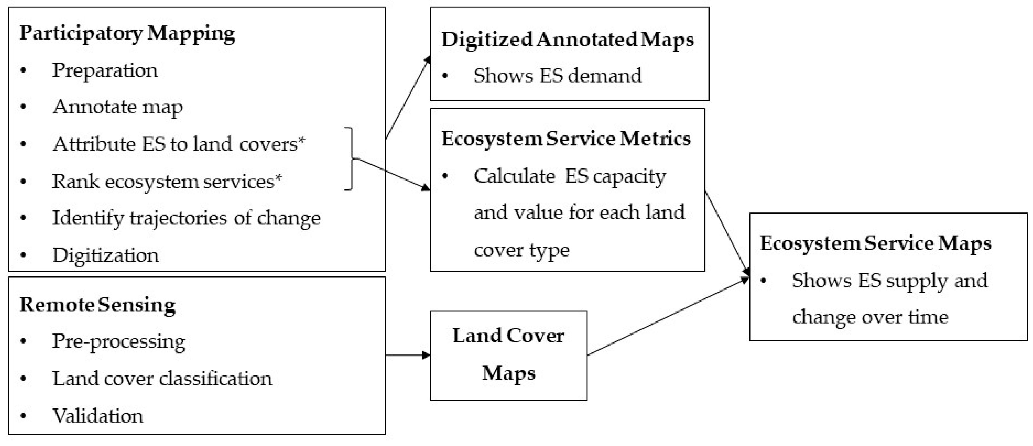
2.2. Participatory Mapping

In order to understand how environmental change has affected ES from the local perspective, and what these changes have meant for livelihoods, we carried out qualitative participatory mapping activities and focus group discussions in three communities (each a kebele, the smallest administrative unit of Ethiopia) in July 2018:

• Kopriay—historically more reliant on pastoralism with larger cattle herds, N = 1,094, 217 households;
• Ayepa—historically more reliant on flood-retreat agriculture, N = 1,275, 241 households;
• Napasmuria—largely poor households who have been subject to the wider regional conflict, generally resulting in their loss of animals and resettlement in a more urban context, and higher dependency on state resources such as safety net programs, N = 2,110, 418 households [63].

Whilst varying population estimates exist, these population numbers above are from the 2018 Livestock and Fisheries figures, and are the highest total population figures we found, suggesting the most ‘up to date’ estimate [63]. Village leaders from each community selected a group of adult men (n = 10) and adult women (n = 10) to participate in focus group activities, with the expectation of two three-hour meetings. This size of group represented the optimal size of volunteer focus groups as established in other participatory mapping studies [64,65]. Following norms in the literature [64,65], we split the focus groups by gender to ensure freedom of expression, to avoid gender bias in interpreting access to resources, and to see whether the men and women perceived change in ES differently. We worked with research assistants from the Nyangatom community, all male and university-educated, familiar with the area, with no bias or positionality detected. Michigan State University’s Institutional Review Board reviewed and approved all methods and procedures used in this research (MSU Study ID STUDY00000928, 05/29/18), determining the project to be exempt under 45. CFR 46.101(b) 2. In all instances, participants had to verbally consent to participate in the study before data collection commenced using an IRB-approved verbal consent process due to potential participant illiteracy. The participatory mapping has five main phases, outlined below and in Figure 2.

Preparation: A large A2 size print of a satellite image was used as a base map for the participatory mapping activities. A true-color composite image was created using the red, green and blue bands of the Sentinel-2 satellite which have a 10 m spatial resolution. The map extent covered the kebele and surrounding areas (~180–320 km²). A broad-scale map was also used to help situate the maps in relation to the wider Nyangatom woreda. The local kebele satellite maps were covered with a sheet of acetate and placed in the center of the participants of each community, oriented to true north, and different colored markers were provided. An explanation was provided, stating that the map shows the environment of Nyangatom, with the environment being the natural world. This includes nature, people, plants, animals, water, and all living things. Participants were first oriented in the satellite image by discussion of common landmarks (most commonly the river, roads, and settlements), to ensure participants could identify these and other landmarks on the map, were confident in the scale, and understood the orientation of the map. We also ensured that the research assistant was confident in interpreting the map so that they could spot if participants were misinterpreting the locations.

Annotate map: Participants were then asked, first in English and then in Nyangatom through the research assistant, to identify areas where they commonly used natural resources, whilst also explaining that as a group activity, a consensus (>50% agreement) must be reached to annotate the map. The terminology of “natural resources” was used as “ecosystem services”, which was not a familiar term to the community. The resources were analyzed via an ES lens by the research team. The same research team (authors 1 & 2 and research assistant) facilitated all focus groups. The facilitators ensured that different colors and patterns were used to annotate the map for different ES, and kept the legend updated. After an initial period of unconstrained conversation over the map and relative areal usages (30 minutes), participants were probed to discuss provisioning ES from forests, cropland, grazing land, and water sources, in order to fully explore change in these services as per norms in the literature [28,29], but also given the high levels of anticipated change highlighted in [46] (and summarized in Section 1) and the significant impact this was likely to have on livelihoods and food security. As asking about “natural resources” may bias the mapping towards provisioning ES, we then used Table S1 (see discussion below) to specifically probe for regulating and cultural ES, such as places of high biodiversity, spiritual sites, or community amenities (e.g., for education or recreation).

Attribute ES to land covers: As additions were made to the map, the research team annotated a pre-determined table of ES we would expect to find in this region (informed by the Millennium Ecosystem Assessment (MEA) [66], prior research and transect walks—see Table S1 in the supplementary material). Our intention was that participatory mapping would address all three categories of ES, as per the MEA. In the MEA the balance of ES is not even; for example, only 38 of the 344 indicators correspond to cultural ES, of which 32 focus on recreation and tourism [67]. Whilst we found a relatively diverse number of cultural ES in Nyangatom from our prior research and transect walks, in Table S1 there is still an uneven distribution amongst the three categories: 31 provisioning, 24 cultural, 18 regulating. For each addition to the map, focus groups were asked to identify on what land covers the service was found: bare ground, grassland, shrubland, forest, river, rain-fed ponds, river flood-fed lakes, urban, cropland. For the land covers identified, the group was then asked to rank the capacity of each cover category to provide the ES. For example, the female focus-group of Kopriay identified dryland grazing for cattle as being of high importance, and that it was provided by grassland and shrubland (joint first in capacity for its provision) and ponds (ranked second). During the map creation, notes were taken by the research team in English with assistance from the research assistant related to disagreements or consensus on boundaries, features, importance, or capacity. This process lasted about two hours for each group.

Rank ecosystem services: We presented each focus group with 10 tiles, each with a different graphic representing the most common provisioning ES (fish; honey; timber, fuel, and fiber (TFF); shade; grazing livestock; crops; water; wild fruits; bush meat; salt). Only provisioning ES were included as these were the most frequently mentioned ES in the participatory mapping that could be feasibly mapped with satellite remote sensing, as they most readily corresponded to particular land cover types (see Section 3.1.2). Groups were asked to rank the services (for the current day) by arranging the tiles from most important to least important and to explain the ranking. Again, the consensus had to be reached by the group (>50% agreement). This process lasted about 20 minutes.

Identify trajectories of change: An additional acetate sheet was then laid over the map, colored dot stickers placed nearby, and participants prompted to discuss the trends of the supply over the last five years, i.e., since 2013 in the Gregorian calendar, before the filling of the Gibe III reservoir began. Ethiopia has a distinct calendar based on the Egyptian lunar calendar. We clarified all participants were working from the same calendar during data collection and in our scoping work we identified other well-known events that occurred that year and used the Nyangatom name for those events to orient our participants in 2013. For each service annotated onto the map, the group had to decide whether it had increased (placing a green dot), stayed the same (placing a yellow dot), or decreased (placing a red dot), explaining to the facilitator whether this difference is because of environmental reasons or social reasons (i.e., a change in availability or access). This process allowed us to investigate whether the same ES were affected differently in the different geographic locations identified. Finally, participants were asked to identify the three increasing and three decreasing ES that will have the most impact on their lives, and to discuss why. If not already discussed, additional questions were asked to do with changing fodder availability, the productivity of crops, and which types of cultivation were most productive at both time points (2013 and 2018), ensuring that we left the focus group with an understanding of the multiple sources of food for each group, and whether they differed by gender. This evaluation of change process lasted approximately an hour.

Digitization: Following participatory mapping activities, digital maps of all features were created across four maps: agriculture, grazing, natural products, and cultural ES. Our digital participatory maps were made from combining features from all focus groups. Where communities referred to specific locations, (e.g., that of lakes, ponds, meeting places), discretion was used to move such points to their intended location following ground-truthing. Where multiple focus groups provided differing locations for specific landforms (e.g., grazing territories), the broader locations were used in the combined digitization of the feature. Figure 3 and 4 show the original map from one of the focus groups, and the digitized agricultural ES map compiled from all focus groups, respectively (Figure 4 can be found in the results section; the remaining digitized maps can be found in the supplementary material (Figures S1–S3)).

2.3. Remote Sensing

Figure 2 also gives an overview of the land cover mapping process. The Google Earth Engine cloud-based geoprocessing platform (https://earthengine.google.com/) [68] was used to generate land cover maps for two time periods: 2000–2003 (using Landsat 7’s Enhanced Thematic Mapper) [69] and 2016–2019 (using Landsat 8’s Operational Land Imager) [70].

Pre-processing: The orthorectified and atmospherically corrected Tier 1 Surface Reflectance products were used [71]. Cloud and cloud shadow were masked from the imagery using the Quality Assurance (QA) bands. For each time period, a median value composite and greenest pixel composite were produced. The greenest pixel composite was generated by selecting pixels with the maximum Normalized Difference Vegetation Index (NDVI) value during the period. The spectral bands (1–5 and 7 for Landsat 7 and 2–7 for Landsat 8) for both the median and greenest pixel composites were combined into a single image.

Land cover classification: Unsupervised classification was then performed using k means clustering, with the number of clusters set to 100. The 100 spectral clusters identified were each assigned to one of six land cover classes based on visual interpretation of the imagery, in addition to interpretation of historic high-resolution imagery from DigitalGlobe QuickBird, and WorldView-1 and 2 within Google Earth (consistent with various remote sensing studies, e.g., [72,73]). The land cover classes were water, wetlands, bare ground, grassland, shrubland, and forest (see Table S2 and Figure S4 in the supplementary material). The land cover classes that could be spectrally separated in satellite imagery did not directly correspond to the classes identified by the communities. Despite its importance, cropland could not be mapped due to the difficulty separating it from other classes such as grassland, shrubland and bare ground. Cropland is challenging to map as it is spectrally similar to other land cover types, particularly small plots for subsistence farming which can be smaller than pixel sizes [74]. Urban areas (i.e., villages, schools, Kangaten town) were included as part of the bare ground class as these classes were also difficult to separate. Both urban and bare ground provided no provisioning ES with the exception of poultry, which was not included in the mapping as it was associated with a landscape feature—i.e., villages—rather than a land cover. Finally, the river, ponds, and lakes could not be separated based on their spectral signatures in the satellite imagery. However, since these land covers had different significance to communities (lakes were previously refilled by the Omo flood and thus provided different services to ponds which were further from the river and filled by rainwater), an alternative method for separating these classes was applied where the river, lakes and ponds were separated by dividing the study area into different zones, including: (i) River Zone: the main river channel, (ii) Lake Zone: low-lying land close to the river, and (iii) Pond Zone: the remaining area. The water and wetland land cover types were then classed as river, lakes and ponds depending on which of these zones they were located in. The River Zone was generated using the JRC Global Surface Water product to identify areas with a water occurrence of > 25% over the period 1984–2015, which were then converted to a vector file. The river polygon was selected and a buffer of 120m was added. The pond and lake zones were separated using the WWF HydroSHEDS Hydrologically Conditioned Digital Elevation Model (DEM), with 3 Arc-Second spatial resolution. The Lake Zone was defined as areas with an elevation less than 405 m.

Validation: Land cover maps were validated using ground data points recorded in the field in July 2018 using the SW Maps App [75] on Android devices with built-in GPSs. Ground data were collected both on foot, during transect walks and community visits, and from vehicles during travel between communities and to specific sites mentioned by focus groups. Following fieldwork, ground data were quality controlled and ‘cleaned’ to move points off roads using ArcGIS software and high-resolution imagery. Due to difficulties collecting sufficient water and wetland points in the field, additional randomly distributed ‘ground-truth’ points were generated for these classes using ArcMap and visual interpretation of high-resolution imagery. In total, 702 validation points were used, 389 of which were added retrospectively mainly for the water, forest and wetland categories. The 2016–2019 map was validated using the full dataset while the 2000–2003 map was validated using only points that had remained unchanged and had the same land cover type in both maps. Accuracy matrices were generated and the total accuracy and kappa coefficient for each map was calculated to assess the classification uncertainty (c.f., Tables S3 and S4 in the supplementary material).

2.4. Deriving ES Metrics for Each Land Cover Type

Data from the ranking activities in the focus groups was used to calculate ES metrics for each land cover class, including the number of services, number of service categories, ES capacity (i.e., the ability of the land cover to support the given ES), and ES value (i.e., the human-derived value of the ES supported by the land cover). These metrics were calculated for provisioning ES only, as these are the services that were most frequently mentioned during the participatory mapping and which most readily corresponded to land cover classes (see Section 3.1.2 for further explanation). Responses from men’s and women’s focus groups were merged to produce a single capacity matrix for each community. This was done to account for the different gender roles between men and women which might restrict both groups from being able to comment on all services. For example, when women in some communities were asked about fish, they said that we should speak to the men because they do the fishing. Similarly, women could provide more information on fuelwood and building materials, while men appeared to know more about grazing. Where only one gender reported ES capacities these values were used; when both genders provided data the mean capacity scores were used.

Individual ES reported by communities were grouped into service categories (Fish; Honey; TFF; Shade; Livestock; Crops; Water; Wild fruits and Bush meat) to enable integration with the importance rankings that were used as weightings for calculating ES value. The number of services and number of ES categories provided by each land cover type was determined from the capacity matrix for each community. The service-specific capacities—i.e., the capacity of the land cover type x to provide service y—were aggregated by summing up the capacity scores for all individual services in each ES category to give an ES category-specific capacity.

The total ES Capacity, C_i, of the i^th land cover type was then calculated as the sum of the ES category-specific capacities, c_i,n, for each land cover type:

$$C_i= {\displaystyle \sum }_{n=1}^{n=N}{c}_{i,n}$$

(1)

where $c_{i,n}$ is the capacity of land cover type i to provide service category n, and N is the number of ES categories. Lastly, the ES value of the i^th land cover type, $V_i$ is given by:

$$V_i= {\displaystyle \sum }_{n=1}^{n=N}{c}_{i,n}{I}_n$$

(2)

where $I_n$ is the mean importance of service category n to the communities, as determined in the importance ranking activity.

2.5. Integrating Traditional Ecological Knowledge with Satellite Data to Map Ecosystem Services

ES maps were derived by integrating the land cover maps produced with information about the ES capacity and value of each land cover type obtained from the focus groups. The total ES capacity and value scores of each pixel was assigned based on the land cover type. ES capacity and value maps for both time periods were generated. Maps showing the change in ES were also generated by calculating the change in ES capacity and ES value between the two periods. The change in ES for each kebele was then additionally calculated.

3. Results

3.1. Participatory Mapping

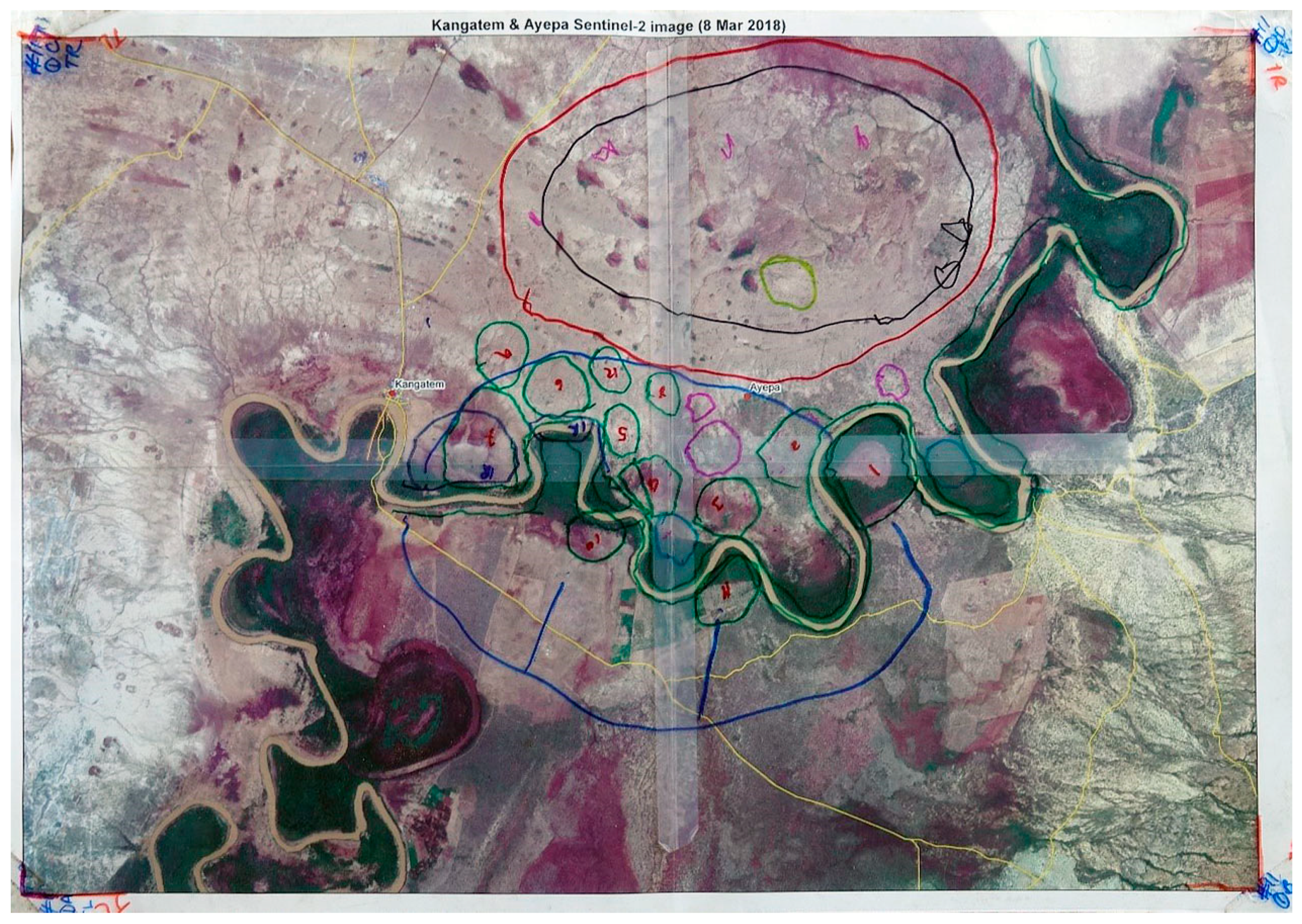
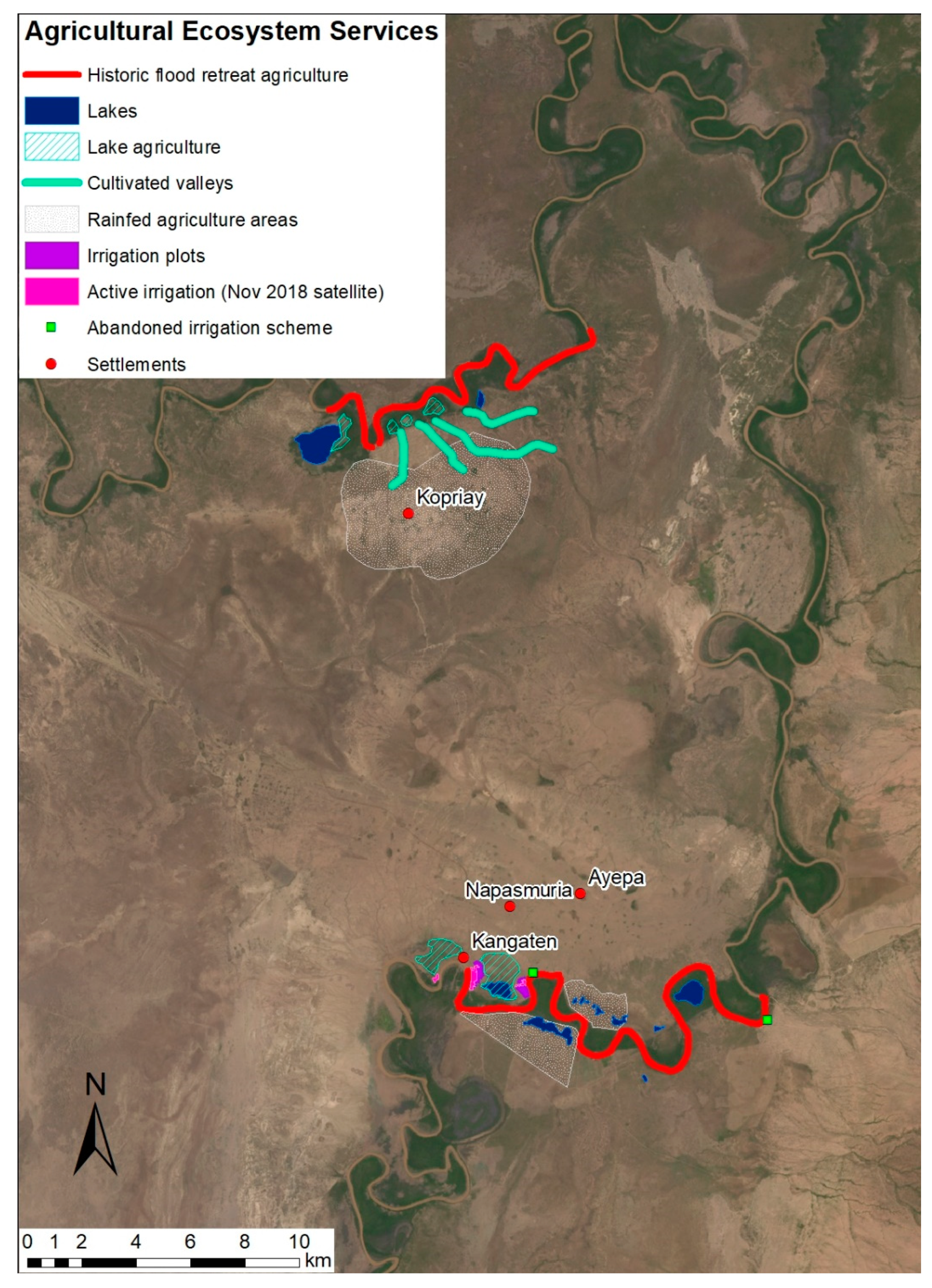
3.1.1. Annotated Maps

Features mapped by each community were digitized and split into four categories: arable agriculture, grazing, natural products, and cultural. The digitized map for arable agriculture ES is included as an example (Figure 4) and the other maps are available in the supplementary materials (Figures S1–S3). The rest of this section describes insights gained from the annotated maps.

Landscape features and natural resources that were added to the map by participants first were, unsurprisingly, related to livelihoods, from which we could elicit key provisioning ES, i.e., dry and wet season grazing and subsistence crop production. Groups drew multiple sites for cultivation onto the maps, which differed by the source of water but generally produced the same subsistence crops (sorghum, maize, cow peas, pumpkin, watermelon, tobacco, calabash). Five main cultivation types were defined and are shown on Figure 4:

• Flood retreat agriculture (red on Figure 4): cultivation in the rich silt left along the river banks as the flood recedes [56,76], no longer available as there have been no floods since 2016. As one female participation said, “we don’t talk about the Omo, because the Omo is no more”.
• Lake cultivation (hatched turquoise areas on Figure 4): at peak flood, the Omo River would fill large bodies of water between meanders of the river, in which cultivation would be carried out as it receded. Participants relayed that due to the loss of the flood, these are now only rainfed, but still defined as lakes by the community, in contrast to:
• Pond cultivation (grey-dotted areas on Figure 4): temporary rain-fed ponds that form during the wet-season, in which cultivation is carried out as it receded.
• Valley cultivation (turquoise lines on Figure 4): between Kopriay and the river there are valleys that can be cultivated during the wet season.
• Irrigation (pink areas on Figure 4): some irrigation is supported by the woreda near Kangaten, currently for cultivation of grass for fodder programs. The green dots represent historic irrigation sites, established by the Swedish Philadelphia Church Mission (SPCM) and active between the early 1970s until the early 2000s.

There is some overlap between rain-fed cultivation and grazing. The rain-fed ponds, and now lakes, also support the growth of grass on which livestock are also grazed, as shown in Figure S1. Herds consist of cattle, sheep, and goats. During the wet season, all types of livestock graze close to the communities, including nearby ponds. Sheep and goats remain around the communities year-round, and utilize the dry season grazing nearest to the communities. Dry season grazing lands for cattle extended beyond the extent of the kebele maps, as livestock are herded into Nyangatom territory dozens of miles further west. Other provisioning services are shown in Figure S2, which synthesizes non-agricultural ES, including:

• Fishing, in the river and large lakes. Fishing in the river was traditionally a man’s task, with fish often consumed at the river immediately. According to an Ayepa woman “Why are you asking us about the fish? It’s the men’s work… Most of the time, we women do not eat the fish. Fish is for men. They eat there and if they like it they sell it there. If they wish to bring home, it’s according to their will; it’s not a must.”
• Hunting and trapping. Again, a gendered activity, with men hunting larger animals, often for cultural reasons as well as for food. Women and children trap smaller animals nearer to their settlements.
• Wild fruits, collected in the shrubland and forests around Ayepa and Napasmuria.
• Timber, fuel, and fiber, collected in the riverine forests.
• Water for livestock, accessed at ponds and lakes. The grazing ES map (Figure S1 in the supplementary material) also shows some waterholes for livestock by the river.
• Amokat, a salty soil, mixed with tobacco as a flavor enhancer and smoked.

Whilst not reported on the map, drinking water for communities was reported as a service in the focus group discussion. Participants reported using both the river, lakes, and ponds at different times of the year, but did not annotate it on the map as the areas were already highlighted for other services.

The mapping activity aimed to cover all three categories of ES. Given our prior work and Table S1 including more provisioning ES than cultural or regulating, the balance of mapped ES was anticipated. Common cultural ES that were included on the map (Figure S3 in the supplementary material) included ceremonial and dancing sites, however, many of the cultural ES discussed (both freely brought up and probed) did not have a specific location (i.e., places of beauty, places of inspiration, places for recreation, places for hunting for ceremonial wear) or were difficult for the community to map because they had such a specific location (i.e., an individual tree where people met to talk or resolve conflict). During the mapping, the community also listed churches, schools, and clinics, which whilst not ES (although some schools are not in physical buildings but in specific environmental spaces, e.g., under a known tree) are shown as well. Regulating services were the least discussed, although we can assume certain regulating services from conversations about pest extent and water quality throughout the region. These however were not mapped, but again, this does not mean that the Nyangatom did not value these ES. Overall, Kopriay mapped the smallest diversity of ES, and Ayepa the most. Generally, women identified more provisioning and regulating services whilst men identified more cultural services. For further detail please see Table S5.

3.1.2. Attribute Ecosystem Services to Land Covers and Rank Ecosystem Services

During mapping, the participants identified which ecosystem services were found in which land covers and ranked the land covers for their capacity to provide that service. After mapping, the provisioning services that were mapped most frequently were presented to the participants on tiles. As mentioned in Section 2.2 and Section 2.4, only provisioning ES were ranked as cultural services tended to be associated with specific landscape features (e.g., an individual tree) rather than broad land cover types (see Figure S3), meaning they could not be readily mapped using satellite land cover data. Whilst regulating ES are often mapped with RS-GIS, given they were not commonly included in the participatory mapping (see Table S5), we did not include them in the ranking activity. The results presented here therefore integrate the two sections from the methodology of ‘Attribute ecosystem services to land covers’ and ‘Rank ecosystem services’. Further detail on the importance and capacity data is presented in Section 3.3 on ES metrics.

Table 1. Rankings of tiles that represented the top 10 provisioning ecosystem services (TFF = Timber, Fuel, and Fiber, K = Kopriay, A = Ayepa, N = Napasmuria, W = Women, M = Men). Tiles ranked 1st were given 10 points, through to the 10th rank given 1 point. The table is ordered according to the mean score.

Community	Water	Crops	Grazing Livestock	Wild Fruits	Fish	TFF	Bush Meat	Shade	Salt	Honey
K-W	8	9	10	7	5	2	6	1	3	4
K-M	10	8	9	6	2	3	1	7	5	4
A-W	10	10	10	4	5	7	1	2	6	3
A-M	10	9	8	7	4	5	6	3	2	1
N-W	10	10	8	3	5	6	4	7	2	1
N-M	10	9	8	7	6	2	5	3	1	4
Mean	9.7	9.2	8.8	5.7	4.5	4.2	3.8	3.8	3.2	2.8
SD	0.8	0.8	1	1.8	1.4	2.1	2.3	2.6	1.9	1.5
Mean (W)	9.3	9.7	9.3	4.7	5.0	5.0	3.7	3.3	3.7	2.7
Mean (M)	10.0	8.7	8.3	6.7	4.0	3.3	4.0	4.3	2.7	3.0

displays the results of the tile ranking activity.

The results of the ranking demonstrate that grazing livestock, subsistence crops, and drinking water are the highest ranked. Water was frequently ranked first because of its role in providing all other services, as a female participant from Kopriay explained via translation:

“Water is life…. Water is also future. The animals also drink water. The grains also use water. The wild food/fruit also use water. The sun also needs water. When the rain rains, the sun comes out. The bees also drink water, that’s why it is producing the honey. The materials for building house and firewood, even they require water. The fish is also drinking water and taking shower in the water. Wildlife also use water for drinking. The cattle also drink water. After drinking water, they produce milk and butter and meat, produce skin for sleeping.”

Contrastingly, bush meat, honey, salt, and shade have the lowest mean scores in the ranking activity. However, this varied by community and, as reflecting in the rankings, in Napasmuria, honey and fish were more important. In other communities, when honey was ranked lowly, it was because of its seasonal nature:

“Because honey is not available at every time. Also, honey cannot be eaten like food. You have to eat it slowly with other foods.” [Ayepa man].

Contrastingly, when ranked more highly it was because of its use as a trading product or for special foods:

“Honey is used to sell and buy cattle and goats. Honey is also used for alcohol.” [Kopriay woman].

Wild fruits, fish, and TFF were the most varied in their rankings. Fish was ranked by women consistently as fifth most important, but there was more variation in the male participants, which matches the extent to which a community seems to be utilizing fishing and the gendered nature of it, as a male activity. The Napasmuria men are fishing more than the Kopriay men, and rank it accordingly. Table 1 shows that hunting and trapping bush meat was less popular than fishing or wild fruits, however, rather than reflect the seasonal nature of this as a service, as per honey, this is conceivably because of the lack of animals for hunting in close proximity to the communities. The terminology of wild fruits, as used in the communities, is a little limiting; it refers to both food from the trees and from below the ground (i.e., potato-like species). Women had a higher ranking of crops and men of wild fruits. The latter is interesting given that traditionally women collect wild fruits, not men, but this may reflect the higher dependence on this service than in the past, expanded on below, and therefore the greater consumption by men at the moment than at other periods in time.

3.1.3. Identify Trajectories of Change

After the present-day conditions were mapped in the focus groups, the trajectory of change was marked for each ecosystem service added to their map. Not every group mapped every ecosystem service, as

Table 2. Reported trajectories of change from the mapping activity, condensed to the most commonly mapped ecosystem services - ⇘ indicates decrease, ⇗ indicates increase, ⇔ indicates no change, and a blank space indicates the service wasn’t reported. The final column is the general reported direction of change in the region (K = Kopriay, A = Ayepa, N = Napasmuria, W = Women, M = Men).

Ecosystem Service	K-W	K-M	A-W	A-M	N-W	N-M	Overall
Grazingfodder	⇘	⇘	⇗	⇘	⇘	⇘	⇘
Grazing—number of livestock supported	⇗	⇗		⇘		⇗	⇗
Drinking water—livestock	⇘	⇘		⇘			⇘
Drinking water—humans			⇔	⇘			⇘
Salt	⇘	⇘					⇘
Cultivation—flood	⇘	⇘	⇘	⇘	⇘	⇘	⇘
Cultivation—lake	⇘	⇘	⇘	⇘	⇘	⇘	⇘
Cultivation—rainfed	⇘	⇘	⇘	⇘	⇘	⇘	⇘
Cultivation—Irrigation			⇘	⇘	⇘	⇘	⇘
Wild fruits	⇘	⇘	⇗	⇘	⇘	⇘	⇘
Bush meat	⇘	⇘				⇘	⇘
Timber, Fuel, and Fiber			⇘		⇘		⇘
Honey				⇘			⇘
Fishing		⇘			⇘	⇘	⇘
Schools	⇗		⇗	⇗	⇔	⇗	⇗
Ceremonial sites	⇘	⇗	⇗	⇗	⇘	⇔	⇗
Villages		⇗			⇗	⇗	⇗

shows. Table 2 also presents the reported direction of change (>50% consensus in the group) for each group, as well as the overall direction of change in the region since 2013, i.e., before filling of the Gibe III reservoir began.

Very few services had remained static, and overall, provisioning ES were reported to be decreasing (Table 2). Generally, participants reported a decrease in fodder availability. In Kopriay and Napasmuria, participants attributed this to increased livestock numbers, although for different reasons—due to vaccination programs in Kopriay, but in Napasmuria due to grazing by outsider’s livestock, particularly large numbers of donkeys, presumed to be from Kangaten. Some difference was exhibited in Ayepa where women reported an increase in grazing, but men reported a reduction in livestock numbers given disease and no corresponding increase in fodder—in fact, the opposite. We interpret this to mean an increase in access to grazing land, and therefore fodder, for the women, but not necessarily an increase in output. The increase in Napasmuria is not likely to be cattle; as resettled households, they have a higher proportion of female-headed households and thus sheep and goats are common.

Table 2 also reports outputs from cultivation, and for flood-retreat cultivation all communities reported a decrease. The decrease was often phrased as a collapse due to the rapid decrease in area under cultivation given the greatly reduced hydrological fluctuations of the Omo. Similarly, outputs were reported to have decreased from lake cultivation, as it was also previously supported by the seasonal flood and consequently cultivated area here also decreased. Rainfed cultivation had increased in area (around ponds and in valleys), but that had not resulted in increased outputs. Droughts in recent years may explain the differing perceptions of its availability. Ayepa and Napasmuria reported that the irrigated land they had access to had also decreased, as pumps had broken and were not fixed, resulting in low and decreasing outputs.

The services that communities turned to next - fishing, wild fruits, and bushmeat - were all reported to be decreasing, for both supply and demand reasons. The Napasmuria participants reported less fish in the lakes, attributed by participants to be due to the loss of the annual flood which enabled migration of fish and transfer of water into them. Participants from all three communities reported that the lack of rain in the past few years had diminished the supply of wild fruits, but also that more people and animals were collecting them, resulting in less per person. Similarly, decreases in wood for both fuel and building materials were attributed to increased competition, resulting in women having to travel increasingly farther distances.

It seems that the increasing competition is not solely because of the decrease in natural resource availability, but also because of increasing populations. The numbers of villages were reported to have increased in Kopriay (owing to growth of the existing population) and Napasmuria (from immigration). This growth led to the creation of more ceremonial sites but was not constant across all three communities as conversion to Christianity reduced the use of such areas, i.e., in Napasmuria.

The reporting of these services was explored in more detail by asking the groups to rank the top three most important increasing and decreasing services, shown in

Table 3. Participants ranked the ecosystem services that were reported to have changed since 2013 according to their perception of importance of this change, this table presents the three highest ranked for both increasing and decreasing ecosystem services (K = Kopriay, A = Ayepa, N = Napasmuria, W = Women, M = Men; 1 = highest ranked, 2 = ranked second, 3 = ranked third).

	K-W	K-M	A-W	A-M	N W	N-M
Increasing 1	Schools	People	Schools	Ceremonial sites	Schools	Donkeys
Increasing 2	Cattle numbers	Cattle numbers	Ceremonial sites	Schools	Sheep & goat numbers	Pond cultivation
Increasing 3	Salt	Villages	Grazing	n/a	Pond cultivation	Villages
Decreasing 1	River cultivation	River cultivation	River cultivation	River cultivation	River cultivation	River cultivation
Decreasing 2	Bush meat	Lake cultivation	Lake cultivation	Cattle	Irrigation	Irrigation
Decreasing 3	Grazing/ water	Grazing	Pond cultivation	Grazing	Lake cultivation	Lake cultivation

. Its contents reflect the synthesis above; that whilst population and cultural ES are increasing, there are trade-offs with provisioning services in addition to changes in supply due to the hydrological changes.

Table 3 shows that within the existing and new villages, schools are being constructed—this is as part of the Productive Safety Nets Program [77,78]. Whilst not an ecosystem service (hence in italics in Table 3, although some still exist in particular locations valued for their shade, not in a structure), these are of high importance to the communities, who were glad that formal educational opportunities were increasing—in contrast to prevailing opinions in other ethnic groups in Ethiopia that pastoralists do not recognize the value or prioritize education for their youth [79]. The Ayepa men were particularly keen to stress that formal education was a critical part of what would help most in the future:

“We need pumps for irrigation, taps for drinking water, food, as well as new school construction”.

With respect to the provisioning ES, Table 3 reiterates some of the findings of Table 2 in that livestock numbers are increasing in Kopriay and Napasmuria (although for different species)—that the loss of the flood and river cultivation has been the service whose decreasing provision has had the greatest impact, and that the substitutes for river cultivation are also decreasing, rather than increasing to match the need. We explore that further in the next section.

3.1.4. Changing Cultivation

Given the reported importance of the loss of flood-retreat cultivation by the river, we asked further questions about how each community had adapted, i.e., what sources of cultivation have now become the most productive and important?

Table 4. Cultivation practices before (2013) and after (2018) Gibe III dam construction and thus after the annual flood ceased.

Community	2013	2018
K-W	River > Lake > Valley	Valleys > Lake
K-M	River > Lake > Valley > Ponds	Lake > Valley > Ponds
A-W	River > Lake > Irrigation > Pond	Pond > Irrigation > Lake
A-M	River > Irrigation > Pond > Lake	Pond > Lake > Irrigation
N-W	River > Lake > Irrigation > Pond	Lake > Pond > Irrigation
N-M	River > Lake > Irrigation > Pond	Pond > Lake > Irrigation

summarizes these results.

Table 4 shows that most communities have coped with the loss of flood-retreat agriculture by relying more on rainfed agriculture, either in ponds (all communities), lakes (now rainfed not fed by the seasonal flood; all communities), or valleys (Kopriay only). Ayepa and Napasmuria have some access to irrigation, but it is not consistent throughout their populations. While these communities have been provided with several diesel-powered pumps for irrigation, only one pump was operational at the time of our field work. The pump was being used to irrigate grass for fodder rather than for crop cultivation. The government has promised more pumps, though such provisions have in the past suffered from problems of inadequate mainte nance, lack of fuel and reported theft of parts.

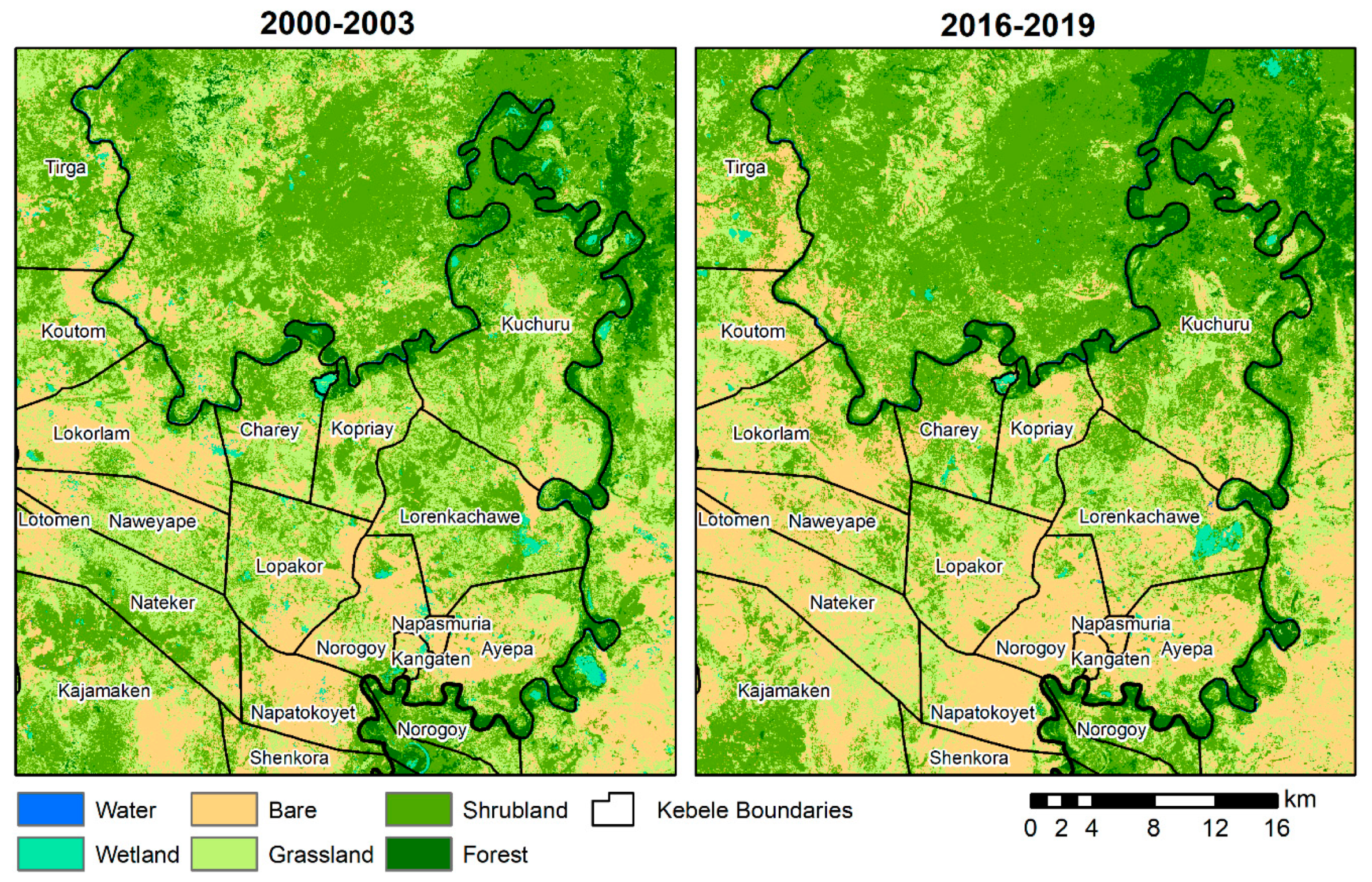
3.2. Land Cover Mapping

Land cover maps for 2000–2003 and 2016–2019 are shown in Figure 5. The maps had a high accuracy when compared against our validation dataset (2000–2003 map: overall accuracy = 89.9%, kappa = 0.874; 2016–2019 map: overall accuracy = 94.3%, kappa = 0.924). Accuracy matrices for the maps can be found in Table S3 and Table S4 in the supplementary materials. Most notably, there has been a large increase in bare ground between the two periods generally owing to a reduction in grassland and shrubland, also shown in

Table 5. Change in area (hectares and percentage change) of each land cover type between 2000–2003 and 2016–2019 in Nyangatom kebeles. P = permanent, S = seasonal.

	River				Lakes				Ponds				Bare Ground		Grassland		Shrubland		Forest
	P		S		P		S		P		S
Kebele	ha	%	ha	%	ha	%	ha	%	ha	%	ha	%	ha	%	ha	%	ha	%	ha	%
Ayepa	3.9	53	−42.6	−72	NA	NA	−3.9	−17	0	0	−1.6	−4	778.3	30	−496.9	−21	−337.6	−18	100.3	15
Charey	6	55	−7.2	−52	NA	NA	−29.1	−98	NA	NA	−16.8	−24	284.8	36	−766.1	−33	615	33	−85.8	−21
Kangaten	NA	NA	NA	NA	NA	NA	−41	−98	NA	NA	NA	NA	179.8	61	−110	−75	−28.7	−75	NA	NA
Kopriay	1.6	62	−3.2	−60	NA	NA	−8.6	−88	NA	NA	2.4	21	526.5	52	−206.9	−10	−305.9	−21	−6	−2
Kuchuru	16.5	91	−68.4	−62	−0.8	−82	−109.6	−98	NA	NA	−17	−95	491	28	−1737.7	−28	1040.4	12	385.3	13
Lokawamunyen	NA	NA	NA	NA	NA	NA	NA	NA	NA	NA	0.4	200	20.7	7	−18.5	−32	−4.3	−24	NA	NA
Lopakor	NA	NA	NA	NA	NA	NA	NA	NA	-0.4	−57	−101	−99	689.9	29	−277.4	−9	−315.3	−20	4.2	62
Lorenkachawe	2	70	−8.3	−67	−5	−52	196.6	113	NA	NA	−28.5	−62	1672.3	131	−231.2	−5	−1632.9	−39	34.7	26
Napasmuria	NA	NA	NA	NA	NA	NA	−15.5	−85	NA	NA	−1.9	−91	60.2	19	−47.4	−61	3.8	28	0.7	800
Napatokoyet	12	122	−28.3	−84	−0.9	−83	−90.8	−93	NA	NA	NA	NA	462.1	16	336.2	22	−507.8	−26	−178.1	−35
Naweyape	NA	NA	NA	NA	NA	NA	NA	NA	NA	NA	−29	−87	1270	71	−1134.3	−43	−93.7	−9	−13.1	−91
Norogoy	11.6	126	−31.7	−71	NA	NA	−41.2	−94	−0.9	−34	−47.6	−66	1049.6	42	−554.4	−27	−352.2	−17	−33.1	−8
Total	54		−189		−7		−143		−1		−242		7486		−5244		−1920		209

. Wetland areas also decreased substantially, and many of the river adjacent lakes that were previously refilled by the Omo River, before the Gibe III dam began regulating river flows, are now dry. The amount of forest has however remained approximately the same.

3.3. ES Metrics

The derived provisioning ES metrics for each land cover type are shown in

Table 6. Provisioning ecosystem service (ES) sub-categories supported, mean number of ES, number of ES sub-categories, ES capacity and ES value for each land cover type across the three communities, as determined by participatory mapping activities. TFF = Timber, Fuel and Fiber.

Land Cover	ES Sub-Categories Supporteda	Mean Number of ES	Mean Number of ES Sub-Categories	Mean ES Capacity	Mean ES Value
Shrubland	Livestock (3), Wild Fruits (3), Bushmeat (3), TFF (2), Crops (1), Honey (1), Shade (1)	9.33	4.67	0.95	0.83
Ponds	Water (3), Crops (3), Livestock (2), Shade (1), Wild Fruits (1), TFF (1), Honey (1), Bushmeat (1)	6.33	4.33	0.70	0.78
River	Fish (3), Water (3), Livestock (1), Bushmeat (1)	4.67	2.67	0.58	0.66
Lakes	Crops (3), Fish (2), Livestock (2), Wild Fruits (1), Water (1), Honey (1), Bushmeat (1), TFF (1)	5.67	4.00	0.61	0.65
Forest	Wild Fruits (3), Wood (3), Bushmeat (2), Honey (2), Livestock (1)	5.00	3.67	0.77	0.57
Grassland	Livestock (3), Crops (1), Bushmeat (1), TFF (1)	4.67	2.00	0.36	0.46
Cropland	Crops (3)	1.00	1.00	0.18	0.24
Bare ground and Urban	None	0	0	0	0

^a Brackets represent the number of communities that reported services in each ES category.

. Shrubland provided the most services and service sub-categories (including Livestock, Wild Fruits, Bushmeat, and TFF) and had the highest ES capacity and value. Ponds provided the second most services and service sub-categories (including Livestock, Water, and Crops), and had the second highest ES value (although forests had the second highest capacity). The high ES value of shrubland and ponds was not anticipated prior to participatory mapping with communities, highlighting the need to incorporate TEK into ES mapping for providing contextually relevant information.

The river provided relatively few service sub-categories and thus had a modest capacity score; however, its ES value was high due to water being the most important service sub-category (Table 1). Lakes had a relatively high ES capacity and value. Prior to the Gibe III dam, lakes are expected to have possessed higher capacity to provide services, likely higher than ponds, but the focus groups were concentrated on present capacities. Forest had the highest capacity to provide services, but its overall ES value was relatively low since many of the services sub-categories it provided were of lower importance to communities (see Table 1). Grassland and cropland provided few services, particularly cropland which only provided one service, resulting in their ES capacities being low. However, the services these land covers provide have high importance, boosting the ES value of these land covers. Bare ground and urban areas provided no services and thus had no ES capacity and value.

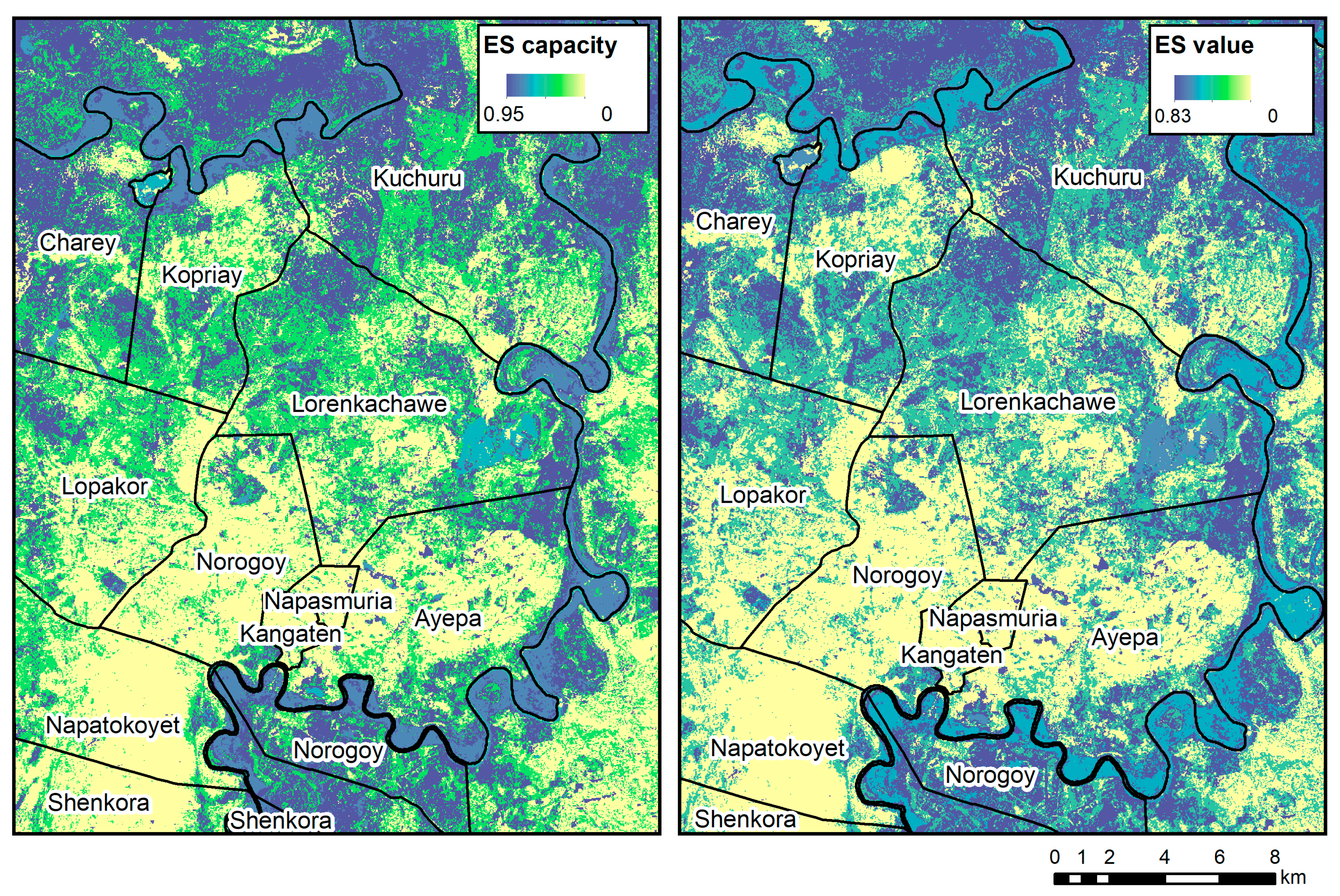
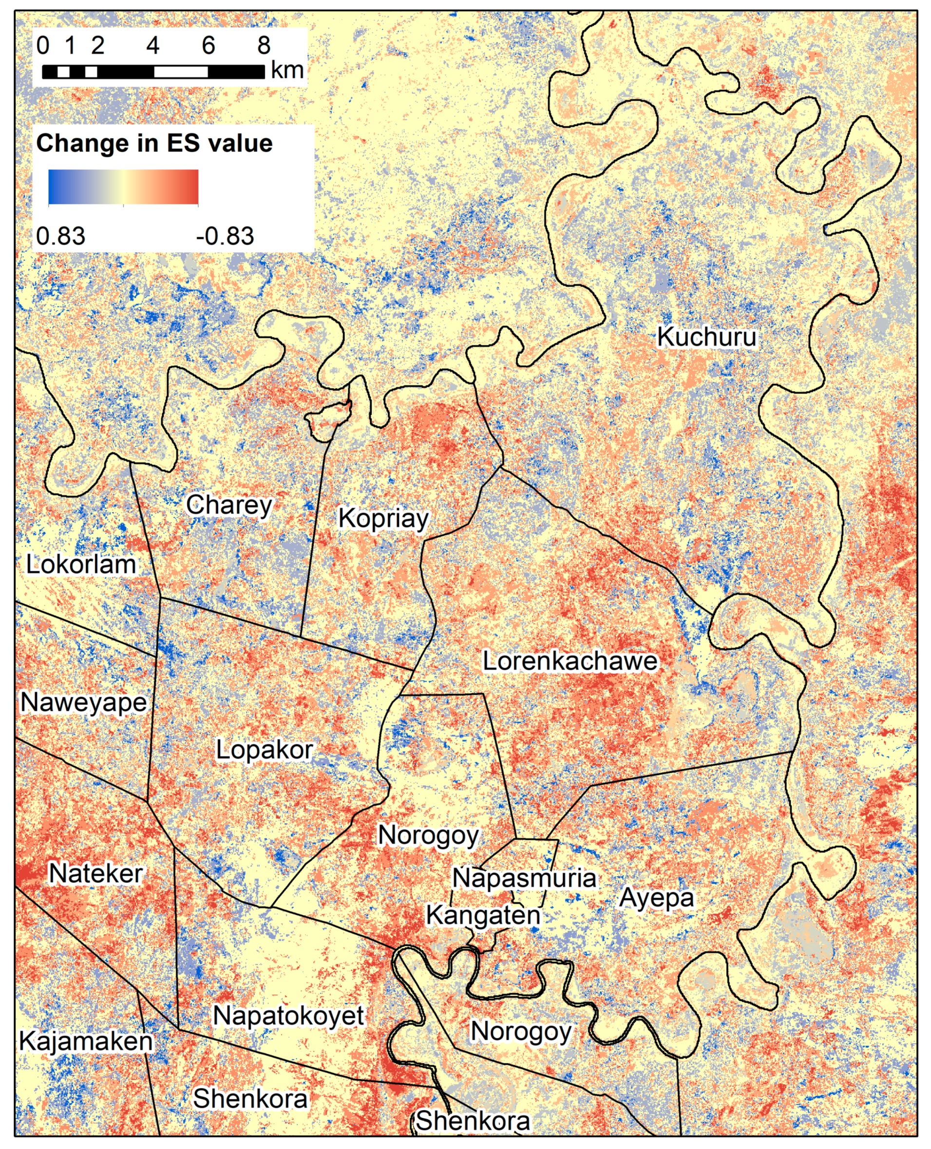
3.4. Integrated ES Maps

Maps of ES capacity and ES value for 2016–2019 for our focal communities and surrounding kebeles are shown in Figure 6. The two maps demonstrate broadly similar spatial patterns, with higher ES scores close to the river and in shrubland areas. The main difference between the maps is that grassland are colored green in the ES capacity map and turquoise in the overall value map due to the higher ES value score relative to its capacity (i.e., the services it supports are of proportionally greater value to communities than their ability to support those services). Additionally, forest appears a lighter shade of blue in the ES value map because it has a lower ES value score than capacity score.

The change in ES value between 2000–2003 and 2016–2019, for Omo River adjacent kebeles in Nyangatom, is shown in Figure 7. There are extensive dark red areas highlighting the overall decrease in ES value. This is largely due to a loss of shrubland, and to a lesser extent grassland, and an increase in bare ground (again, of no ES value). Interestingly, dark red areas in the northern part of Kopriay coincide with valleys that communities indicated as important areas for cultivation, particularly now flood retreat-cultivation along the Omo is no longer possible. These areas have likely been cleared of shrubland to grow crops. As our land cover classification did not include cropland these areas were classed as bare ground in the 2016–2019.

Our focal communities (Kopriay, Ayepa and Napasmuria) all showed a decrease across all ES metrics (

Table 7. Summary of provisioning Ecosystem Service (ES) metrics for kebeles in Nyangatom in 2000–2003 and 2016–2019, and the percentage change between these periods.

	Number of Services			No. of ES Sub-Categories			ES Capacity			ES Value
Kebele	00–03	16–19	% change	00–03	16–19	% change	00–03	16–19	% change	00–03	16–19	% change
Kopriay	5.20	4.30	−16	2.50	2.10	−16	0.49	0.41	−16	0.49	0.41	−15
Ayepa	4.30	3.60	−16	2.10	1.80	−14	0.42	0.36	−14	0.41	0.34	−15
Napasmuria	1.40	0.76	−46	0.70	0.36	−48	0.12	0.07	−44	0.14	0.07	−49
Kangaten	2.50	0.52	−79	1.20	0.24	−81	0.22	0.04	−80	0.24	0.05	−80
Charey	5.60	5.90	5	2.80	2.90	5.4	0.55	0.58	7	0.53	0.55	3
Lorenkachawe	6.00	4.50	−25	2.90	2.20	−25	0.57	0.42	−26	0.56	0.43	−24
Norogoy	4.50	3.50	−21	2.20	1.80	−21	0.44	0.35	−20	0.42	0.33	−21
Lopakor	4.10	3.50	−17	2.00	1.60	−18	0.37	0.31	−18	0.39	0.32	−17
Naweyape	4.00	2.80	−29	1.90	1.30	−28	0.35	0.26	−27	0.38	0.27	−30
Lokawamunyen	1.20	0.92	−26	0.57	0.43	−24	0.11	0.08	−24	0.12	0.09	−26
Napatokoyet	4.10	3.40	−16	2.10	1.70	−19	0.41	0.33	−19	0.39	0.32	−16
Kuchuru	6.30	6.40	2	3.20	3.30	3.4	0.64	0.67	4	0.60	0.60	1

). Of the three communities, Napasmuria had the lowest initial values and the largest percentage decreases. Kangaten kebele (which includes Kangaten town) also had low initial ES metric scores and showed the largest percentage decrease of all kebeles mapped, with a change in ES value of −80%. The remaining kebeles showed similar or slightly larger decreases than Kopriay and Ayepa, except for Charey and Kuchuru, which both showed a slight increase in ES scores. Interestingly, Kuchuru kebele is inhabited by the Kwegu ethnic group, whose livelihoods are based strongly on hunting, fishing and honey cultivation [80]. However, the Kwegu also practiced flood-retreat cultivation along the Omo [81,82] but do not generally keep livestock, which may explain the lack of ES degradation.

4. Discussion

The aim of this paper was to a) demonstrate an approach for combining participatory methods with remote sensing to provide a more holistic understanding of the dynamics of ES, and b) apply this in the Lower Omo Valley, Ethiopia, showing for the first time the ES impacts of regional developments for communities in the Omo River basin.

4.1. ES Change in the Lower Omo

By integrating Lower Omo users’ knowledge, perceptions, and experiences of ES at the local scale with satellite data, we have quantified ES change over time (describing both the spatial and temporal dynamics in ES) and validated community perceptions. From this analysis, we have learned that Nyangatom communities depend on a variety of landcovers to supply ES, and that this has changed over time and between kebeles. The participatory mapping activities demonstrated that there have been significant changes in the perceived availability of ES across all three communities and both genders—particularly the collapse of flood-retreat riverine production (due to the Gibe III dam and loss of seasonal flood). This was also posited by researchers for the Nyangatom in advance of the Gibe III and has been seen in other indigenous groups in the region [46,48,61]. In particular, focus groups confirmed that the main ES related to cultivation and grazing have decreased. As a result, communities are utilizing a wider range of provisioning services more regularly (for example, fish, wild fruits, bush meat, and honey that were only used selectively or seasonally in the past) and this variety of ES has become increasingly important in supporting Nyangatom livelihoods and food security. All groups reported an increased reliance on this broader range of services now, although to different extents. Groups also reported challenges in finding sufficient products given a) decreased supply experienced during periods of drought, and b) increased demand due to increased competition (both because of increased harvesting per capita and population growth).

The integration of the land cover mapping with the data from the participatory mapping demonstrated that though a new suite of provisioning services are now more relied on, they are found in land covers (e.g., shrubland and wetlands) reducing in spatial extent (Table 5). Satellite land cover mapping showed a loss of seasonally-inundated river-adjacent lakes, no longer replenished by the annual Omo River flood given the Gibe III dam [47]. Our analyses also highlight other long-term environmental changes affecting ES that were not predicted in a recent synthesis of social-ecological change in the region [46], namely a reduction in grassland and shrubland and increase in bare ground. We hypothesize that this is likely due to overgrazing, land clearance for cultivation, and the cutting of shrubs for fuel and building materials. All of these changes suggest land degradation due to increased population pressure and which further threaten the potential to reach the SDGs [2]. Again, the participatory mapping and focus groups allowed us to contextualize the RS-GIS data and explore causation more thoroughly, highlighting vulnerabilities of these communities in the future to further land degradation and population growth.

By comparing the three communities, we are able to consider potential outcomes over time. Here we considered Napasmuria as a possible proxy for future states, as Nyangatom-like communities elsewhere become more dependent on state resources given challenges in supporting livelihoods in the face of ES degradation. This comparison suggests a need to focus on how to build livelihood capacity, given that Napasmuria communities appear to be more vulnerable. The wider focus on the integrated maps shows that we should be examining Kuchuru and other kebeles in future work, where ES levels are increasing. Further context-specific participatory mapping is required in these kebeles too, as the Kwegu are likely to be strongly impacted by the loss of the river-based livelihoods following the loss of the annual flood (due to their dependence of fishing and flood-retreat agriculture [80]), and they may have a different importance ranking of services.

By documenting these ES dynamics in the Lower Omo, we have created the first study of these impacts before and after the construction of the Gibe III dam [46], and one of the first qualitative assessments of the spatial distribution of goods and services in a dammed river [33,50]. Because the methodology includes scaling up to a regional context, this integrated approach can also contribute to informed decision making and improved management of natural resources to safeguard human wellbeing for all users in the Lower Omo.

4.2. Methodological Contributions to the Literature

The novel approach we have developed and tested here for integrating methods to study the dynamics of ecosystem services ensured that local context was central to the process, addressing the limitations of many RS-GIS mapping studies [20,21,22]. Furthermore, our findings are not limited to the local scale and can be scaled up to the landscape level. Our intention was not to produce a single combined map from both the participatory mapping and the land cover mapping but rather a set of maps that provide us with complementary information. The digitized participatory maps tell us about ES demand (i.e., where people are getting services from), particularly for cultural ES which cannot be mapped using RS-GIS data easily. The remote sensing maps tell us about the supply of ES in the landscape and how this is changing over time. The broader impact of this research is therefore the unique contribution of a framework for integrating TEK and values with satellite land cover mapping that can be used in any landscape, a critical step in ecosystem management which requires accurate and contextually grounded information. Incorporating TEK is important to ensure accurate knowledge of supply and demand of ES, and therefore progress towards the SDGs. The integration of TEK was necessary to challenge the generic assumptions about what ES were being provided by certain land covers through remote sensing, and allowed us to move towards more locally-relevant indicators (rather than reliance on assumptions that are not relevant to local ES users [16,19]). For example, the high provisioning ES value of shrubland and ponds was not anticipated prior to participatory mapping with communities, demonstrating the importance of participatory approaches in determining how land cover change is impacting communities. Simultaneously, the integration of satellite data allowed us to address the lower accuracy and reproducibility and higher costs per unit of area of participatory data, given RS-GIS methods provide data at comparatively low costs, and with the option of fast, frequent, and continuous observations for monitoring [23,24,30].

4.2.1. Limitations and Areas for Further Work

Whilst we are confident in the value of this integrated approach, there are multiple limitations and areas for further work:

• Limitations of participatory mapping: Challenges with time availability, literacy levels of participants, and language barriers meant we had to simplify the classifications for ES importance (using high/medium/low/none, instead of an ideal scale from 0 to 10), and using prompts regarding how often the service is used or whether the household depends on it daily, seasonally or for special occasions. An observation from the importance classifications recorded in Table S1 for each focus group compared to the tile ranking was that when ranking was not enforced (i.e., in the original mapping activity with classifications of high/medium/low/none), higher values were prescribed to a broader range of services. We hypothesize this is because of the broad range of services being utilized in the present day, compared to pre-Gibe III, when elements like wild fruits and fish were more seasonal and not relied on as heavily. The consistently high classifications made it difficult to distinguish between ES, so for the ES metrics analysis importance classifications from the mapping activity (as recorded in Table S1 for each focus group) were not used in the analysis and the tile rankings were. Future work is needed to help us to find a more detailed way of quantifying importance.
  Additionally, further work is required on the methodology for mapping cultural and regulating ES. The absence of these from the results does not mean there was no articulated value of these ES, but that our approach to the participatory mapping elicited either very specific (i.e. individual trees that were hard to identify on the map) or very broad (i.e., a service provided by the whole territory, such as biodiversity) extents which participants were hesitant to map (as seen in Table S5). Given the known limitations of producing satellite measurements of more subjective values related to societal wellbeing and cultural perceptions [16], this remains an important area to address within the participatory mapping. Further work is also needed to elicit better probes for regulating services, given these were the least mapped.
• Limitations of satellite mapping: Given the relatively small enclosures and highly variable cultivation and rainfall seasonality, it was difficult to map croplands. Instead, croplands would have been incorporated into bare land, grassland, or shrubland. Future work could address this by digitizing cropland in high resolution aerial imagery or using new satellite sensors (e.g., Senintel-2) which offer improved capabilities for mapping cropland, i.e., high spatial, temporal and spectral resolution. This would help with challenges such as the valley cultivation around Kopriay, which are likely areas of grassland or shrubland that have been cleared to grow crops, thus potentially being classed as bare ground in the 2016–2019 maps, as our land cover classification was unable to discriminate between these. Indeed, Kopriay participants indicated these were important areas for cultivation. Additionally, this limitation meant we were not able to map and quantify the loss of flood-retreat agriculture (one of the main changes reported in focus groups). In a future paper, we will combine flood-retreat cultivation yields from survey data with timeseries of flood extent from satellite imagery to estimate loss of riverine crop production.
  Our approach was also limited by the assumption that each landcover type has a fixed ES capacity. While many studies also take this approach [16,83], in reality, there will be considerable spatial heterogeneity within classes as well as variation over time. For example, the capacity of shrubland to provide services will vary depending on factors such as percentage shrub cover and Net Primary Productivity (NPP). To overcome this, some ESS assessments combine land cover data with other satellite products. Thus, future work should explore the integration of remotely-sensed biophysically variables (such as NPP estimated from NDVI imagery [84]) with participatory methods to improve representation of spatio-temporal variability in ES capacity at the landscape level.
• Limitations of integration: Both past and present weightings need to be considered for future work. For example, we collected ES capacity and value data about the present, and lakes had both a relatively high ES capacity and value. However, the loss of lakes is likely to have a higher impact than suggested by our method because lakes previously had higher capacities, particularly when compared to ponds. Similarly, the river was given a modest capacity score that would be significantly higher pre-Gibe III, which would influence the weighting of both the river and associated cropland.

Even with these limitations, we have shown that our approach allows us to disaggregate spatial and temporal dynamics of ES, whilst examining both the supply (where ES are located from the participatory mapping and capacity from remote sensing data) and demand (mapping and ranking identifies how different ES are used) dynamics for ES.

5. Conclusions

This paper provides two main contributions: 1) the contribution of an integrated method to map ecosystem services using RS-GIS and TEK; 2) the first ES mapping for the Nyangatom region of the Lower Omo. We have demonstrated a novel methodology which integrates qualitive and quantitative participatory methods, along with remote sensing to map changes in ecosystem services. This approach enabled us to develop a holistic understanding of what ecosystem services are available in the landscape, where they are located, how they are valued by local communities, and how and why they are changing. Participatory mapping with groups of participants from communities in our focal area created fine-scale data that allowed us to understand both ecosystem services supplied by very specific locations (i.e., provisioning and cultural ecosystem services from a specific tree or bend in the river) as well as the capacity and value of a range of ecosystem services from particular land cover types. The integration of TEK with remote sensing data was critical for scaling this information up to the landscape level. Additionally, the use of historic satellite imagery allowed us to investigate long-term change in provisioning ES and triangulate this with perceived changes identified by the communities. In this geographic context, such mixed methods were also important given the lack of other ecosystem service studies. In a politically sensitive region, the co-production of knowledge with the community allowed us to build trust with the community whilst ensuring their perspectives were integrated with equal weight to the remote sensing data, and resulting in a deeper understanding of both datasets and the ES dynamics of the region.

Our study documents, for the first time, the spatial distribution and temporal dynamics of ES for the Nyangatom woreda, Ethiopia, which is particularly important following the completion of the Gibe III dam upstream. We found that between 2013 and 2018, ES supply and demand has changed drastically. In particular, communities reported the loss of riverine flood-retreat crop production, associated with the removal of the annual flood due to the Gibe III dam [44,47]. As a result, communities are now more dependent on rain-fed cultivation, and a range of other provisioning ES such as fodder for livestock, wild fruits, bushmeat and fish, but focus groups reported that many of these services are also becoming increasingly scarce. This scarcity was supported by remote sensing analysis, which showed a substantial reduction in grassland, shrubland and wetland, and an increase in bare ground, leading to declines in provisioning ES. The land cover types that had the highest value to communities were ponds—rainfed water bodies—and shrubland, due to the high number of important services they provide. Therefore, the combination of land cover change data from remote sensing and quantitative and qualitative data from the focus groups demonstrated that following the Gibe III dam, attention must also be given to the non-river land covers, which are highly valued for ES that support livelihoods, but are being degraded, likely due to unsustainable use of natural resources. Policies which help to reverse this land degradation are needed—e.g., indigenous tree planting schemes—to ensure that the environment continues to provide these vital services that are important for food security and human-wellbeing. The ES mapping approach we adopted in this study bridges TEK and RS-GIS. The end result is a product that can be used to inform management, with the acknowledgement that such management should recognize the importance of the TEK of the Nyangatom, and thus their participation.

References

1. TEEB. The Economics of Ecosystems and Biodiversity: Mainstreaming the Economics of Nature: A Synthesis of the Approach, Conclusions and Recommendations of TEEB; United Nations Environment Programme (UNEP): Geneva, Switzerland, 2010. [Google Scholar]
2. United Nations Sustainable Development Goals. Available online: http://www.un.org/sustainabledevelopment/sustainable-development-goals/ (accessed on 13 January 2018).
3. Walker, B.H.; Holling, C.S.; Carpenter, S.R.; Kinzig, A. Resilience, adaptability and transformability in social-ecological systems. Ecol. Soc. 2004, 9, 5. [Google Scholar] [CrossRef]
4. Holling, C.S. Engineering Resilience versus Ecological Resilience. In Engineering without Ecological Constraints; Schultz, P.C., Ed.; National Academy Press: Washington DC, USA, 1996. [Google Scholar]
5. Biggs, R.; Schlüter, M.; Schoon, M. Principles for Building Resilience: Sustaining Ecosystem Services in Social-Ecological Systems; Cambridge University Press: Cambridge, UK, 2015. [Google Scholar]
6. Englund, O.; Berndes, G.; Cederberg, C. How to analyse ecosystem services in landscapes—A systematic review. Ecol. Indic. 2017, 73, 492–504. [Google Scholar] [CrossRef]
7. Syrbe, R.; Schr, M.; Centre, G.; Biodiversity, I.; Urban, E.; Urban, E.; Dresd, W. What to Map? In Mapping Ecosystem Services; Burkhard, B., Maes, J., Eds.; Advanced Books: Sofia, Bulgaria, 2017. [Google Scholar] [CrossRef]
8. Bryan, B.A.; Raymond, C.M.; Crossman, N.D.; Macdonald, D.H. Targeting the management of ecosystem services based on social values: Where, what, and how? Landsc. Urban Plan. 2010, 97, 111–122. [Google Scholar] [CrossRef]
9. Paudyal, K.; Baral, H.; Bhandari, S.P.; Keenan, R.J. Participatory assessment and mapping of ecosystem services in a data-poor region: Case study of community-managed forests in central Nepal. Ecosyst. Serv. 2015, 13, 81–92. [Google Scholar] [CrossRef]
10. Malinga, R.; Gordon, L.J.; Jewitt, G.; Lindborg, R. Mapping ecosystem services across scales and continents—A review. Ecosyst. Serv. 2015, 13, 57–63. [Google Scholar] [CrossRef]
11. Burkhard, B.; Kroll, F.; Müller, F.; Windhorst, W. Landscapes’ capacities to provide ecosystem services–a concept for land-cover based assessments. Landsc. Online 2009, 15, 1–22. [Google Scholar] [CrossRef]
12. Palomo, I.; Martín-López, B.; Potschin, M.; Haines-Young, R.; Montes, C. National Parks, buffer zones and surrounding lands: Mapping ecosystem service flows. Ecosyst. Serv. 2013, 4, 104–116. [Google Scholar] [CrossRef]
13. Raymond, C.M.; Bryan, B.A.; MacDonald, D.H.; Cast, A.; Strathearn, S.; Grandgirard, A.; Kalivas, T. Mapping community values for natural capital and ecosystem services. Ecol. Econ. 2009, 68, 1301–1315. [Google Scholar] [CrossRef]
14. Niraula, R.R.; Gilani, H.; Pokharel, B.K.; Qamer, F.M. Measuring impacts of community forestry program through repeat photography and satellite remote sensing in the Dolakha district of Nepal. J. Environ. Manag. 2013, 126, 20–29. [Google Scholar] [CrossRef]
15. Brown, G.; Montag, J.M.; Lyon, K. Public Participation GIS: A Method for Identifying Ecosystem Services. Soc. Nat. Resour. 2012. [Google Scholar] [CrossRef]
16. De Araujo Barbosa, C.C.; Atkinson, P.M.; Dearing, J.A. Remote sensing of ecosystem services: A systematic review. Ecol. Indic. 2015, 52, 430–443. [Google Scholar] [CrossRef]
17. Delgado-Aguilar, M.J.; Hinojosa, L.; Schmitt, C.B. Combining remote sensing techniques and participatory mapping to understand the relations between forest degradation and ecosystems services in a tropical rainforest. Appl. Geogr. 2019. [Google Scholar] [CrossRef]
18. Crossman, N.D.; Burkhard, B.; Willemen, L.; Palomo, I.; Drakou, E.G.; Martín-Lopez, B.; McPhearson, T.; Boyanova, K.; Egoh, B.; Dunbar, M.B.; et al. A blueprint for mapping and modelling ecosystem services. Ecosyst. Serv. 2013, 4, 4–14. [Google Scholar] [CrossRef]
19. Ives, C.D.; Biggs, D.; Hardy, M.J.; Lechner, A.M.; Wolnicki, M.; Raymond, C.M. Using social data in strategic environmental assessment to conserve biodiversity. Land Use Policy 2015. [Google Scholar] [CrossRef]
20. Mueller-Warrant, G.W.; Whittaker, G.W.; Banowetz, G.M.; Griffith, S.M.; Barnhart, B.L. Methods for improving accuracy and extending results beyond periods covered by traditional ground-truth in remote sensing classification of a complex landscape. Int. J. Appl. Earth Obs. Geoinf. 2015. [Google Scholar] [CrossRef]
21. Ghazi, H.; Messouli, M.; Yacoubi Khebiza, M.; Egoh, B.N. Mapping regulating services in Marrakesh Safi region - Morocco. J. Arid Environ. 2018. [Google Scholar] [CrossRef]
22. Yang, Z.; Dong, J.; Qin, Y.; Ni, W.; Zhao, G.; Chen, W.; Chen, B.; Kou, W.; Wang, J.; Xiao, X. Integrated analyses of PALSAR and Landsat imagery reveal more agroforests in a typical agricultural production region, North China Plain. Remote Sens. 2018, 10, 1323. [Google Scholar] [CrossRef]
23. Krueger, T.; Page, T.; Hubacek, K.; Smith, L.; Hiscock, K. The role of expert opinion in environmental modelling. Environ. Model. Softw. 2012, 36, 4–18. [Google Scholar] [CrossRef]
24. Jacobs, S.; Burkhard, B.; Van Daele, T.; Staes, J.; Schneiders, A. “The Matrix Reloaded”: A review of expert knowledge use for mapping ecosystem services. Ecol. Modell. 2015, 295, 21–30. [Google Scholar] [CrossRef]
25. Corbett, J. Good Practices in Participatory Mapping: A Review Prepared for the International Fund for Agricultural Development (IFAD); IFAD: Rome, Italy, 2009. [Google Scholar]
26. Cronkleton, P.; Albornoz, M.A.; Barnes, G.; Evans, K.; de Jong, W. Social Geomatics: Participatory Forest Mapping to Mediate Resource Conflict in the Bolivian Amazon. Hum. Ecol. 2010, 38, 65–76. [Google Scholar] [CrossRef]
27. Berkes, F. Sacred Ecology; Routledge: New York, NY, USA; Abingdon, UK, 2012; ISBN 9780203123843. [Google Scholar]
28. Wangai, P.W.; Burkhard, B.; Müller, F. A review of studies on ecosystem services in Africa. Int. J. Sustain. Built Environ. 2016, 5, 225–245. [Google Scholar] [CrossRef] [Green Version]
29. Pert, P.L.; Hill, R.; Maclean, K.; Dale, A.; Rist, P.; Schmider, J.; Talbot, L.; Tawake, L. Mapping cultural ecosystem services with rainforest aboriginal peoples: Integrating biocultural diversity, governance and social variation. Ecosyst. Serv. 2015, 13, 41–56. [Google Scholar] [CrossRef]
30. Ayanu, Y.Z.; Conrad, C.; Nauss, T.; Wegmann, M.; Koellner, T. Quantifying and Mapping Ecosystem Services Supplies and Demands: A Review of Remote Sensing Applications. Environ. Sci. Technol. 2012, 46, 8529–8541. [Google Scholar] [CrossRef] [PubMed]
31. Brown, G.; Strickland-Munro, J.; Kobryn, H.; Moore, S.A. Mixed methods participatory GIS: An evaluation of the validity of qualitative and quantitative mapping methods. Appl. Geogr. 2017. [Google Scholar] [CrossRef]
32. Brown, G.; Fagerholm, N. Empirical PPGIS/PGIS mapping of ecosystem services: A review and evaluation. Ecosyst. Serv. 2015, 13, 119–133. [Google Scholar] [CrossRef]
33. Reilly, K.; Adamowski, J.; John, K. Participatory mapping of ecosystem services to understand stakeholders’ perceptions of the future of the Mactaquac Dam, Canada. Ecosyst. Serv. 2018, 30, 107–123. [Google Scholar] [CrossRef]
34. Chen, Y.; Yu, Z.; Li, X.; Li, P. How agricultural multiple ecosystem services respond to socioeconomic factors in Mengyin County, China. Sci. Total Environ. 2018. [Google Scholar] [CrossRef]
35. Renard, D.; Rhemtulla, J.M.; Bennett, E.M. Historical dynamics in ecosystem service bundles. Proc. Natl. Acad. Sci. USA 2015. [Google Scholar] [CrossRef]
36. Feltham, H.; Park, K.; Minderman, J.; Goulson, D. Experimental evidence that wildflower strips increase pollinator visits to crops. Ecol. Evol. 2015. [Google Scholar] [CrossRef]
37. Muhamad, D.; Okubo, S.; Harashina, K.; Parikesit; Gunawan, B.; Takeuchi, K. Living close to forests enhances people[U+05F3]s perception of ecosystem services in a forest-agricultural landscape of West Java, Indonesia. Ecosyst. Serv. 2014. [Google Scholar] [CrossRef]
38. Torralba, M.; Fagerholm, N.; Burgess, P.J.; Moreno, G.; Plieninger, T. Do European agroforestry systems enhance biodiversity and ecosystem services? A meta-analysis. Agric. Ecosyst. Environ. 2016, 230, 150–161. [Google Scholar] [CrossRef] [Green Version]
39. Onaindia, M.; Peña, L.; de Manuel, B.F.; Rodríguez-Loinaz, G.; Madariaga, I.; Palacios-Agúndez, I.; Ametzaga-Arregi, I. Land use efficiency through analysis of agrological capacity and ecosystem services in an industrialized region (Biscay, Spain). Land Use Policy 2018. [Google Scholar] [CrossRef]
40. Haase, D.; Larondelle, N.; Andersson, E.; Artmann, M.; Borgström, S.; Breuste, J.; Gomez-Baggethun, E.; Gren, Å.; Hamstead, Z.; Hansen, R.; et al. A quantitative review of urban ecosystem service assessments: Concepts, models, and implementation. Ambio 2014, 43, 413–433. [Google Scholar] [CrossRef] [PubMed]
41. Rasmussen, L.V.; Mertz, O.; Christensen, A.E.; Danielsen, F.; Dawson, N.; Xaydongvanh, P. A combination of methods needed to assess the actual use of provisioning ecosystem services. Ecosyst. Serv. 2016. [Google Scholar] [CrossRef]
42. Sugar Corporation Kuraz Sugar Development Project. Available online: http://www.etsugar.gov.et/en/projects/item/26-kuraz-sugar-development-project (accessed on 12 February 2013).
43. Avery, S. Hydrological Impacts of Ethiopia’s Omo Basin on Kenya’s Lake Turkana Water Levels and Fisheries; African Development Bank: Nairobi, Kenya, 2010. [Google Scholar]
44. Avery, S. Lake Turkana & the Lower Omo: Hydrological Impacts of Major Dam & Irrigation Development: Volume I—Report; African Studies Centre, the University of Oxford: Oxford, UK, 2012. [Google Scholar]
45. Carr, C.J. River Basin Development and Human Rights in Eastern Africa: A Policy Crossroads; Springer: Washington, DC, USA, 2016; ISBN 9783319284781. [Google Scholar]
46. Hodbod, J.; Stevenson, E.G.J.; Akall, G.; Akuja, T.; Angelei, I.; Bedasso, E.A.; Buffavand, L.; Derbyshire, S.; Eulenberger, I.; Gownaris, N.; et al. Social-ecological change in the Omo-Turkana basin: A synthesis of current developments. Ambio 2019, 1–17. [Google Scholar] [CrossRef] [PubMed]
47. Avery, S.; Tebbs, E. Lake Turkana, major Omo River developments, associated hydrologicycle change and consequent lake physical and ecological change. J. Gt. Lakes Res. 2018, 44, 1164–1182. [Google Scholar] [CrossRef]
48. Stevenson, E.G.J.; Buffavand, L. “Do our bodies know their ways?” Villagization, food insecurity, and ill-being in Ethiopia’s Lower Omo Valley. Afr. Stud. Rev. 2018, 61, 109–133. [Google Scholar] [CrossRef]
49. Buffavand, L. ‘The land does not like them’: Contesting dispossession in cosmological terms in Mela, south-west Ethiopia. J. East. Afr. Stud. 2016, 10, 476–493. [Google Scholar] [CrossRef]
50. Zhu, X.; Pfueller, S.; Whitelaw, P.; Winter, C. Spatial differentiation of landscape values in the Murray river region of Victoria, Australia. Environ. Manag. 2010, 45, 896–911. [Google Scholar] [CrossRef]
51. Feibel, C.S. A Geological History of the Turkana Basin. Evol. Anthropol. Issues News Rev. 2011, 20, 206–216. [Google Scholar] [CrossRef]
52. Butzer, K.W. Contemporary Depositional Environments of the Omo Delta. Nature 1970, 226, 425–430. [Google Scholar] [CrossRef] [PubMed]
53. Hopson, A.J. Lake Turkana: A Report on the Findings of the Lake Turkana Project, 1972–1975, 1972–1975, Volumes 1-6, Funded by the Government of Kenya and the Ministry of Overseas Development; Overseas Development Administration: London, UK; The University of Stirling: Stirling, UK, 1982. [Google Scholar]
54. Carr, C.J. Humanitarian Catastrophe and Regional Armed Conflict Brewing in the Transborder Region of Ethiopia, Kenya and South Sudan: The Proposed Gibe III Dam in Ethiopia; Africa Resources Working Group (ARWG): Berkeley, CA, USA, 2012. [Google Scholar]
55. Turton, D. The Downstream Impact, Unpublished Paper Given at the School of Oriental and African Studies; University of London: Oxford, UK, 2010. [Google Scholar]
56. Matsuda, H. Riverbank Cultivation in the Lower Omo Valley: The intensive farming system of the Kara, Southwestern Ethiopia. In Essays in Northeast African Studies. Senri Ethnological Studies 43; Sato, S., Kurimoto, E., Eds.; National Museum of Ethnology: Osaka, Japan, 1996; pp. 1–28. [Google Scholar]
57. Tornay, S. The Nyangatom: An outline of their ecology and social organization. In Peoples and Cultures of the Ethio-Sudan Borderlands; Bender, M.L., Ed.; African Studies Center, Michigan State University: East Lansing, MI, USA, 1981; pp. 137–178. [Google Scholar]
58. Central Statistical Agency. Summary and Statistical Report of the 2007 Population and Housing Census; Central Statistical Agency: Addis Ababa, Ethiopia, 2008. [Google Scholar]
59. Blau, J.; Blau Philine, J. Making Sense of Past, Present and Future. Images of Modern and Past Pastoralism among Nyangatom Herders in South Omo, Ethiopia. Land 2018, 7, 54. [Google Scholar] [CrossRef]
60. Glowacki, L.; Wrangham, R. Warfare and reproductive success in a tribal population. Proc. Natl. Acad. Sci. USA. 2015, 112, 348–353. [Google Scholar] [CrossRef] [PubMed]
61. Carr, C.J. Nyangatom Livelihood and the Omo Riverine Forest. In River Basin Development and Human Rights in Eastern Africa—A Policy Crossroads; Springer International Publishing: Cham, Switzerland, 2017; pp. 145–156. [Google Scholar]
62. Kamski, B. The Kuraz Sugar Development Project (KSDP) in Ethiopia: Between ‘sweet visions’ and mounting challenges. J. East. Afr. Stud. 2016, 10, 568–580. [Google Scholar] [CrossRef]
63. Household Figures; Livestock Department: Kangaten, Ethiopia, 2010.
64. Mapedza, E.; Wright, J.; Fawcett, R. An investigation of land cover change in Mafungautsi Forest, Zimbabwe, using GIS and participatory mapping. Appl. Geogr. 2003, 23, 1–21. [Google Scholar] [CrossRef]
65. Pearson, A.L.; Rzotkiewicz, A.; Mwita, E.; Lopez, M.C.; Zwickle, A.; Richardson, R.B. Participatory mapping of environmental resources: A comparison of a Tanzanian pastoral community over time. Land Use Policy 2017, 69, 259–265. [Google Scholar] [CrossRef]
66. Millennium Ecosystem Assessment. Ecosystems and Human Well-Being: Current State and Trends; Island Press: Washington, DC, USA, 2005; ISBN 9781559632270. [Google Scholar]
67. Hernández-Morcillo, M.; Plieninger, T.; Bieling, C. An empirical review of cultural ecosystem service indicators. Ecol. Indic. 2013, 29, 434–444. [Google Scholar] [CrossRef]
68. Gorelick, N.; Hancher, M.; Dixon, M.; Ilyushchenko, S.; Thau, D.; Moore, R. Google Earth Engine: Planetary-scale geospatial analysis for everyone. Remote Sens. Environ. 2017, 202, 18–27. [Google Scholar] [CrossRef]
69. USGS. Landsat 7 (L7) Data Users Handbook; USGS and NASA: Reston, VA, USA; Greenbelt, MD, USA, 2018. [Google Scholar]
70. USGS. Landsat 8 Data Users Handbook; USGS and NASA: Reston, VA, USA; Greenbelt, MD, USA, 2019. [Google Scholar]
71. USGS. Landsat 8 Surface Reflectance Code (Lasrc) Product Guide; USGS and NASA: Reston, VA, USA; Greenbelt, MD, USA, 2019. [Google Scholar]
72. Gong, P.; Wang, J.; Yu, L.; Zhao, Y.; Zhao, Y.; Liang, L.; Niu, Z.; Huang, X.; Fu, H.; Liu, S.; et al. Finer resolution observation and monitoring of global land cover: First mapping results with Landsat TM and ETM+ data. Int. J. Remote Sens. 2013, 34, 2607–2654. [Google Scholar] [CrossRef]
73. Dorais, A.; Cardille, J.; Dorais, A.; Cardille, J. Strategies for Incorporating High-Resolution Google Earth Databases to Guide and Validate Classifications: Understanding Deforestation in Borneo. Remote Sens. 2011, 3, 1157–1176. [Google Scholar] [CrossRef] [Green Version]
74. Jain, M.; Mondal, P.; DeFries, R.; Small, C.; Galford, G. Mapping cropping intensity of smallholder farms: A comparison of methods using multiple sensors. Remote Sens. Environ. 2013, 134, 210–223. [Google Scholar] [CrossRef] [Green Version]
75. SOFTWEL Pvt Ltd. SW Maps—Mobile GIS. Available online: http://swmaps.softwel.com.np/ (accessed on 30 June 2019).
76. Pertaub, D.-P.; Tekle, D.; Stevenson, E.G.J. Flood Retreat Agriculture in the Lower Omo Valley, Ethiopia (SIDERA Briefing Note #2). In Omo-Turkana Research Network Briefing Notes; Hodbod, J., Stevenson, E.G.J., Eds.; OTuRN: Lansing, MI, USA, 2019; Available online: https://www.canr.msu.edu/oturn/briefing_notes (accessed on 30 June 2019).
77. Tefera, T.K.; Ahmed, M.E. The Contribution of Productive Safety Net Program on Household Food Security of Tach Gayint Woreda, South Gonder, Ethiopia. Int. J. Afr. Asian Stud. 2017, 29, 18–27. [Google Scholar]
78. The World Bank Productive Safety Net Project (PSNP). Available online: http://go.worldbank.org/E4PE1DEGS0 (accessed on 30 June 2019).
79. Eulenberger, I.; Kamski, B.; Longole, H. Pastoral Civil Societies: Cooperative Empowerment Across Boundaries in Borderlands of Kenya, Uganda and Ethiopia; Study of Civil Society in Eastern African Border Regions; Arnold Bergstraesser Institute: Freiburg, Germany, 2018; Available online: https://www.arnold-bergstraesser.de/sites/default/files/eulenberger_pastoralist_civil_societies.pdf (accessed on 30 June 2019).
80. Bassi, M. Primary identities in the lower Omo valley: Migration, cataclysm, conflict and amalgamation, 1750–1910. J. East. Afr. Stud. 2011, 5, 129–157. [Google Scholar] [CrossRef]
81. Lydall, J. Reviewed Work: The Kwegu. RAIN 1982, 50, 22–24. [Google Scholar] [CrossRef]
82. Human Rights Watch. “What Will Happen if Hunger Comes?” Abuses against the Indigenous Peoples of Ethiopia’s Lower Omo Valley; Human Rights Watch: New York, NY, USA, 2012. [Google Scholar]
83. Burkhard, B.; Maes, J. Mapping Ecosystem Services; Burkhard, B., Maes, J., Eds.; Pensoft Publishers: Sofia, Bulgaria, 2017; Volume 1, ISBN 978-954-642-830-1. [Google Scholar]
84. Tebbs, E.; Rowland, C.; Smart, S.; Maskell, L.; Norton, L. Regional-Scale High Spatial Resolution Mapping of Aboveground Net Primary Productivity (ANPP) from Field Survey and Landsat Data: A Case Study for the Country of Wales. Remote Sens. 2017, 9, 801. [Google Scholar] [CrossRef]
Figure 1. The study site—Nyangatom woreda, Ethiopia.
Land 08 00132 g001
Figure 2. The proposed methodology for integrating participatory mapping and remote sensing to produce ecosystem service maps. The results from participatory mapping annotated with * were used as weights in the metrics and for generating provisioning ecosystem service maps.
Land 08 00132 g002
Figure 3. Participatory map from the Ayepa men’s focus group, shared with permission from the participants. The map shows pond agriculture (red), flood-retreat agriculture (green), wet season grazing (black), and dry season grazing (blue), plus schools (pink) and ceremonial sites (turquoise).
Land 08 00132 g003
Figure 4. Example digitized participatory map for arable agriculture ecosystem services (ES), synthesizing data from all focus groups. Maps for grazing, natural products and cultural ES are included in the supplementary materials (Figures S1–S3).
Land 08 00132 g004
Figure 5. Land cover maps for 2000–2003 and 2016–2019 for kebeles in Nyangatom, South Omo Zone, Ethiopia, derived using Sentinel-2 imagery and k-means unsupervised clustering.
Land 08 00132 g005
Figure 6. Provisioning Ecosystem Service (ES) capacity and ES value during 2016–2019 for kebeles in Nyangatom, South Omo Zone, Ethiopia. Capacity and value metrics for each land use category (Table 6) were derived from the participatory mapping and then integrated with remote sensing data to show the spatial distribution of ES.
Land 08 00132 g006
Figure 7. Map of change in provisioning Ecosystem Service (ES) value (metrics derived from participatory mapping) between the periods 2000–2003 and 2016–2019 for kebeles in Nyangatom, South Omo Zone, Ethiopia. The right-hand panel of Figure 6 was recreated for 2000–2003, and this figure shows the change over time for ES value.
Land 08 00132 g007