How Much is Enough? Improving Participatory Mapping Using Area Rarefaction Curves


1
Hopkins Marine Station, Stanford University; Pacific Grove, CA 93950, USA
2
Project Seahorse, Institute for the Oceans and Fisheries, The University of British Columbia, Vancouver, BC V6T 1Z4, Canada
3
Forest and Conservation Sciences, The University of British Columbia, Vancouver, BC V6T 1Z4, Canada
*
Author to whom correspondence should be addressed.
Land 2019, 8(11), 166; https://0-doi-org.brum.beds.ac.uk/10.3390/land8110166
Submission received: 3 September 2019
/
Revised: 1 November 2019
/
Accepted: 3 November 2019
/
Published: 6 November 2019
(This article belongs to the Special Issue Geospatial Social Data and Participatory Mapping for Landscape Change and Socio-Environmental Systems)
Abstract
:Participatory mapping is a valuable approach for documenting the influence of human activities on species, ecosystems, and ecosystem services, as well as the variability of human activities over space and time. This method is particularly valuable in data-poor systems; however, there has never been a systematic approach for identifying the total number of respondents necessary to map the entire spatial extent of a particular human activity. Here, we develop a new technique for identifying sufficient respondent sample sizes for participatory mapping by adapting species rarefaction curves. With a case study from a heavily fished marine ecosystem in the central Philippines, we analyze participatory maps depicting locations of individuals’ fishing grounds across six decades. Within a specified area, we assessed how different sample sizes (i.e. small vs. large numbers of respondents) would influence the estimated extent of fishing for a specified area. The estimated extent of fishing demonstrated asymptotic behavior as after interviewing a sufficiently large number of individuals, additional respondents did not increase the estimated extent. We determined that 120 fishers were necessary to capture 90% of the maximum spatial extent of fishing within our study area from 1990 to 2010, equivalent to 1.1% of male fishers in the region. However, a higher number of elder fishers need to be interviewed to accurately map fishing extent in 1960 to 1980. Participatory maps can provide context for current ecosystem conditions and can support guidelines for management and conservation. Their utility is strengthened by better consideration of the impacts of respondent sample sizes and how this can vary over time for historical assessments.
1. Introduction
Technological advances have created and improved opportunities to map humanity’s interactions with natural systems and use of resources. For example, remotely sensed satellite imagery can support the mapping of human activities that create visible changes to the landscape, such as urbanization and logging. Resource extraction can also be mapped using spatially explicit surveillance tools, such as vessel monitoring systems (VMS), which are mandated for several commercial fisheries and for large boats in international waters [1]. Smart phones, with integrated geotagging, have provided a wealth of information about human activities, through people sharing spatial data both intentionally (e.g., social media) and passively (e.g., location permission to phone apps) [2]. Participatory mapping (also known as participatory geographic information systems (GIS), public participation GIS, and volunteered geographic information) is a mapping method where individuals create maps based on their situated and integrated knowledge, beliefs, and practices of the local environment, and their relationship with it (i.e., local ecological knowledge) [3,4]. Over the past decade, participatory mapping has benefited from the integration of technologies such as satellite imagery and mapping apps (e.g., http://landscapevalues.org/ispm/software-tools/), which can facilitate spatial accuracy and the digitizing of previously uncodified knowledge [5,6]. When basemaps for participatory mapping integrate satellite imagery, these images provide visible geographic references (e.g., streams, roads, atolls) which help to orient participants and enable them to improve the positional accuracy of their own mapping. Mapping applications linked to such basemaps can also reduce the processing time of participatory mapping by allowing participants to map directly into a digital environment.
As mapping technology becomes more affordable and tractable for non-specialists, it is increasingly important to understand and document biases and error. All maps are simplified representations of reality, and inherently contain inaccuracies. Examples of inaccuracies include maps that miss rare habitats, or misclassify habitats, or document large features (e.g., rivers), while excluding small features (e.g., streams) [7]. Map accuracy is important to understand—and improve—because map errors influence the management decisions that are made from maps [8,9]. Standards for assessing classification accuracy and positional accuracy of remotely sensed maps are well developed [10,11], and influence both the utility of maps and the cost of map creation [12]. Sources of error in maps derived from remote sensing can include pixel sizes being too coarse relative to the feature being mapped, spectral similarity between very different habitat features (e.g., corals and algae), and a small number of (potentially un-representative) training samples.
In contrast, relatively limited attention has been paid to quantifying the sources of error in participatory mapping [13,14] or to the potential effects of those errors [15]. Participatory mapping is often founded on local ecological knowledge (LEK), which may emphasize abundant or visible habitats or species, practical details, and familiar places [16,17]. LEK is rarely distributed evenly across a landscape, and is typically stronger in places where people spend more time. Additionally, LEK may have greater accuracy in documenting general patterns versus details, particularly when dynamics are highly variable over time [18,19]. Another source of error stems from participants’ willingness to share their activities. People are more likely to report legal and sanctioned activities than illegal or taboo ones [20] and, in some cultures, individuals are guarded about where their activities occur. In situations where illegal or taboo activities exist, there may be greater success when participants are anonymous and/or when mapping is conducted one-on-one instead of with groups [20]. While general limitations of participatory mapping are appreciated, few approaches for quality control currently exist [21].
One issue that is under-examined in participatory mapping, yet universally appreciated in ecological science, is the potential impact of small sample sizes. To date, there are no systematic methods for identifying the minimum sample size needed to map the extent of human activities with participatory mapping. In biodiversity sampling, species richness (the number of species) is a fundamental measurement of diversity [22]. Yet, it has been appreciated for decades that quantifying species richness is greatly influenced by the abundance of species and the sampling effort of researchers [23]. For example, sample sizes must be sufficiently large to enable standardization across datasets of differing size before robust comparisons can be made.
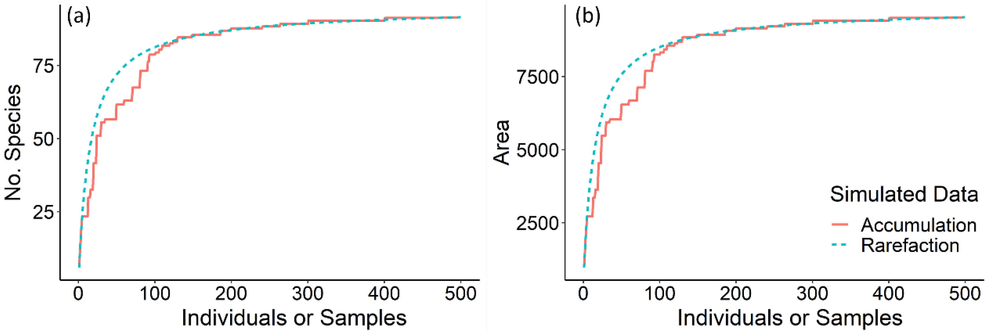
Species accumulation curves and rarefaction methods are well-developed approaches to standardize and control for sample size effects on biodiversity measures across datasets [23]. In essence, species accumulation curves record the total number species found as additional individuals (or samples) are collected. Such curves generally show the gradual accumulation of new species, but with an eventual levelling off (or asymptote) when additional collection yields no new species (Figure 1). Rarefaction methods re-sample random subsets of a cumulative species dataset to quantify the statistical expectations of species numbers that will be observed with increasing sample effort (Figure 1).
Here, we aim to understand the effect of sample size on the spatial extent of human activities documented within a specified area using participatory mapping. We hypothesize that spatial representation of a human activity (e.g., logging, hunting, fishing) is influenced by the number of participants akin to the way sampling effort influences biodiversity measures. To demonstrate this approach, we used a case study of small-scale fisheries targeting coral reefs in the central Philippines. We adapt the rarefaction curve concept to estimate the fisher sample size needed to map the maximum extent of fishing grounds within a specified area for a time series of participatory maps. To do so, we develop a way to estimate the sample size of fishers needed to map 90% of the extent of fishing grounds using a time series of participatory maps. By standardizing sampling, we aim to develop a method that (1) ensures that the spatial extent of an activity is documented accurately and (2) enables meaningful comparison among spatial datasets collected over different historical periods or at different locations. We build on concepts from biodiversity monitoring which pioneered methods for evaluating the influence of sample size on diversity measures.
2. Materials and Methods
2.1. Study Site
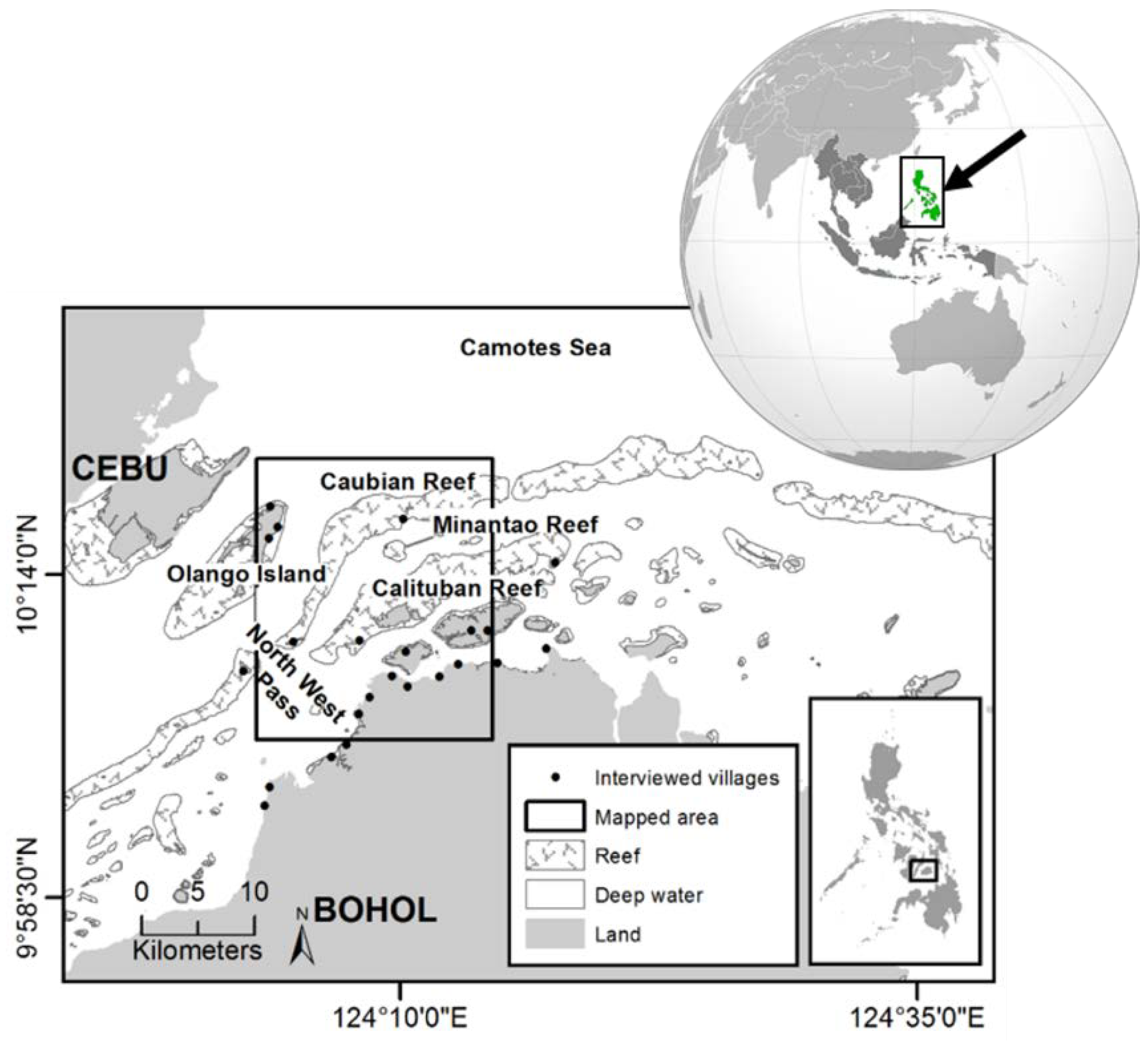
Our case study focused on mapping small-scale fisheries in the Danajon Bank ecosystem (Central Visayas, Philippines; 10°15′0’N, 124°8′0′E; Figure 2). Located in the Coral Triangle, the global center of marine biodiversity, the Danajon Bank supports many rural islands with limited infrastructure (e.g., many islands have no running water or electricity) and widespread poverty. Between 45% and 70% of the residents live below the Philippines poverty level. The region is adjacent to Cebu City, the second largest metropolitan area in the Philippines (2.8 million people). Communities in the region maintain a high reliance on marine resources and fishing is a primary livelihood. Fishers employ diverse fishing practices, enabling them to catch a diverse range of marine life [24]. Most fishers use outrigger canoe style boats. While there has been a rapid growth in the availability of engines, many fishers still use boats without engines (50% engine use in 2010) [5]. For this study, we focused on fishing that targeted a 19 × 22 km region in the central section of the Danajon Bank (hereafter, “study area” refers to the area demarcated by the bounding box in Figure 2).
2.2. Interviews and Participatory Mapping Procedures
To map spatial and temporal changes in fishing practices within the study area, we conducted semi-structured interviews with male fishers between July 2010 and April 2011 (of n = 391 respondents only 295 reported fishing in the study area). Hereafter, “sample size” refers to the 295 individuals who fished inside of the study area. Interviews took place in 23 randomly selected fishing communities. Because when we started the project we could not find a map that accurately identified the locations of all coastal villages, we created a map with key informants and collection of GPS points at villages. We randomly sampled 50% of the coastal villages within the study area as well as 50% of coastal villages within 10 km of the study area border. This larger sampling area ensured that we captured fishing effort by people who travelled to the study area to fish. While not previously verified for this region, at 10 km we found no individuals who fished within our study area [5].
When selecting villages, we stratified villages by geographic location (mainland, terrestrial island, caye), because it influenced the type of fishing methods practiced. Because Philippines census data are regularly collected by village health workers, they are highly knowledgeable about the livelihoods of community members. Thus, we randomly sampled 7% of full- and part-time male fishers within each village based on village-level census data and interviews with community health workers. Prior to random sampling, we also stratified fishers by age, focusing on fishers born before 1981, so we could capture people who had fished for a minimum of 15 years. We did not use snowball sampling because, in a pilot study, it greatly underestimated the diversity of fishing methods and fishing locations (Selgrath, unpublished data). Additionally, we did not use municipal lists of fishers because such lists greatly underestimated the number of fishers who were active in the region (Selgrath, unpublished data). We obtained written permission from mayors and oral permission from village leaders and respondents, as is customary in the Philippines. Methods were approved by The University of British Columbia’s Human Behavioural Research Ethics Board (H07- 00577).
For each interview, we first created an aspatial timeline of each individual’s life (e.g., marriage, birth of children) and fishing history (e.g., fishing methods, fishing effort). Next, we oriented fishers to the basemap, incorporating high spatial resolution SPOT-5 satellite images (10 × 10 m cells), where geographic features such as islands, reef geomorphology, and mangrove forests, were visible. The basemap also identified landmarks, such as municipal centers, ports, and marine protected areas (MPAs). The basemap (20 × 23 km) used during interviews was slightly larger than the study area (19 × 22 km) to allow subsequent cropping of map borders to remove edge effects. When we were confident respondents were oriented to the basemap, they directed us in drawing polygons around their current and past fishing grounds in the study area. This approach provided consistency in how polygons were drawn (e.g., minimum mapping units) and was useful because many fishers were uncomfortable drawing. Lastly, we made a spatially-referenced timeline of the attributes of each identified fishing ground. These attributes included: years fished; months per year fished; days per month fished; and fishing methods used at each fishing ground for every year from 1960 to 2010. We recorded increases or decreases in these attributes, as noted by the respondent. Here, we focus on annual fishing practices at ten-year intervals (e.g., 1960, 1970, 1980).
2.3. Integration of Maps Depicting Long-Term Fishing Effort
Our goal was to create maps of the annual maximum extent of all fishing in the study area at ten-year intervals (e.g., 1960, 1970). Upon completion of interviews, our first step was to prepare the hand drawn maps for further analysis by digitizing fishing polygons using heads-up digitizing in ArcGIS 10.1 (ESRI 2019). Then, for each respondent, their personal fishing ground polygons were linked to an attribute table with their reported fishing effort within said polygon (where fishing effort was measured as days per year fished). We repeated this map-joining process for 1960, 1970, 1980, 1990, 2000, and 2010, producing up to six maps for each respondent (Figure 3). After repeating this process for each respondent, we produced a total of 894 maps (295 respondents × 1–6 maps each) (Table 1). For consistency, all maps were converted to raster format (20 m cell size) and cropped to a consistent 19 × 22 km (418.0 km2) extent. Lastly, we created a set of maps depicting the maximum extent of the study area fished by all respondents in a given year (i.e., the maximum extent). To do so, we merged and dissolved all individuals’ fishing ground polygons for a given year. Further details of these calculations are available in Selgrath et al., 2017.
2.4. Rarefaction Curves
We used bootstrapping to evaluate whether the number of respondents influenced the maximum extent of fishing in the study area. Bootstrapping uses randomly selected subsets of data from a larger dataset, which are then compiled and analyzed over multiple (random) iterations. For our purposes, each iteration used a subset of respondents and their fishing ground polygons in a specified year [25]. Then for each iteration, we calculated the estimated extent of fishing. The size of respondent groups ranged from one to the maximum number of active fishers in that year (Table 1) and we executed ten iterations per respondent group. Thus, the iterations provided ten estimates of the extent of fishing for each sample size, but used different combinations of respondents. From these estimates, we calculated the mean estimated extent of fishing (along with confidence intervals) for each size of respondent group. This process was then repeated for six years: 1960, 1970, etc.
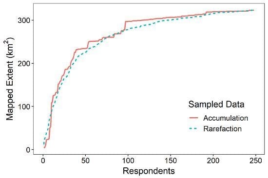
For each year, we graphed size of respondent group against two measures of fishing extent: the raw estimated area (to create area accumulation curves); and the mean estimated area based on bootstrapping (to create area rarefaction curves). These graphs allowed us to assess how the estimated extent of fishing varied over different respondent group sizes, as well as compare area accumulation curves and area rarefaction curves.
Next, we used the rarefaction curves to identify years with large enough sample sizes to see a “levelling off” of the estimated extent of fishing (i.e., reaching an asymptote). Using only the years that asymptoted, we determined the mean maximum fishing extent, as well as the mean sample size (across these same years) that captured 90% of the mean maximum extent. This mean sample size was then used as a minimum threshold for achieving an informative estimate of fishing extent, and importantly, allowed us to determine if samples from distant decades included a large enough number of respondents to be considered informative.
In years that did not reach an asymptote, we used modeling to predict the maximum spatial extent of fishing. To do so, we compared how the maximum spatial extent changed over time when estimated using three methods: raw field data (including years with few respondents); linear model predictions (excluding years with few respondents); and quadratic model predictions (excluding years with few respondents). In both models, the maximum extent of fishing was the dependent variable and the year was the independent variable. We compared the fit of the linear and quadratic models using r2 values and analysis of deviance. Analyses were conducted in R 3.6.1 (R core team, Vienna, Austria) and R code is available at https://github.com/jselgrath/AreaRarefactionCurves.
3. Results
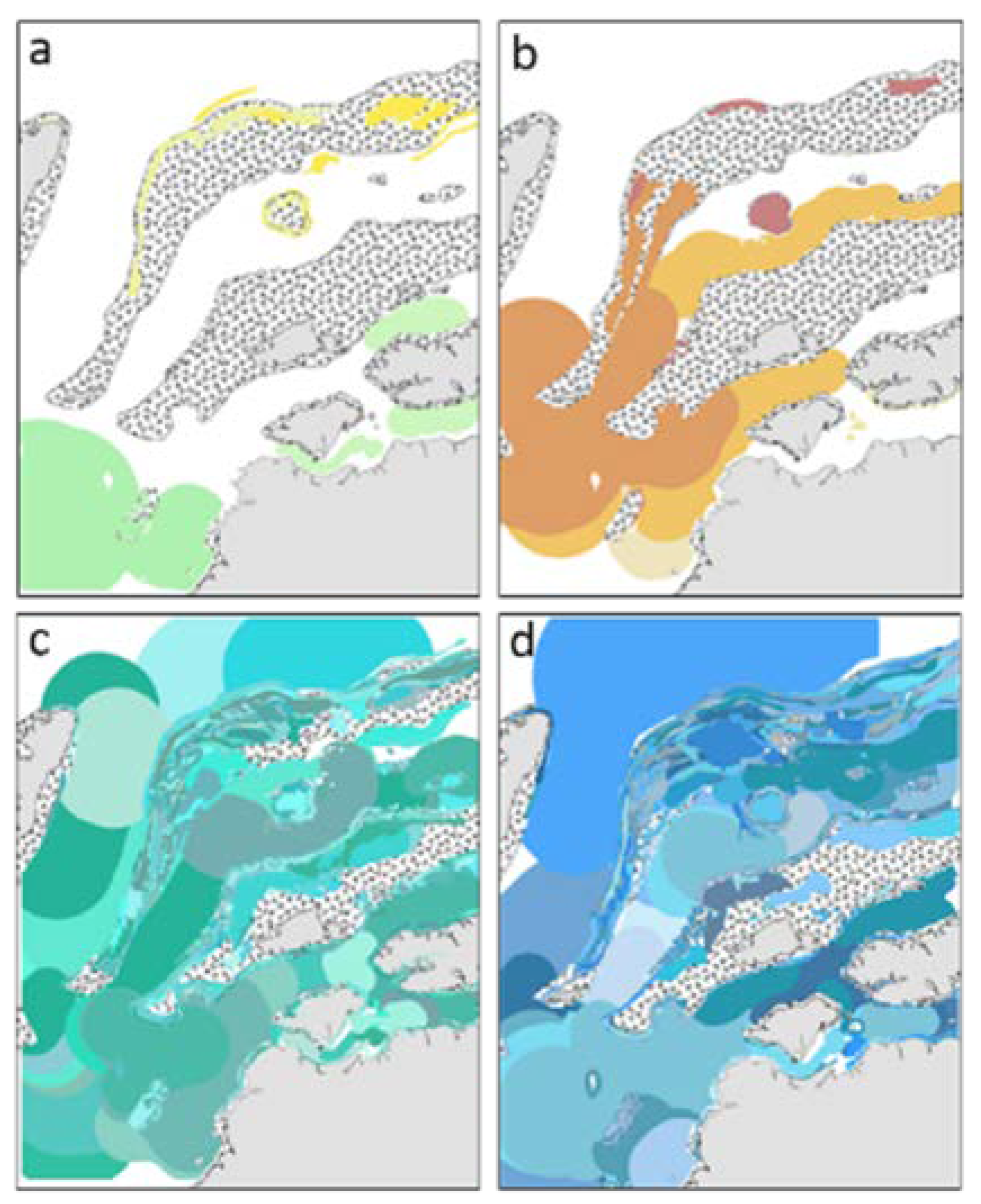
Our study interviewed 14 respondents who fished in 1960 and 248 respondents who fished in 2010. Reported fishing grounds were highly variable in extent and location (Figure 3). Maps of the estimated extent of fishing based on a small number of respondents were inconsistent and changed greatly based on individual respondents who happened to be included (Figure 4a,b). Maps synthesizing information from a larger number of respondents were more consistent (Figure 4c,d). Area accumulation curves and area rarefaction curves followed similar patterns to those observed in biodiversity sampling (Figure 1 and Figure 5). In particular, the estimated extent of fishing grounds increased as more respondents were included, but slowly leveled off (i.e., reached an asymptote) as greater numbers of respondents were added.
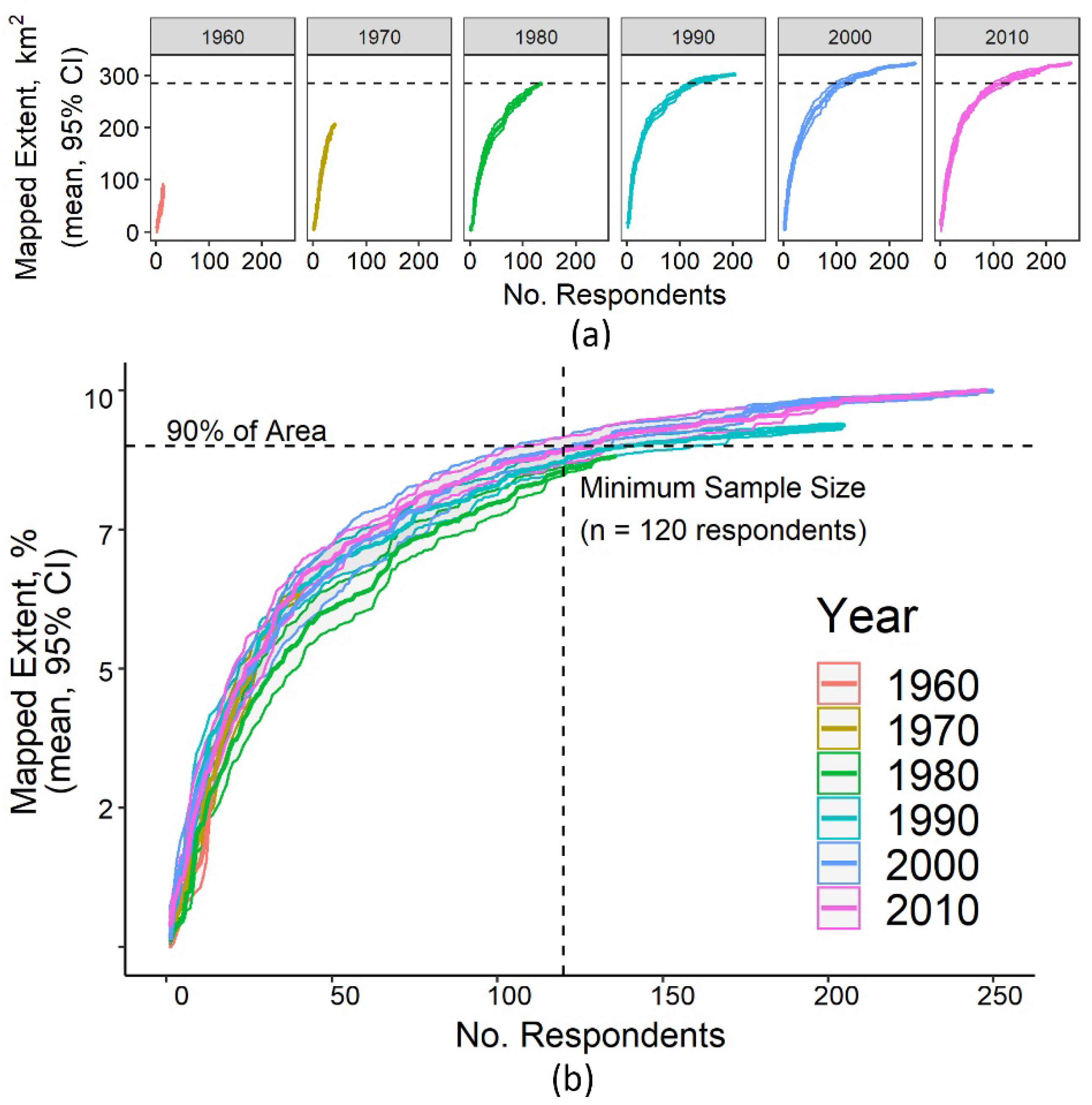
Our study included a mix of old and young respondents; thus, relatively few of our respondents were alive and fishing during the earliest years documented. Only three years (1990, 2000, 2010) had a large enough number of active fishers for the maximum extent fished to level off (reach an asymptote) with area rarefaction curves (Figure 6a). Using data from these three years, we found that the mean maximum extent of fishing was 319.94 km2 (89.4% of the ocean in the study area). The minimum sample size needed to map 90% of that area was 120 respondents (±3.7 se; range: 108–121). Using 120 respondents as a benchmark, we predict that our sample from 1980 also included a sufficient number of respondents (n = 136) to map 90% of the maximum extent of fishing in that year (Table 1; Figure 6). Two years had too few respondents to document 90% of the maximum extent of fishing accurately (1960: n = 14; 1970: n = 41; Figure 6).
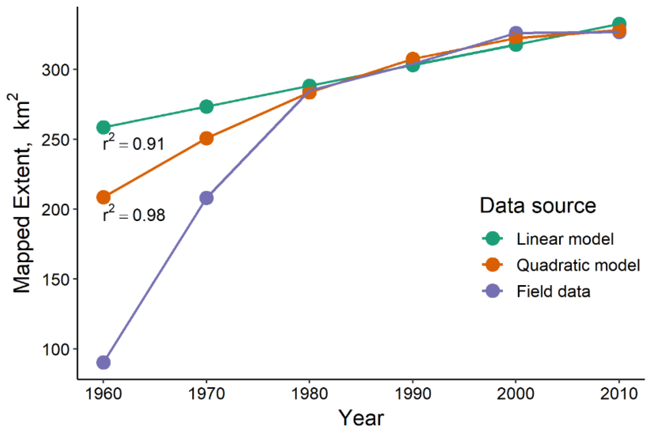
From 1960 to 2010, the raw field data showed a sharp increase in the maximum extent fished (a 254% increase in maximum extent). As these earliest three years did not level off (i.e. did not reach an asymptote); this indicates they did not have sufficient sample sizes to map the maximum extent of fishing. In contrast, when we predicted the maximum extent of fishing using modeling, there was a significant, but smaller increase over time (linear model = 11% increase; quadratic model = 36% increase). The two models were not significantly different in fit (X2 p = 0.09) (Figure 7), although the quadratic model had a higher r2 value (Linear r2 = 0.91; Quadratic r2 = 0.98).
4. Discussion
Our study demonstrated that sample size effects are important to consider when participatory maps are created to ensure that spatial patterns are accurately documented. We established three key benefits of using area rarefaction curves to improve the rigor of participatory mapping studies. First, we showed that area rarefaction curves can be used effectively to identify when participatory mapping projects have interviewed a sufficient number of people to accurately map the maximum extent of an activity. Here, we focused on the number of respondents needed to accurately capture the extent of human activities in a specified portion of a land- or seascape. Our results showed that when few respondents participated, participatory maps were inconsistent and incomplete, but became increasingly consistent and informative as the number of respondents grew. When a sufficient number of respondents was interviewed, the maximum extent mapped reached an asymptote. Beyond the sample size that reached an asymptote, additional respondents did not capture increasing extents of human impacts. Second, we established that standardizing for the number of survey respondents across different years allowed for more meaningful comparison, even when sample sizes differed, thus improving well-known limitations of local ecological knowledge (retrospective bias; individual and generational amnesia) [19,26,27]. In biodiversity monitoring, an established benefit of rarefaction curves is enabling meaningful comparison among locations. Therefore, we infer that a third benefit of area rarefaction curves will be to support comparisons among participatory maps from different places. Below, we explore the implications of these findings in other participatory mapping contexts.
4.1. How Much is Enough?
When the accuracy and detail of collected data are an important outcome from participatory mapping, a strong sampling design is essential. In the participatory mapping literature, however, the number of respondents included varies widely. A number of participatory mapping studies had small sample sizes and/or did not collect explicit demographic information about respondents. In some cases, the sample size of respondents was neither documented nor included in published literature (e.g., [28,29]). When sample sizes were published, participant numbers were frequently in the relatively small range of 10–50 respondents (e.g., [30,31,32,33]) or in the relatively large range of 100–400 respondents (e.g., [5,6,34,35]).
Our research demonstrates that one can quantify the minimum sample size needed to accurately map the extent of an activity, such as fishing. Using area rarefaction curves, we found that for our case study, a sample size of 120 individual respondents was needed to accurately map 90% of the spatial extent of fishing grounds in the Danajon Bank used by male fishers. It is estimated that 11,000 men currently fish full- and part-time in our study area [36]. Thus, the minimum sample size that we identified was 2.2% of the population of male fishers from the communities that we engaged in this study, or 1.1% of the total number of male fishers in the survey area. Since the Danajon Bank is crowded and supports an incredibly high diversity of fishing methods [24], we expect that the 1.1% minimum sample size was influenced by the significant amount of spatial overlap in the fishing grounds used by individuals and communities. Our mapping results suggest that a larger number of individuals may be needed to reach an asymptote in 1980 than in later years. Although the number of respondents in 1980 (n = 136) was larger than the minimum sample size (n = 120) that was suggested from 1990–2010 maps, the 1980 area rarefaction curves did not yet show signs of levelling off. Future research will need to address how to adjust minimum samples for participatory mapping in sparsely populated regions, or in situations where individual practices are over-dispersed and exhibit little spatial overlap.
4.2. Creating Robust Participatory Maps
Accurately mapping changes through time using retrospective interviews presents many challenges [18], including the fact that relatively few people have lived long enough to remember the distant past. Therefore, it may be necessary to randomly sample more people to include activities that are further back in time. It is easier to interview people who possess shorter memories, simply because there are more of them. Targeting elder individuals, using age-stratified sampling as we did here, is one strategy to improve estimates of the past [5,37]. However, when mapping the maximum extent of an activity, age-stratified sampling does not distinguish between change due to fluctuations in sample size, and change due to real differences between historic and present times. Area rarefaction curves, as demonstrated here, provide a powerful tool for ensuring that observed differences are not an artifact of sampling. In doing so, area rarefaction curves can support meaningful assessments of change over time, even for data-poor systems.
Our findings reiterate the importance of understanding how individuals who are interviewed for participatory mapping represent the total population. The individuals who participate in participatory mapping research can have a strong influence on participatory results, and a biased sample can completely change outcomes [38]. This point is poignant because the participatory mapping literature abounds with research that did not collect and/or provide information about how the number or demographic of respondents represents the community or population of interest (e.g., fishers, pastoralists, recreationalists). Here, fishers were identified through a combination of census data and interviews with village health workers, and respondents were chosen through random sampling. However, our results demonstrate that we could have saved resources (e.g., time and money) by interviewing a smaller number of individuals while still collecting accurate information. Alternatively, with a smaller sample size, we could have included a broader swath of fishers in our project. For example, we did not document the primarily inshore fishing by women and children [39]. Including a new group with widely differing spatial patterns would lead to a larger population that was being sampled and would, therefore, require a larger sample size, proportional to the new group sampled.
Since the field of participatory mapping developed with a focus on application, practitioners have placed less emphasis on engaging statistical design or on developing a theoretical framing to guide sampling [21]. For example, relatively few participatory mapping studies have incorporated randomized experimental design (but see, for example, [5,6,40]). Representational sampling of populations is challenging. Where demographic data do not exist, such information can be time consuming to collect, particularly in remote areas [41]. Where demographic data do exist, it can still be difficult to access. For example, we spent a full month visiting villages to collect existing census data and to identify fishers. Even in study sites with relatively small populations, thorough sampling can be difficult [42]. However, demographic information of participants is foundational for comparing spatial patterns over time and in different locations, as well as for ensuring that participatory maps accurately reflect the extent of an activity.
Choice of basemaps was an important and non-trivial component of the research. Participatory mapping uses a variety of basemaps, from sketch maps (participatory maps drawn freely, without a basemap), to published topographic and bathymetric maps, to satellite imagery. While sketch maps can be beneficial in some cases [41], they are not conducive to translating into GIS or for understanding collective patterns. This limitation arises because sketch maps are not drawn to a set scale or aligned with a standard geographic projection. Thus, sketch maps from different respondents are often unaligned and difficult to migrate to a digital platform [43]. Topographic and bathymetric maps, while highly standardized and beneficial for individuals familiar with such formats [30], may contain extraneous details that confuse participants or may miss important local landmarks [41]. As satellite imagery becomes universally accessible, there is great promise in using satellite imagery as basemaps. Through testing various approaches, we found that original satellite images were less effective than some sort of modified satellite images with additions, such as masking deep water, which focused respondents on geographic features that were visible in shallow water areas. Participants in our study were better able to orient themselves to maps that clearly identified locations such as ports, rivers, and village centers.
4.3. Essential Role of Maps
Participatory mapping has emerged from an intersection of disciplines in support of diverse goals that range from building social capital to expanding spatial information [21]. For projects whose purposive goals are focused on building capacity, fostering trust, and enhancing social identity, creating highly accurate or complete maps may be a lower priority for the mapping process. In such cases, mapping conducted during community workshops may not need to account for the number of respondents or how representative they are of the community as a whole. Participatory mapping endeavors may focus on sharing information between different generations within a community, establishing traditional land for indigenous communities, or on engaging with leaders in the community [44,45,46]. However, when quantitative spatial estimates are an important project outcome, a strong sampling design is essential and can be improved by the rarefaction approaches presented here.
Conservation exemplifies a critically important field which benefits from the long-term, spatial perspective accessible through participatory mapping. To sharpen the effectiveness of conservation, it is valuable to establish a more comprehensive understanding of how human activities develop, and in turn influence the distribution of species and habitats. However, many social–ecological systems are data-poor and lack historical data of any kind. In situations where no long-term data exist, participatory mapping (and local ecological knowledge, more broadly) provide an invaluable method for filling this gap [47]. In many cases, spatial data—obtained through participatory mapping—is essential for accurately tracking change, because non-spatial data may severely underestimate impacts. In Danajon Bank fisheries, for example, non-spatial data (total effort by all fishers) estimated a 250% increase in fishing effort (1960–2010) [5,24]. However, spatially explicit fishing effort (mean fishing effort in all grid cells)—documented through participatory mapping—identified that fishing effort increased 1800% (1960–2010). This 8.6-fold difference in these two estimates occurred because aggregating data over large areas can obscure important local trends [48].
5. Conclusions
Participatory maps are widely used to depict how human activities (e.g., fishing, logging, pastoral systems) vary over space and time, yet the accuracy of such maps is rarely accounted for. In conservation, maps of human activities can serve as a foundation for understanding how humans affect the environment around them. Such maps can delineate the location, frequency, and intensity of human practices during a single time period or longitudinally. When participatory maps of human practices are paired with maps of natural systems, their union can be used to delineate sustainable activities from those that are damaging. In the Danajon Bank, participatory mapping revealed that fishing effort increased more than 1800%, and that this increase was due to the growing number of individuals fishing, rather than to changes in individual fishing effort [5,24]. In contrast, non-spatial measures greatly underestimated the severity of this change. However, the power of participatory mapping to document long-term change ultimately depends on the accuracy of the maps themselves. Area rarefaction curves provide a straightforward approach to make an informed decision about how many individuals to interview, and how to address changes in the number of respondents who were active during different times. Consequently, area rarefaction curves can ensure that observed differences are not an artifact of sampling. By allowing participatory mapping to standardize for the effects of sample size, area rarefaction curve can support meaningful assessments of change over time, even for data-poor systems.
Author Contributions
Conceptualization, J.C.S. and S.E.G.; methodology, J.C.S.; software J.C.S. and S.E.G.; formal analysis, J.C.S.; data curation, J.C.S.; writing—original draft preparation, J.C.S.; writing—review and editing, J.C.S. and S.E.G.; visualization, J.C.S.; funding acquisition, J.C.S. and S.E.G.
Funding
This research was funded by Planet Action, The Explorer’s Club, Point Defiance Zoo and Aquarium. JCS was funded by a Rick Hansen Man in Motion Scholarship and a Fulbright Scholarship. SEG was supported by NSERC-DG.
Acknowledgments
We thank the communities of the Danajon Bank, Project Seahorse Foundation for Marine Conservation (now ZSL Philippines), SeaLifeBase, the John G. Shedd Aquarium, and the International Rice Research Institute for their support. We also thank G. Sucano, B. Calinijan, V. Calinawan, V. Lazo, S. Ravensbergen, I. Eddy, and J. Cristiani for help in the field and lab. S. Foster, S. Tomschea, D. Kleiber, L. Aylesworth, T. Loh, and C. Walters provided insights. A.C.J. Vincent was instrumental in developing the project.
Conflicts of Interest
The authors declare no conflict of interest. The funders had no role in the design of the study; in the collection, analyses, or interpretation of data; in the writing of the manuscript, or in the decision to publish the results.
References
- Kroodsma, D.A.; Mayorga, J.; Hochberg, T.; Miller, N.A.; Boerder, K.; Ferretti, F.; Wilson, A.; Bergman, B.; White, T.D.; Block, B.A.; et al. Tracking the global footprint of fisheries. Science 2018, 908, 904–908. [Google Scholar] [CrossRef] [PubMed]
- Richards, D.R.; Tunçer, B.; Tunçer, B. Using image recognition to automate assessment of cultural ecosystem services from social media photographs. Ecosyst. Serv. 2018, 31, 318–325. [Google Scholar] [CrossRef]
- Berkes, F. Sacred Ecology, 3rd ed.; Routledge: New York, NY, USA, 2012; ISBN 978-0415517324. [Google Scholar]
- McMillen, H.L.; Ticktin, T.; Friedlander, A.M.; Jupiter, S.D.; Thaman, R.; Campbell, J.; Veitayaki, J.; Giambelluca, T.; Nihmei, S.; Rupeni, E.; et al. Small islands, valuable insights: Systems of customary resource use and resilience to climate change in the Pacific. Ecol. Soc. 2014, 19, 44. [Google Scholar] [CrossRef]
- Selgrath, J.C.; Gergel, S.E.; Vincent, A.C.J. Incorporating spatial dynamics greatly increases estimates of long-term fishing effort: A participatory mapping approach. ICES J. Mar. Sci. 2017, 75, 210–220. [Google Scholar] [CrossRef]
- Aylesworth, L.; Phoonsawat, R.; Suvanachai, P.; Vincent, A.C.J. Generating spatial data for marine conservation and management. Biodivers. Conserv. 2016, 26, 383–399. [Google Scholar] [CrossRef]
- Gergel, S.E. New Directions in Landscape Pattern Analysis and Linkages with Remote Sensing. In Understanding Forest Disturbance and Spatial Pattern: Remote Sensing and GIS Approaches; Wulder, M., Franklin, S.E., Eds.; Taylor and Francis Group: Boca Raton, FL, USA, 2007; pp. 173–208. [Google Scholar]
- Gergel, S.E.; Stange, Y.; Coops, N.C.; Johansen, K.; Kirby, K.R. What is the value of a good map? An example using high spatial resolution imagery to aid riparian restoration. Ecosystems 2007, 10, 688–702. [Google Scholar] [CrossRef]
- Tulloch, V.J.; Possingham, H.P.; Jupiter, S.D.; Roelfsema, C.M.; Tulloch, A.I.T.; Klein, C.J. Incorporating uncertainty associated with habitat data in marine reserve design. Biol. Conserv. 2013, 162, 41–51. [Google Scholar] [CrossRef] [Green Version]
- Wulder, M.A.; Hall, R.J.; Coops, N.C.; Franklin, S.E. High spatial resolution remotely sensed data for ecosystem characterization. Bioscience 2004, 54, 511. [Google Scholar] [CrossRef]
- Roelfsema, C.M.; Phinn, S.R. Validation. In Coral Reef Remote Sensing: A Guide for Multi-Level Sensing Mapping and Assessment; Goodman, J.A., Purkis, S.J., Phinn, S.R., Eds.; Springer: Dordrecht, The Netherlands, 2013; pp. 375–401. [Google Scholar]
- Thompson, S.D.; Gergel, S.E. Conservation implications of mapping rare ecosystems using high spatial resolution imagery: Recommendations for heterogeneous and fragmented landscapes. Landsc. Ecol. 2008, 23, 1023–1037. [Google Scholar] [CrossRef]
- Teixeira, J.B.; Martins, A.S.; Pinheiro, H.T.; Secchin, N.A.; Leão de Moura, R.; Bastos, A.C. Traditional Ecological Knowledge and the mapping of benthic marine habitats. J. Environ. Manag. 2013, 115, 241–250. [Google Scholar] [CrossRef]
- Chambers, R. Participatory Rural Appraisal (PRA): Analysis of Experience. World Dev. 1994, 22, 1253–1268. [Google Scholar] [CrossRef]
- Selgrath, J.C.; Roelfsema, C.M.; Gergel, S.E.; Vincent, A.C.J. Mapping for Coral Reef Conservation: Comparing the Value of Participatory and Remote Sensing Approaches. Ecosphere 2016, 7, e01325. [Google Scholar] [CrossRef]
- Foale, S.J. Assessment and management of the trochus fishery at West Nggela, Solomon Islands: An interdisciplinary approach. Ocean Coast. Manag. 1998, 40, 187–205. [Google Scholar] [CrossRef]
- Lauer, M.; Aswani, S. Integrating indigenous ecological knowledge and multi-spectral image classification for marine habitat mapping in Oceania. Ocean Coast. Manag. 2008, 51, 495–504. [Google Scholar] [CrossRef]
- Neis, B.; Schneider, D.C.; Felt, L.; Haedrich, R.L.; Fischer, J.; Hutchings, J.A. Fisheries assessment: What can be learned from interviewing resource users? Can. J. Fish. Aquat. Sci. 1999, 56, 1949–1963. [Google Scholar] [CrossRef]
- O’Donnell, K.P.; Molloy, P.P.; Vincent, A.C.J. Comparing Fisher Interviews, Logbooks, and Catch Landings Estimates of Extraction Rates in a Small-Scale Fishery. Coast. Manag. 2012, 40, 594–611. [Google Scholar] [CrossRef]
- Gavin, M.C.; Solomon, J.N.; Blank, S.G. Measuring and monitoring illegal use of natural resources. Conserv. Biol. 2010, 24, 89–100. [Google Scholar] [CrossRef]
- Brown, G.; Kyttä, M. Key issues and research priorities for public participation GIS (PPGIS): A synthesis based on empirical research. Appl. Geogr. 2014, 46, 122–136. [Google Scholar] [CrossRef]
- MacArthur, R.H.; Wilson, E.O. The Theory of Island Biogeography; Princeton University Press: Princeton, NJ, USA, 1967. [Google Scholar]
- Gotelli, N.J.; Colwell, R.K. Quantifying biodiversity: Procedures and pitfalls in the measurement and comparison of species richness. Ecol. Lett. 2001, 4, 379–391. [Google Scholar] [CrossRef]
- Selgrath, J.C.; Gergel, S.E.; Vincent, A.C.J. Shifting Gears: Diversification, intensification and effort increases of small-scale fisheries. PLoS ONE 2018, 13, e0190232. [Google Scholar] [CrossRef]
- Payton, M.E.; Greenstone, M.H.; Schenker, N. Overlapping confidence intervals or standard error intervals: What do they mean in terms of statistical significance? J. Insect Sci. 2003, 3, 34. [Google Scholar] [CrossRef] [PubMed]
- Papworth, S.; Rist, J.; Coad, L.; Milner-Gulland, E.J. Evidence for shifting baseline syndrome in conservation. Conserv. Lett. 2009, 2, 93–100. [Google Scholar] [CrossRef]
- Daw, T.M. Shifting baselines and memory illusions: What should we worry about when inferring trends from resource user interviews? Anim. Conserv. 2010, 13, 534–535. [Google Scholar] [CrossRef]
- Gonzalez, R.M. Joint learning with GIS: Multi-actor resource management. Agric. Syst. 2002, 73, 99–111. [Google Scholar] [CrossRef]
- Cronkleton, P.; Albornoz, M.A.; Barnes, G.; Evans, K. Social Geomatics: Participatory Forest Mapping to Mediate Resource Conflict in the Bolivian Amazon. Hum. Ecol. 2010, 38, 65–76. [Google Scholar] [CrossRef]
- Klain, S.C.; Chan, K.M.A. Navigating coastal values: Participatory mapping of ecosystem services for spatial planning. Ecol. Econ. 2012, 82, 104–113. [Google Scholar] [CrossRef]
- Lestrelin, G.; Bourgoin, J.; Bouahom, B.; Castella, J.C. Measuring participation: Case studies on village land use planning in northern Lao PDR. Appl. Geogr. 2011, 31, 950–958. [Google Scholar] [CrossRef]
- Halme, K.J.; Bodmer, R.E. Correspondence between Scientific and Traditional Ecological Knowledge: Rain Forest Classification by the Non-Indigenous Ribereños in Peruvian Amazonia. Biodivers. Conserv. 2006, 16, 1785–1801. [Google Scholar] [CrossRef]
- Eddy, I.M.S.; Gergel, S.E.; Coops, N.C.; Henebry, G.M.; Levine, J.; Zerriffi, H.; Shibkov, E. Integrating remote sensing and local ecological knowledge to monitor rangeland dynamics. Ecol. Indic. 2017, 82, 106–116. [Google Scholar] [CrossRef]
- Fagerholm, N.; Käyhkö, N.; Ndumbaro, F.; Khamis, M. Community stakeholders’ knowledge in landscape assessments—Mapping indicators for landscape services. Ecol. Indic. 2012, 18, 421–433. [Google Scholar] [CrossRef]
- Moreno-Báez, M.; Orr, B.J.; Cudney-Bueno, R.; Shaw, W.W. Using Fishers’ Local Knowledge to Aid Management At Regional Scales: Spatial Distribution Of Small-Scale Fisheries in the Northern Gulf of California, Mexico. Bull. Mar. Sci. 2010, 86, 339–353. [Google Scholar]
- Selgrath, J.C. Spatial and Temporal Changes in Small-Scale Fisheries on Coral Reefs, and Their Impact on Habitats; The University of British Columbia: Vancouver, BC, Canada, 2017. [Google Scholar]
- Herrmann, S.M.; Sall, I.; Sy, O. People and pixels in the Sahel: A study linking coarse-resolution remote sensing observations to land users’ perceptions of their changing environment in Senegal. Ecol. Soc. 2014, 19, 29. [Google Scholar] [CrossRef]
- Brown, G.; Kelly, M.; Whitall, D. Which “public”? Sampling effects in public participation GIS (PPGIS) and volunteered geographic information (VGI) systems for public lands management. J. Environ. Plan. Manag. 2013, 57, 190–214. [Google Scholar]
- Kleiber, D.; Harris, L.M.; Vincent, A.C.J. Improving fisheries estimates by including women’s catch in the Central Philippines. Can. J. Fish. Aquat. Sci. 2014, 71, 656–664. [Google Scholar] [CrossRef]
- Leopold, M.; Guillemot, N.; Rocklin, D.; Chen, C. A framework for mapping small-scale costal fisheries using fishers’ knowledge. ICES J. Mar. Sci. 2014, 71, 1781–1792. [Google Scholar] [CrossRef]
- Smith, D.A. Participatory mapping of communty lands and hunting yields among the Bugle of Western Panama. Hum. Organ. 2003, 62, 332–343. [Google Scholar] [CrossRef]
- Altmann, B.A.; Jordan, G.; Schlecht, E. Participatory mapping as an approach to identify grazing pressure in the Altay Mountains, Mongolia. Sustainability 2018, 10, 1960. [Google Scholar] [CrossRef]
- Bauer, K. On the politics and the possibilities of participatory mapping and GIS: Using spatial technologies to study common property and land use change among pastoralists in Central Tibet. Cult. Geogr. 2009, 16, 229–252. [Google Scholar] [CrossRef]
- Peluso, N.L. Whose Woods Are These? Counter-Mapping Forest Territories in Kalimantan, Indonesia. Antipode 1995, 27, 383–406. [Google Scholar] [CrossRef]
- Herlihy, P.H.; Knapp, G. Maps of, by, and for the Peoples of Latin America. Hum. Organ. 2003, 62, 303–314. [Google Scholar] [CrossRef]
- Chambers, R. Participatory Mapping and Geographic Information Systems: Whose Map? Who is Empowered and Who Disempowered? Who Gains and Who Loses? Electron. J. Inf. Syst. Dev. Ctries. 2006, 25, 1–11. [Google Scholar] [CrossRef] [Green Version]
- Thornton, T.F.; Scheer, A.M. Collaborative engagement of local and traditional knowledge and science in marine environments: A review. Ecol. Soc. 2012, 17, 8. [Google Scholar] [CrossRef]
- Walters, C.J. Folly and fantasy in the analysis of spatial catch rate data. Can. J. Fish. Aquat. Sci. 2003, 60, 1433–1436. [Google Scholar] [CrossRef]
Figure 1.
Examples of simulated graphs showing contrasting patterns between accumulation and rarefaction methods when using different sample sizes for (a) number of species observed and (b) estimated extent of fishing. Both simulated datasets exhibit an asymptotic (leveling off) behavior. Beyond that point collecting additional samples (species or maps) does not lead to new information on the total number of species or maximum extent of human activities.

Figure 2.
Danajon Bank coral reef in the Central Visayas, Philippines, where fishers were interviewed to create long-term maps of fishing grounds, as shown in Figure 3. The study area, within which respondents mapped their fishing grounds, is outlined by the black box. The 418.0 km2 (19 × 22 km) study area contained 354.1 km2 of ocean.

Figure 3.
Example maps of reported fishing grounds used in 2010 by six individual fishers (a–f), collected through participatory mapping. Maps of individuals’ fishing grounds, such as the examples shown here, were combined to make maps of the maximum extent of fishing in a year at decadal intervals.

Figure 4.
Estimated extent of fishing using small (panels a,b) and large (panels c,d) numbers of respondents. Maps depict overlap of fishing grounds from random subsets of fishers with small (n = 5) and large (n = 125) numbers of respondents.
Figure 4.
Estimated extent of fishing using small (panels a,b) and large (panels c,d) numbers of respondents. Maps depict overlap of fishing grounds from random subsets of fishers with small (n = 5) and large (n = 125) numbers of respondents.

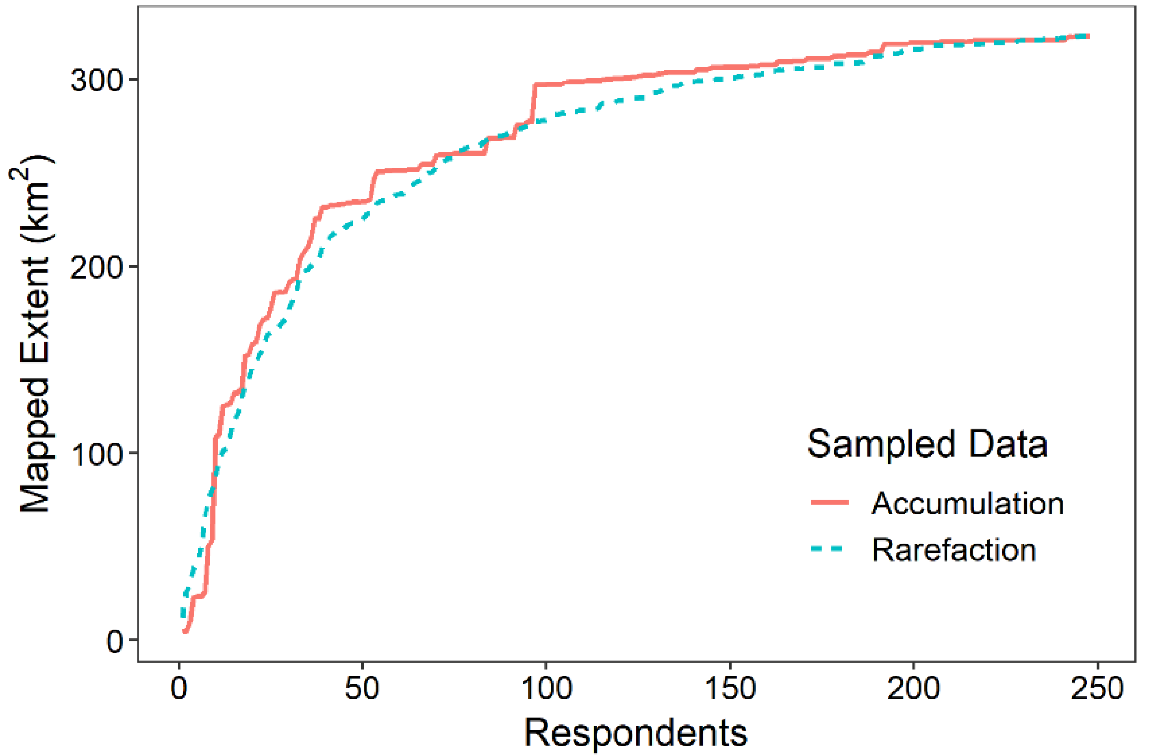
Figure 5.
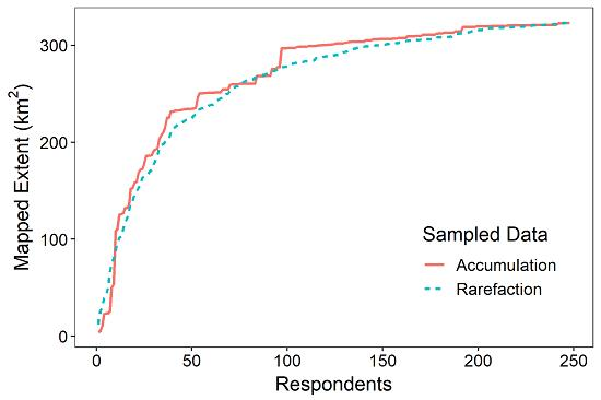
Two methods showed changes in the estimated extent of fishing grounds (in 2010) when different sample sizes of fishers were surveyed. The approach using an area accumulation curve represents one sequence for adding additional survey respondents. The approach using the area rarefaction curve was implemented through repeat resampling of respondents to create ten possible combinations of fishing grounds (ten for each number of respondents), and then plotting the mean estimated extent.
Figure 5.
Two methods showed changes in the estimated extent of fishing grounds (in 2010) when different sample sizes of fishers were surveyed. The approach using an area accumulation curve represents one sequence for adding additional survey respondents. The approach using the area rarefaction curve was implemented through repeat resampling of respondents to create ten possible combinations of fishing grounds (ten for each number of respondents), and then plotting the mean estimated extent.

Figure 6.
Historical resource use captured by participatory mapping and accounting for increasing numbers of maps over time. Panel (a) shows respondent numbers necessary to capture 90% of the maximum extent of fishing (estimated as per panel (b)). The percentage of the maximum extent captured in mapping varied across decades in part because information was gathered from fewer respondents (e.g., in more distant years, some respondents were not yet born). Vertical dashed line identifies the minimum number of respondents (n = 120) needed to capture 90% of the mean maximum fished area. Panel (b) shows separate rarefaction curves as per panel (a) for each of six decades (1960–2010), depicting the estimated extent of fishing grounds as a percentage of the mean cumulative area of fishing grounds. Notably, only three recent decades reached an asymptote (1990, 2000, 2010), signaling that sufficient sampling was achieved in those decades. The mean maximum extent of fishing grounds (estimated from these three decades) was 319.94 km2.

Figure 7.
Three methods for quantifying how the maximum extent of fishing changed over time (1960–2010). The field data estimated a sharp increase in the spatial extent of fishing over time. In contrast, linear and quadratic models (built excluding years with small numbers of actively fishing respondents) showed a relatively smaller increase in the maximum extent of fishing grounds. There was no significant difference between the fit of linear and quadratic models.


Table 1.
Information about the maximum extent of fishing, the total number of respondents interviewed, and the mean number of respondents needed to reach the 90% area target in that year. Statistics only include information from samples that met the 90% area threshold; thus statistics from two earlier years (1960, 1970) are not included due to insufficient sample sizes.
| Year | Extent Mapped (max, km2) | Extent Mapped (90%, km2) | No. Respondents (total) | No. Respondents (mean (se)) |
|---|---|---|---|---|
| 1960 | 91.14 | 82.02 | 14 | NA |
| 1970 | 209.12 | 188.21 | 41 | NA |
| 1980 | 284.99 | 256.49 | 136 | 134.5 (0.4) |
| 1990 | 303.47 | 273.13 | 205 | 120.7 (6.2) |
| 2000 | 322.90 | 290.61 | 250 | 107.7 (8.5) |
| 2010 | 323.10 | 290.79 | 248 | 115.5 (9.2) |
© 2019 by the authors. Licensee MDPI, Basel, Switzerland. This article is an open access article distributed under the terms and conditions of the Creative Commons Attribution (CC BY) license (http://creativecommons.org/licenses/by/4.0/).
Share and Cite
MDPI and ACS Style
Selgrath, J.C.; Gergel, S.E. How Much is Enough? Improving Participatory Mapping Using Area Rarefaction Curves. Land 2019, 8, 166. https://0-doi-org.brum.beds.ac.uk/10.3390/land8110166
AMA Style
Selgrath JC, Gergel SE. How Much is Enough? Improving Participatory Mapping Using Area Rarefaction Curves. Land. 2019; 8(11):166. https://0-doi-org.brum.beds.ac.uk/10.3390/land8110166
Chicago/Turabian StyleSelgrath, Jennifer C., and Sarah E. Gergel. 2019. "How Much is Enough? Improving Participatory Mapping Using Area Rarefaction Curves" Land 8, no. 11: 166. https://0-doi-org.brum.beds.ac.uk/10.3390/land8110166
Note that from the first issue of 2016, this journal uses article numbers instead of page numbers. See further details here.