Chaos in Motion: Measuring Visual Pollution with Tangential View Landscape Metrics


Department of Grassland and Landscape Studies, University of Life Sciences in Lublin, Akademicka 15 St., 20-950 Lublin, Poland
Land 2020, 9(12), 515; https://0-doi-org.brum.beds.ac.uk/10.3390/land9120515
Submission received: 21 November 2020
/
Revised: 8 December 2020
/
Accepted: 10 December 2020
/
Published: 12 December 2020
(This article belongs to the Special Issue Conditions, Effects and Costs of Spatial Chaos)
Abstract
:Visual pollution (VP) in the form of outdoor advertisements (OA) is a threat to landscape physiognomy. Despite their proven usefulness in landscape aesthetic studies, landscape metrics have not yet been applied to address the phenomenon of VP. To fill this knowledge gap, a methodological framework for the measurement of VP using tangential view landscape metrics is proposed, which is accompanied by statistically significant proofs. Raster products derived from aerial laser scanning data were used to characterize two study areas with different topographic conditions in the city of Lublin, East Poland. The visibility of the cityscape in motion was simulated through viewshed measurements taken at equal intervals in the forwards and backwards directions along pedestrian walkways. The scrutinized tangential view landscape metrics (visible area, maximum visible distance, skyline, Shannon depth, view depth line) was the object of a two-fold interpretation wherein the spatial occurrence of VP as well as its impacts on the visual landscape character (VLC) were examined. The visible area metrics were found to be highly sensitive VP indicators. The maximum visible distance metrics provided evidence for the destructive effect of OA on view corridors. The Shannon depth and depth line metrics were not found to be statistically significant indicators of VP. Results from directional viewshed modelling indicate that distortion in the analyzed cityscape physiognomy depends on the view direction. The findings allow for particular recommendations with practical implementations in land use planning, which are discussed along with limitations to our proposed methods.
1. Introduction
1.1. Visual Pollution as Spatial Chaos
Maslow’s hierarchy of needs [1] as graphically formalized by Charles McDermid [2], organizes human needs from the basic to the higher-order, placing the aesthetic needs, such as appreciation and search for beauty [3], at the very top. According to this hierarchy, physiological needs (sustenance) precede social needs (friendship), which in turn precede cognitive needs (education). With regard to landscapes, OA generate income, which allows beneficiaries to meet basic needs. Furthermore, citizens may locate basic needs such as food or shelter through exposure to OA. Under certain conditions, people may seek higher-order needs prior to basic ones. However, basic needs typically supersede higher-order needs. This is the case for the post-socialist urban landscape [4,5], to which this research concerns.
Due to the precedence of economic development, OA proliferate in cityscapes without consideration of the aesthetic issues associated with exposure to such complex additions to the landscape [6]. As such, without aesthetic consideration, the addition of OA to a landscape may be considered a form of spatial chaos—a phenomenon of visual landscape devastation [7]. Superficially, the manifestation of this kind of spatial chaos in urban landscapes may then be explained as a consequence of neglecting higher-order needs with regard to landscape aesthetics. However, such problems pertaining to the aesthetics of landscapes and specifically, to the physiognomy of cityscapes, require a scientific explanation on the basics of visual landscape theory [8,9] as well as landscape aesthetic indicator systems development [10]. Towards this end, the research contained herein has focused on VP [11] as a form of spatial chaos.
In the scientific literature, cities [12] rather than semi-natural landscapes or protected areas [5,13] are the most common setting in which VP has been described. São Paulo, Brazil has become an iconic city with respect to VP, where the Clean City Law was passed in order to diminish the effects of VP [14]. In addition to the aesthetic values of the cityscape, work in metro Manila, Philippines has focused on culturally alienating patterns that have been dispersed through advertised products [15]. Conversely, outdoor advertisement campaigns have been used to encourage and develop a multicultural national identity in Malaysia [16]. Cities in Iran struggle with the aesthetic and functional chaos imposed by building facades [17,18] and transit ways [19]. The propagation of OA that arose as a result of post-socialist economic rushes [5,20,21,22,23,24] is a prime example of spatial chaos in the form of VP that is the result of a lack of legal regulations pertaining to landscape physiognomy. In Polish law, the issue of VP was formalized in 2015. Following the example of Scenic America (a non-profit organization against VP), in Poland, the long-awaited landscape aesthetic improvement arrived mainly in thanks to the bottom-up initiatives of NGO’s (e.g., Miastomojeawnim/miastomoje.org).
VP is a relatively new concept in the international literature and as such, is the subject of active discussion. Generally, VP is defined as the compounded effect of disorder, and excess of various objects and graphics in a landscape [25,26]. Some research refers more specifically to street garbage, GSM towers [27], and brightly colored plastic bags [28] as types of VP. Some research includes light pollution as a type of VP phenomenon [29], while others do not [30]. Elena Enache (2012) defines VP as damage to the landscape issue, in a manner which can be perceptible to the human visual sense, and with effects on the psyche of the person [31]. The scientific literature proves there to be a number of adverse mental and physical effects of exposure to VP. VP has been found to contribute to a loss of cultural identify [15]. More generally, the content of OA can induce negative emotions, which cause stress [32]. Adverse physical effects of exposure to VP include eye fatigue and distraction in drivers, which decrease road safety [33].
The most consistently recognized symptom of VP is an excess of OA with contrasting colors and content, which create an oversaturation of anthropogenic visual information within a landscape. For the purposes of this research, VP is defined as the occlusion of the human field of view by OA features, which is strong enough to disturb the perceived character of a landscape. This definition refers to the impact of OA on the observer’s field of view in terms of visual landscape occlusion and distortion. As such, this study on VP is situated in the context of contemporary landscape aesthetic research [34] as well as VLC theory [35]. Despite the lack of consensus on the definition of VP, its sources and effects are quite well described in the scientific literature. However, there are still no guidelines that speak to when OA become VP. Some attempts have been undertaken by Chmielewski [23], who indicated that a cityscape tends to be evaluated as visually polluted when more than seven OA impact the observer’s field of view. These findings refer to a particular case study and result from subjective opinions of pedestrians. Usually, a single OA is not considered VP unless exposure to it is in high contrast to the landscape background. Furthermore, places like NY Times Square attract tourists with light from OA. In such a case, advertising as an artistic work can also be visually attractive. This makes VP threshold estimation difficult as no unified approach or guidelines can be accepted globally. To address this challenge, this research framework uses a quantified approach that divides metric values into quartiles where the third quartile is regarded as the VP threshold (details in Section 2.5). Beyond the two case-study areas (Section 2.1), different proportions, as well as exceptions, can be adapted to meet the city officials’ guidelines in practice. However, these considerations are beyond the scope of this study.
With this context in mind, the VP measurement methods and results contained herein provide insight to local urban planning authorities as well as to landscape aesthetic researchers.
1.2. Visibility Metrics for Visual Pollution Assessment
Methodological approaches to VP (also reviewed by Wakil, [36]) include descriptive-analytic methods [37], cumulative area analysis [38], social identity semiotic analysis [16], multi-temporal street-level photo comparisons [4,39] socio-economic [40] or spatio-political profiles description [15,22] opinion surveys [6,12] as well as the design concepts of a street furniture and media facade [41]. Importantly, three semi-automated VP tools have been proposed: close range photogrammetry [42], citizen science mapping [24] as well as image recognition and deep learning techniques [27].
However, to the best of this author’s knowledge, VP has not been the object of analysis with the use of landscape metrics, especially those related to visibility analysis. Landscape metrics have been proven to be useful tools for mapping landscape aesthetic values [43], especially when coupled with viewshed analysis [44]. Moreover, contemporary solutions in the field of landscape metrics development, which integrate the Shannon entropy theory (details in Section 1.3) with the visibility analysis, open up new possibilities in the field of VP diagnosis.
In landscape studies, viewshed methods are applied to raster data to estimate the visible part of the landscape. As viewshed methods identify the visible pixels along a sightline, they are considered to be a two-dimensional (2D) analysis. However, 2.5D analysis is possible by considering visible landscape features as vertical columns that extend between a digital terrain model (DTM) and a digital surface model (DSM) [45]. Such 2.5D analyses are preferable to 2D analyses, which result in visible area overestimation when 2D viewsheds are used as field of view (FoV) surrogates [46]. Accordingly, 2.5D tangential view analyses have been successfully implemented in several studies [47,48,49,50,51,52] and were thus applied in this experiment (described in Section 2.5).
Furthermore, the phenomenon of visibility is most commonly considered as a static relationship between the observer (a vantage point) and a visible area [53]. In reality however, the perception of visual landscapes likely takes place in motion (as the observer moves between vantage points). Therefore, we accounted for this by applying a directional view sequence approach inspired by Sectoral Analysis of Landscape Interiors [54] (the directional view sequence details are described in the method section).
1.3. Measuring Spatial Chaos
Landscapes are spatio-temporal systems of hierarchically related abiotic, biotic, and anthropogenic elements [55]. However, high levels of complexity and unpredictability mean that chaos is also a part of landscape systems. A diversity of elements and processes, combined with knowledge of the existence of an organizational plan, determine the aesthetic attractiveness of a landscape system, which is a form of organized chaos [56].
To understand these complexities, landscape research methods break down landscape systems into less complicated, measurable elements. This allows researchers to understand degrees of landscape order. To this end, landscape indicators are useful tools for describing landscape diversity, fractality, function, quality, connectivity [57,58,59,60] and last but not least, landscape entropy [61]. Landscape entropy attempts to explain the unpredictability of landscape patterns dynamics [62]. Such spatial unpredictability is one of the most commonly used synonyms of chaos. Theoretically, this implies the potential to use landscape indicators to assess spatial chaos. The research presented herein verifies this implication.
Originally, the term entropy was derived from thermodynamics theory by Rudolf Clausius (1822–1888) [62]. However, the alternative definition of entropy proposed in Claude Shannon’s information theory is more appropriate in the context of landscape science. Shannon’s entropy is a quantitative measure of the diversity and information content of a signal [63], designed to characterize the spatial intricacy of landscape patterns [61]. Currently, the Shannon index is clearly the most persistent and polyvalent metric used in landscape ecology [62]. In addition to this development, the implementation of free and open-source GIS software such as Fragstats [64,65] has supported an evolution of landscape metrics. Thus, Shannon’s entropy has been extended to many fields of applications, albeit not without criticism [66].
The above considerations suggest that spatial chaos can be considered with the use of spatial indicators. In fact, an indicator-based approach to spatial disorder (the equivalent of spatial chaos) is proposed by Mantey and Pokojski [67], who addressed urban sprawl and suburban retrofitting with several mathematical equations. Likewise, Śleszyński [7] used spatial indicators to assess the socio-economic costs of spatial chaos (namely, the effectiveness of the water supply index and the buildings dispersion index were assessed).
The research documented herein uses spatial indicators (specifically, tangential view visibility metrics [68]) to assess the visual impact of OA billboards, the excess of which results in spatial chaos. Hypothetically, the values of the selected metrics should increase or decrease significantly in response to the presence of OA in the cityscape. However, no scientific proof for this exists in the context of spatial chaos diagnosis. The aim of this study is to fill this research gap by providing statistical significance proofs of the usefulness of particular tangential view visibility metrics as VP indicators. To achieve this, a methodological framework is developed in which two experimental landscape design scenarios are compared (OA-free and OA scenarios) for two study areas with different topographic characteristics. Statistically significant results are presented and accompanied by the author’s interpretation. Importantly, the study considers VP as a threat to landscape physiognomy and therefore, VLC. Since 1985 [69], studies on VP have focused on aesthetic assessment [5] by expert and public opinions [70] of visually polluted areas. The count, color, compositional disharmony, and [11] cultural context [15] of VP were the subjects of dissertations, leaving the impact of free-standing billboards on landscape physiognomy unrecognized to date. This study contributes to VP measurement methods and considers VP as a threat to cityscape physiognomy. Specifically, by relying on statistical significance, the study results recommend particular landscape visibility metrics to identify and quantify the physiognomy threats like long-distance view obstruction, skyline distortion or field of view occlusion. This allows for the generation of new knowledge in terms of VP interpretation and its impact on VLC. From a practical point of view, this knowledge is aimed to improve landscape management of a transformational period where short-term economic benefits outweighed long term interests like landscape quality [71]. This approach resulted from the changes in the appearance of Polish cities. The practical contribution of this study is the recommendation of visibility metrics as tools to demonstrate the influence of VP on VLC. Thus, we present an additional evidence base to support efforts to improve the quality of the landscape. The method can enable city officials to mitigate VP and improve landscape quality based on scientific evidence.
2. Study Area and Methods
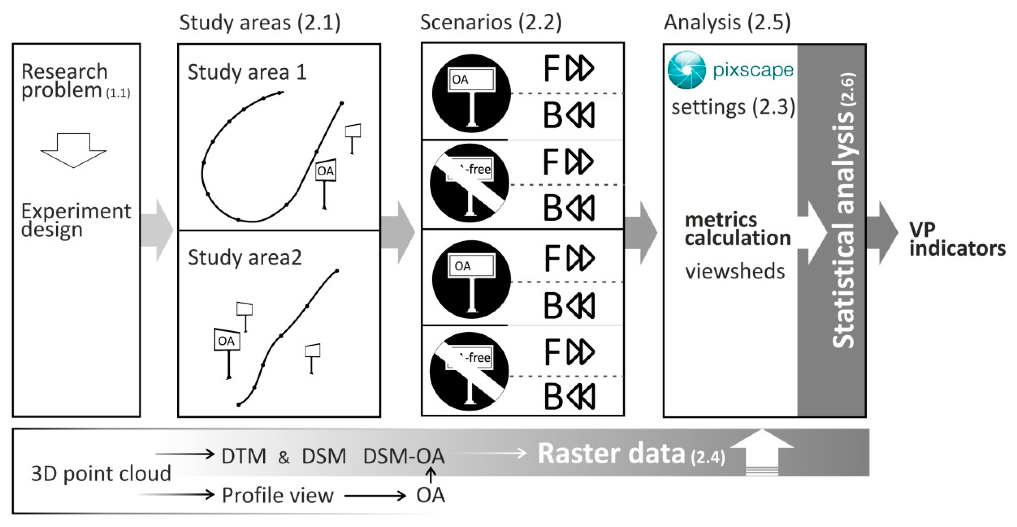
The method of measuring VP with the use of tangential view metrics consisted of several steps, which are graphically presented in Figure 1.
2.1. Study Areas
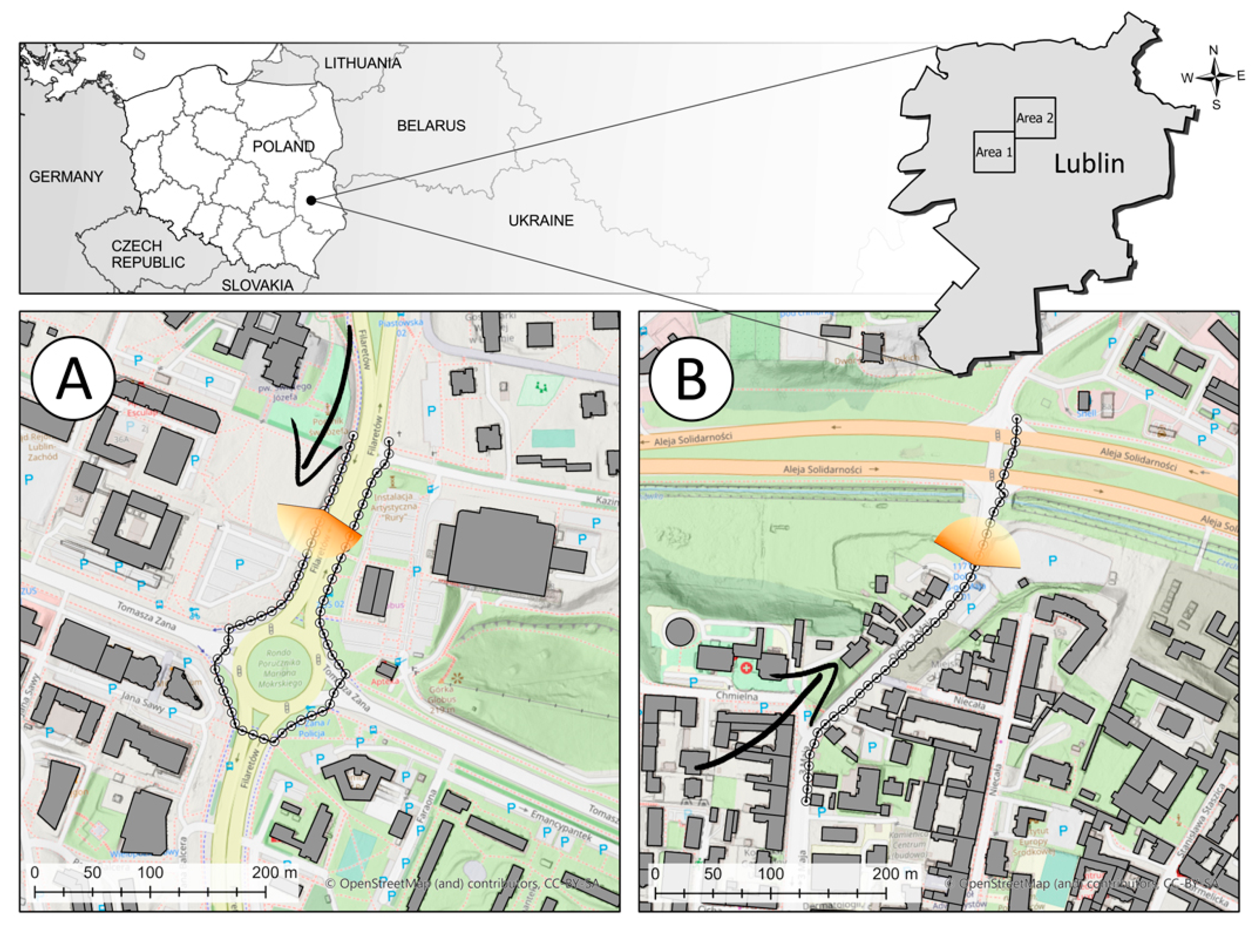
Experimentation occurred in the city of Lublin, Poland, one of the most dynamically developed cities in the country [72] where approximately 1037 OA are hosted by commercial agencies [73] (more OA are not officially inventoried). Lublin was selected for its diverse topography (terrain variations up to 70 m), which enables this type of experiment. To account for topographical environments as well as variation in the appearance of OA in Lublin’s urban landscape, two study areas with contrasting topographies were selected. Both sites were located in the city center and were spaced 4 km apart.
Centered on the T. Zana and Filaretów St. crossroads, Area 1 is relatively flat with elevation variations up to 4 m. Measurements for Area 1 were carried out along a 650 m pedestrian path, beginning at the Filaretów St. nearby the Saint Joseph church (Figure 2A). This path leads the observer southwards towards a roundabout where the highest concentrations of OA occur. The path follows the roundabout and loops northwards, where the VP caused by proliferation of OA gradually fades away. Buildings located approximately 100 m from the measurement path include skyscrapers.
Area 2 (Figure 2B) contains one of the steepest paths in the city; the Dolna 3-Maja St, with an 8% gradient. Measurements for Area 2 were carried out along a 450 m path, beginning at the medical clinic at Dolna 3-Maja St, the highest point of elevation (191.4 m) along the path. The path then moves towards the lowest point of elevation (176.9 m), located in the Czechówka river valley. During this gradual descent, the path is surrounded by three- or four-story buildings.
2.2. Experimental Scenarios
To simulate the visibility of the cityscape as experienced by an observer in motion, the pedestrian paths contained in Area 1 and Area 2 were digitized and observation points were established at 10 m intervals along each path. Each observation point was assigned a unique ID (from 1 to 66 in Area 1 and from 1 to 41 in Area 2). To investigate the influence of walking direction on visibility metric values, measurements were taken along each path in both the forwards (F) and backwards (B) directions relative to each path’s point of origin (Figure 2A,B). Thus, results are reported in relation to Area 1F, Area 1B, Area 2A, and Area 2B to indicate respective directions of motion.
Furthermore, the measurement of VP required some level of reference. For this, we considered a landscape without free-standing billboards to also be free of OA. As such, visibility metrics were first measured in OA-free scenarios. These measurements then served as reference data for subsequent measurements, which were repeated in the scenario with OA (OA scenario). Separate measurements were recorded for F and B directions in both OA-free and OA scenarios.
2.3. Viewpoint Range Parameters
A sequence of observation points as well as user-specified view range parameters are prerequisites for both tangential view and cumulative viewshed calculations. The space visible from a single vantage point is considered to be a single field of view (FoV). FoV sequences, cumulatively captured with each successive observation point, constitute a moving observer’s field of regard (FoR). The sum of viewed space in a FoR is therefore much larger than what is witnessed in a static FoV [74].
Human FoR consists of view zones in which varying degrees of detail recognition are possible. For example, the best detail recognition occurs in the central view zone (around 13 degrees), whereas detail recognition declines in the peripheral view zone at 107 degrees [75]. Furthermore, the visibility of space is influenced by the movement speed of a pedestrian as well as interactions with other pedestrians and behavior associated with wayfinding [76]. Lighting and weather also impose various influences on visibility. Thus, to account for the inherent heterogeneity of FoR, spatial extent generalization must be implemented and FoR parameters must be specified. The FoR parameters adopted for this experiment are outlined in the following paragraph.
The horizontal view angle was set to 160 degrees under the assumption that a cityscape observer looks around but does not rotate. As such, their horizontal FoR would be slightly wider than the 105 degrees [77] or 107 degrees if peripheral vision was included [75]. This constant value was maintained regardless of route direction changes and defined the directional nature of the analysis, which was contrary to a 360-degree approach [78]. The vertical FoR was constrained to +75 and −30 degrees. The lower value was reduced because the OA considered in this experiment did not occlude the lowest FoR zones. Thus, the exclusion of areas not related to this analysis was justified. The maximum viewing distance value was set to 500 m, which corresponds to a maximum distance of characteristic landscape feature recognition [79]. Additionally, a maximum viewing distance of 500 m ensured visibility analysis could extend to the borders of each study area. Finally, observer height was set up at 1.6 m above ground level, which corresponds to the average height of a European [23,80,81].
2.4. Digital Terrain Model (DTM) and Digital Surface Model (DSM) Rasters Processing Method (a 2.5D Landscape Model)
A digital terrain model (DTM) and a digital surface model (DSM) normalized to ground level constituted the source data for the 2.5D tangential view landscape metric calculations carried out in this experiment using PixScape software (v1.2) [68]. These 2D raster products were derived from a 3D point cloud, which was acquired at a point density of 12 points/m2 with the use of airborne laser scanning. The 3D point cloud was retrieved from the Polish National Geoportal [82] as classified LAS files (LAS 1.2 standard). Average point spacing was 0.2 m, which was dense enough to generate high-resolution raster products at a ground sampling distance (GSD) of 0.5 m. Ground points were filtered and converted to DTM raster file. All points classified as ground and building returns were used for the production of the DSM as well as points belonging to high and medium vegetation classes. To obtain height values referenced to ground level, the difference between the DSM and DTM was calculated using raster algebra. The product of this operation was the normalized DSM [83].
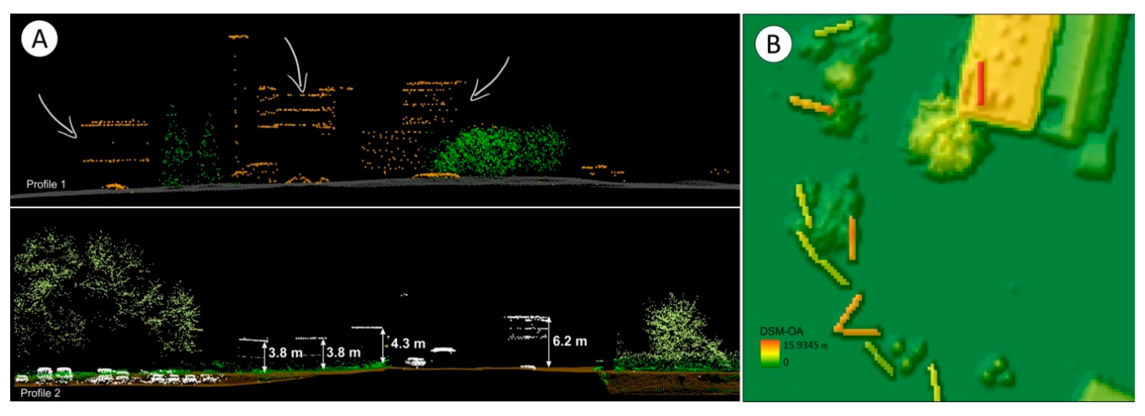
OA were identified in the profile view of the 3D point cloud. For this task, street view imagery was a useful supplement. Once identified, OA were manually digitized as linear features. In profile view, the height of each OA was measured from ground level to its upper edge and recorded as an attribute (Figure 3). The digitized OA were buffered to a distance of 0.5 m and converted to raster format with a spatial resolution of 0.5 m. Height attribute data were then assigned to corresponding pixel values.
To execute the OA scenario, the original DSM (described above) was modified with the addition of the OA raster, which encoded the spatial location and height of OA (this modified DSM will hereafter be referred to as DSM-OA, Figure 3B). To execute the OA-free scenario, the original DSM without OA was used. To reduce the edge effects inherent to 2.5D visualizations, mean focal statistics were calculated for DTM, DSM, DSM-OA within a 3 m circle radius. All rasters were saved as single-band TIFF files with the same spatial extent, resolution, and number of pixels (4000 × 4000 pixels).
2.5. Tangential View Metrics Method
The PixScape software enables the calculation of 11 tangential view metrics [68], each of which could provide insight for VP assessment. For this experiment, metrics referencing land use were excluded and only DTM- and DSM-dependent tangential view metrics were the object of further consideration. These metrics are Skyline (SL), Shannon depth (SD), and Depth line (DL) [48]. Additionally, this core set of tangential view metrics was supplemented with visible area metrics (Area) and maximum distance metrics (Dmax) due to their potential to characterize the VLC [34].
The SL metric is calculated as the ratio between the length of the skyline and that of the flat horizon line. Values for SL are close to one for the planar horizon, while higher values correspond to increasing skyline jaggedness [84]. In the context of visual pollution, it was assumed that the presence of OA in the cityscape would increase the value of the SL metric.
The SD metric corresponds to Shannon index applied to view depths which are grouped in four distance view classes: up to 10 m, from 10 to 100 m, from 100 m to 1000 m and above 1000 m [84]. In the context of visual pollution, it was assumed that the presence of OA in the cityscape would only decrease SD values under circumstances where several OA were located at a similar distance from the observer.
The DL metric is defined as an index of the compactness of a polygon that is bounded by points located at the farthest visible location from the observer [84]. In the context of visual pollution, it was assumed that the presence of OA in the cityscape would decrease DL values.
The Area metrics use square degrees to measure the visible area and therefore, the presence of OA in the cityscape was expected to increase the values of these metrics. The technical details of view sphere and square degree calculations are provided in PixScape software manual [84] as well as in Sahraoui et al. [48]. Pertinent to this research, the increasing number and size of vertical elements in the FoR reduce the impression of landscape openness [85]. As such, high values of Area metrics, measured at a given observation point, indicate landscape enclosure [86]. Conversely, areas of low visibility at 160-degree panoramic views indicate vast foreground and landscape openness. This allows for the analysis of the VP in the context of VLC. For the purpose of this experiment, the first and third quartiles of the Area metrics were calculated to indicate FoR with landscape openness and closure, respectively.
The Dmax metrics measure the line of sight distance to the farthest located visible pixel of tangential view [84]. It was assumed that the presence of OA may occlude distant views and therefore, a decrease in Dmax would be indicative of VP.
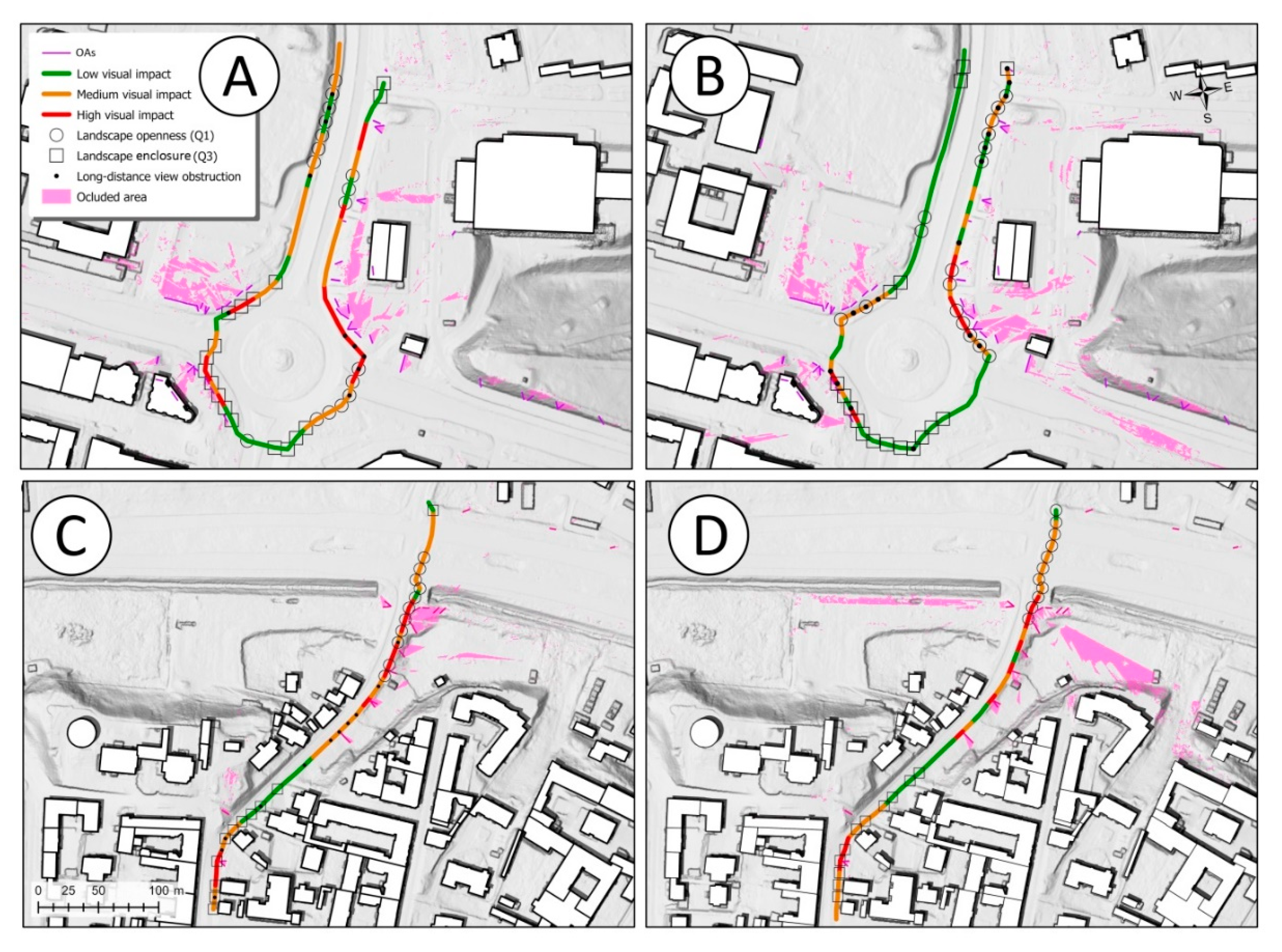
Metric values were calculated for all observation points in both the F and B directions. This was repeated for both the OA-free scenario and the OA scenario. All calculations were performed at default angular precision 0.1° [84]. The observer point locations and view range parameters were common for tangential visibility metrics as well as for cumulative viewshed analysis. The resulting metric values were the object of statistical analysis (Section 2.6) and interpretation regarding VP. Examples of tangential views were the object of visualization. Furthermore, to provide an example of cartographic visualization, a three-color scale has been adopted to indicate low, medium, and high visual impact along the measurement path. Green was assigned to the first quartile of metric values, yellow to the second, and red to the third. Thus, the presence (red) or absence (green) of VP phenomena in the analyzed cityscape are visualized, where the color orange represents what we propose to be a transition zone (details in Figure 6a–d).
2.6. Spatial and Statistical Analysis Methods
The experimental scenario results were compared (OA-free versus OA) to find statistically significant differences. We assumed that the presence of OA in the landscape would influence values of each of the tested metrics and that the level of achieved statistical significance will allow for the selection of metrics that are suitable for measuring VP phenomena regardless of the tested elevation conditions. The metric value distribution analysis for both the OA-free and the OA scenarios were performed independently for the F and B directions. The following basic statistical measures were used to compare both scenarios: median, minimum, and max value; first and third quartile; kurtosis; and the number of identical values. Statistical significance was tested with the use of Sign test and Wilcoxon non-parametric test at a p-value of 0.05. The Statistica (v 13.1) software was used for the above calculations.
The aim of the cumulative viewshed analysis was to quantify how much landscape area was visually occluded by OA. In other words, the cumulative viewshed analysis revealed what the observer, moving along each path, could not see due to the presence of OA in the cityscape. Calculating the occluded area facilitated a comparison between the occlusion effects experienced while traversing the F and B directions. This indicated which direction was more fragile to VP for each of the study areas.
To achieve this, the cumulative viewshed was calculated for both the OA-free scenario and OA scenarios. The resultant raster products were reclassified where visible pixels were assigned the value of 1 and non-visible pixels were assigned the value of 0. Raster algebra (a minus function) was applied to eliminate pixels that were visible in both scenarios. Thus, the product of the subtraction was a rasterized estimation of areas visually occluded by OA.
3. Results
3.1. Outdoor Advertisements and the Visibility Obstruction Effect.
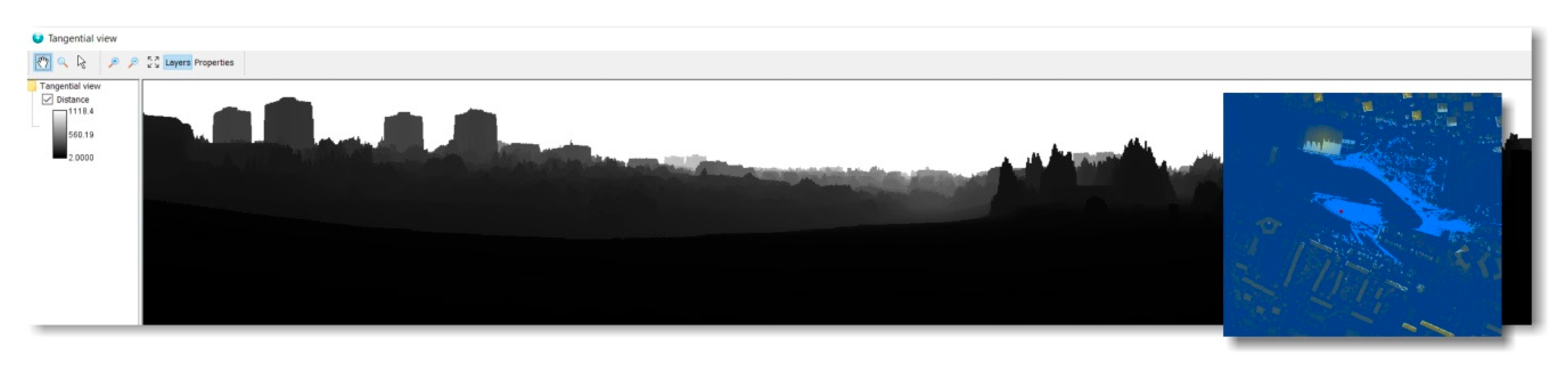
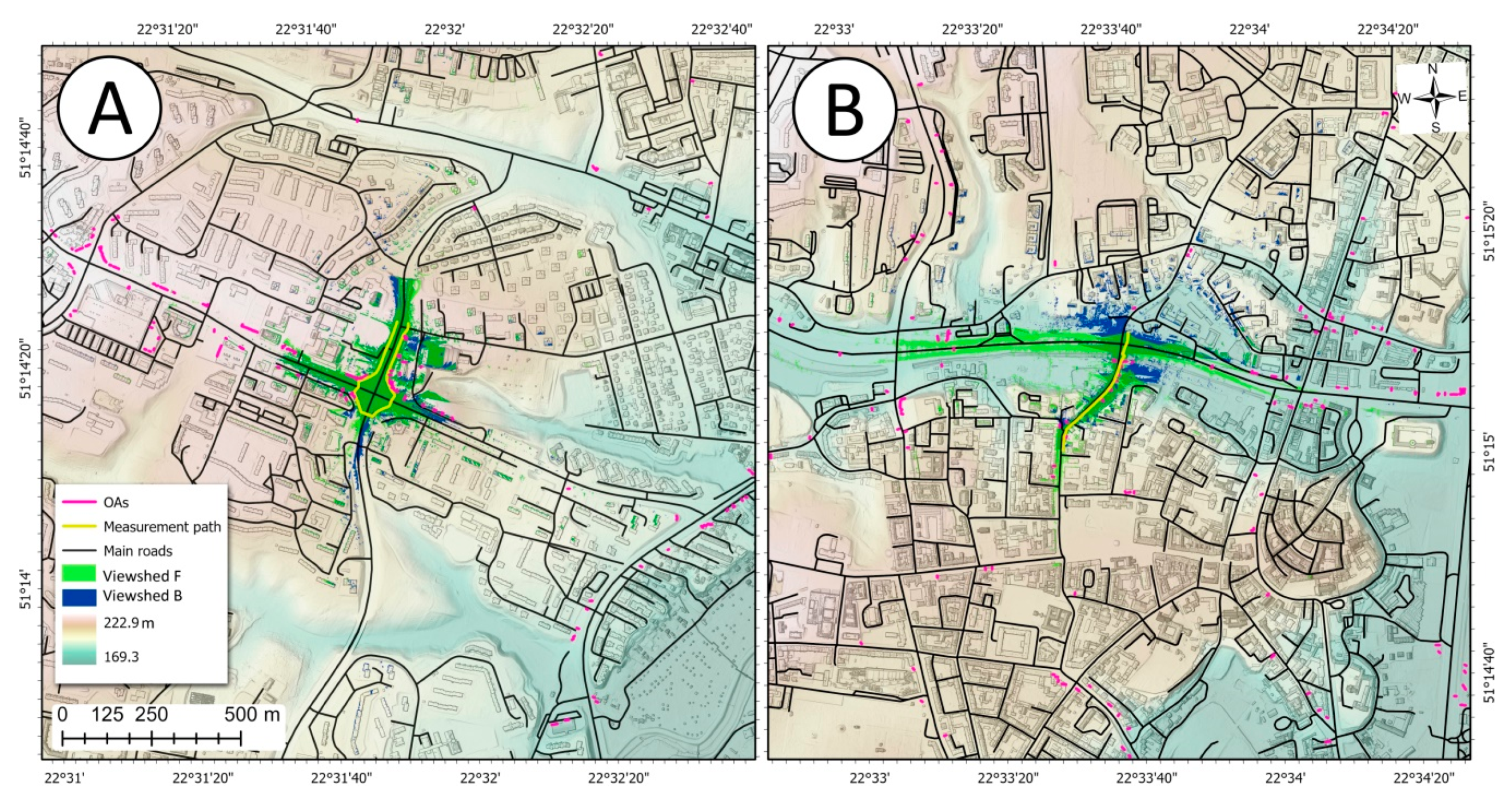
A total of 183 OA were located in Area 1. OA located on buildings were not included because these could not be differentiated from the buildings using the 2.5D technique. An example of the 2.5D view technique is presented in Figure 4. For the F direction, the cumulative viewshed area for the OA-free scenario was 8.48 ha. (Figure 5A). The presence of OA in the cityscape resulted in a visible area decrease of 8.06 ha. The obstructed visibility area, as a difference between the OA-free scenario and the OA scenario viewsheds, was 0.42 ha for the F direction. For the B direction the cumulative viewshed area for the OA-free scenario was 8.07 ha. The OA scenario resulted in a decrease to 7.53 ha, thus a slightly greater obstructed visibility area of 0.54 ha. The slightly larger obstructed visibility area in the B direction suggests that it was more susceptible to landscape damage than the F direction for Area 1. Measured view obstruction effect oscillated from 4.95% (F) to 6.70% (B) of the overviewed area depending on observer view directions.
A total of 233 OA were located in Area 2. The higher number of OA recorded here resulted from the fact that Area 2 was crossed by several main roads. It was at these intersections where OA were found to have proliferated. Despite the greater number of OA located in Area 2, its measurement path was 200 m shorter than that of Area 1 and runs through street frontage on both sides, which resulted in only 33 OA being visible from the path. The cumulative viewshed areas were 6.02 ha and 7.73 ha for the F and B directions, respectively (Figure 5B).
The presence of OA in the Area 2 resulted in a visible area decrease of 0.29 ha and 0.51 ha, for the F and B directions, respectively. This indicated that the view obstruction effect oscillated from 4.82% to 6.60% for the F and B directions, respectively. For Area 2, the VLC observed in the B direction appeared to be slightly more sensitive to the visibility occlusion effect (in both analyzed directions, the obstructed area did not exceed the 2% of the visible area.
3.2. Landscape Openness/Enclosure
In total, 5 tangential view metrics were subjected to statistical analysis with the goal of assessing their usefulness for measuring VP levels. As such, obtained values were interpreted in terms of VP. However, the Area metric is entitled to inference regarding landscape openness/enclosure and therefore, results pertaining to the VLC of measurement patches will be described first.
In the case of Area 1, the northern segment of the measurement path was characterized by landscape openness both in the F (Figure 6A) and B directions (Figure 6B). These points of openness were located far enough from dense, built-up areas to provide a wide, long-distance view. Additionally, a 50 m segment in F direction (from 380 m to 430 m) along the roundabout was classified as providing landscape openness. In the B direction, the segment spanning from 190 m to 230 m also provided landscape openness. The remaining southern parts along the roundabout were characterized as a landscape enclosure for both the F and B directions (with single openness exemption of pedestrian crossing providing a view of the road). This landscape enclosure was the result of high vegetation presence and a short proximity to buildings.
Trends in the location of landscape openness/enclosure within the Area 2 measurement path were similar in both the F (Figure 6C) and B directions (Figure 6D). The first segment (130 m in F direction) ran along street frontage and hence, the view from this segment was classified as a landscape enclosure. Continuing in the F direction, the path descended steeply towards the river valley (starting from 260 m) at which point VLS was open.
The instances of landscape openness and closure detailed above demonstrate unique vulnerabilities to VP. For instances of landscape openness, OA can easily become a dominant and disharmonious landscape feature. As for instances of landscape enclosure, OA can surpass tall vegetation and interior walls in a manner that likewise dominates the VLS. Both situations increase the effects of VP.
3.3. Tangential View Metrics
The basic statistics and non-parametric test results reported in this section were used to infer the usefulness and sensitivity of certain 2.5D tangential view metrics as VP indicators. As the focus of this research was the assessment of these metrics as VP indicators (presence/absence), the VP levels of each of the study areas are not compared in terms of more or less VP. To aid in the interpretation of the statistical outcomes described in this section, we direct the reader to the figures and tables.
Statistical summaries of the 2.5D tangential view metric results for Area 1 and Area 2 are provided in Table 1 and Table 2, respectively. These results are the product of the characterization of the full length of each respective measurement path. As the observation points were equally spaced at 10 m intervals, some results are referred to by measurement path location (m) rather than by point ID.
3.3.1. Area Metrics
For Area 1, the median and minimum as well as the first and third quartile values pertaining to the OA scenario were greater than those yielded from the OA-free scenario in both the F and B direction. The increase in values ranged from 28.11% to 5.44% points. The observed increase in the values of the minimum (8.15% and 15.49% for the F and B directions, respectively) and the first quartile (5.44% and 11.65% for the F and B directions, respectively) highlight the impact of OA on landscape openness. Kurtosis values were lower in the OA scenario than they were in the OA-free scenario. This was pronounced in the F direction. This lower concentration around the mean value of the Area metrics was attributed to the diffuse occurrence of VP phenomenon throughout the measurement path, which contained no local hot spots. These results indicated that the selected area metrics are good indicators of VP with the exception of the maximum area value, which showed no response to the presence of OA. This was because the maximum area value corresponded to a high wall of vegetation (located at 350 m) and not the presence of OA.
This unfavorable phenomenon is visualized in detail at Figure 6A. The highest VP concerns 20 m of landscape openness, the B direction (Figure 6B) results in 40 m of landscape openness affected by VP.
Of the 66 measurement points established in Area 1, only 6 did not respond to the presence of OA. While this was caused by the high concentration of OA in Area 1, it also validated the sensitivity of selected area metrics, distinguishing them as VP indicators. Moreover, this conclusion was confirmed by the results of the non-parametric tests, which reject the null hypothesis (p-value = 0.05) that the distribution of measurements for the OA and OA-free scenarios are equal.
As in Area 1, the median, minimum, as well as the first and third quartile values yielded from Area 2, were higher for the OA scenario than they were for the OA-free scenario. Likewise, the non-parametric tests confirmed a statistical difference between the OA and OA-free scenarios. These results verified the adequacy of the median, minimum, first quartile, and third quartile metrics as indicators of VP. The greater differences measured in the F direction (e.g., median increased by 4.56% and 2.14% for the F and B directions, respectively) indicated that this direction was more sensitive to VP direction. As with Area 1, VP measured in Area 2 concerns landscape openness (observation points 50 m for the F direction and 30 m for the B direction) and to a lesser extent, landscape enclosure (observation point 10 m for the F direction) (Figure 6C,D).
While higher in the OA scenario, the difference between metric values for the OA and OA-free scenarios in Area 2 was not as marked as observed for Area 1 (increases in values ranged from 0.02% points to 8.84% points). There were less OA in Area 2 than in Area 1 and not all measurement points showed changes in values. For example, the measurements reading at 9 points of the F direction and 12 for the B directions were the same in both scenarios.
3.3.2. Dmax Metrics
The non-parametric test results of the Dmax metrics did not prove to be statistically significant in all cases (Table 2). With regard to Area 1, the basic statistical results for Dmax metrics were less impressive compared to those of the Area metrics, which were proven to be statistically significant with the exception of Area maximum. Of the basic statistics used to describe the Dmax metric, decreases in the third quartile best indicated increases in VP with regard to long-distance views. The median, first quartile, and third quartile Dmax differences between the OA and OA-free scenarios for Area 1 ranged from 8.66% to 1.23%. The minimum and maximum values were unchanged. The Dmax metric has changed to the total number of 53 (F) and 49 (B) among 66 measurement points of Area 1. In the case of Area 2, only the F direction resulted in statistically significant differences (p-value = 0.002 and 0.003) for the Sign and Wilcoxson tests, respectively. In summary, the first quartile of the Dmax metric indicated that there was a significant distortion of the distant view detected in point 10 for F and 17 for B direction of Area 1 as well as in point 11 for F direction of Area 2. The location of these points within the VP zones is presented in Figure 6A–C.
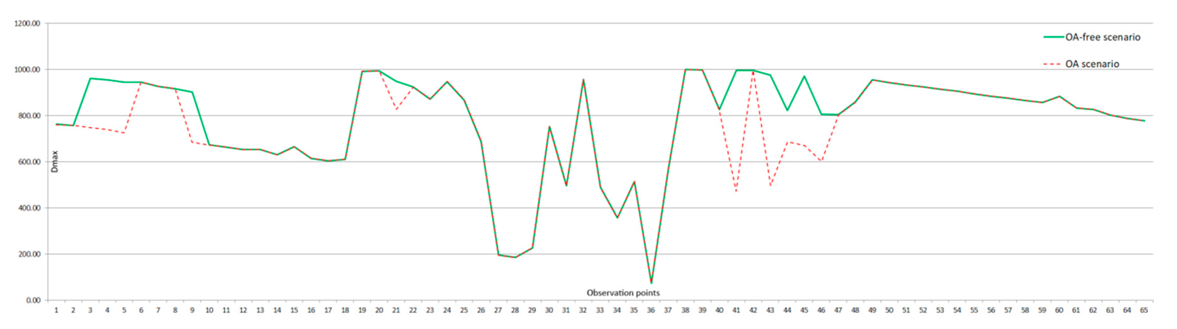
Despite these results, the Dmax metric turned out to be extremely valuable for VP diagnostics with some exceptions arising from the uphill slope of Area 2 in the B direction, which occluded long-distance views. As Dmax measures the distance to the farthest located visible pixel of the 2.5D landscape model, its values only changed when OA happened to obstruct the line of sight to the farthest located pixel. Therefore, Dmax was found to be a very selective indicator of VP. Instances of VP indication are visualized in Figure 7, where the Dmax curves for the OA and OA-free scenarios diverge.
3.3.3. The SL Metric
The Sign and Wilcoxson test results showed that the SL metric only functioned as a VP indicator in the case of relatively flat areas. As such, results for Area 2 were not statistically significant (Table 2). There are two explanations for this. First, while travelling uphill, the observer’s view of the skyline is occluded by terrain and thus, advertisement does not interfere with the skyline. Second, while travelling downhill, the observer views OA as features located below the skyline, which under these circumstances, do not affect landscape visibility. Generally speaking, however, SL values were found to increase in response to OA in the relatively flat and open landscape of Area 1.
The basic statistics for Area 1 ranged from 3.23% to 15.2% between scenarios. The directional influence on SL was difficult to interpret. However, using the first quartile as a primary indicator of directional effect, the B direction for Area 1 seemed to be more sensitive to skyline distortion caused by OA. At observation points where the visible skyline was relatively flat, first quartile values changed more significantly for the B direction rather than for the F direction (6.85% and 15.20% for F and B, respectively). Moreover, the increase in third quartile values for the F direction (15.64%) highlights the issue of a progressive complication of the skyline. In conclusion, the SL metric can be a good VP indicator dedicated to cityscapes with clearly distinguishable landmarks (e.g., church, tower), a situation in which the harmonious skyline shaped by landmarks is the object of landscape protection. Therefore, the SL can be recommended more for FoV rather than FoR analysis.
3.3.4. The SD and DL Metrics
With the exception of SD values for the F direction of Area 1 (p-values = 0.000016 and 0.000001 for the Sign and Wilcoxson tests, respectively), the SD and DL metrics did not pass the non-parametric tests. The SD metric uses four distance classes [84], which did not appear to be diverse enough to provide statistically significant results within the design of this experiment. While SD values for both the F and B directions varied between the OA and OA-free scenarios, there was no apparent trend to the oscillations of these values. This made clear interpretation impossible. The exception of significant results for SD values for the F direction suggests that this metric may operate randomly in VP indication and therefore cannot be recommended.
The DL results confirm that distance-dependent tangential view metrics are not a suitable measure of VP. The non-parametric test results did not provide any statistically significant differences between the two analyzed scenarios and therefore, the DL metrics cannot be recommended as VP indicators.
4. Discussion
The purpose of this research was to test selected visibility metrics as VP indicators. To do this, five tangential view metrics were assessed using basic statistics (median, minimum, maximum, Q1, and Q3) as well as non-parametric statistical tests (Sign and Wicoxson tests). Statistically significant results from the non-parametric tests proved Area and Dmax metrics to be useful indicators of VP. The area metric was found to be a good measure of general VP, while Dmax was found to indicate specific causes of visual disruption. Similarly, the selective usefulness of the SL metric was proven statistically significant by non-parametric tests. However, results indicate that the SL metric is best used for single FoV applications. The Area, Dmax, and SL metrics were all found to be directionally sensitive indicators, which demonstrated how the pedestrian perception of a cityscape may vary with their direction of movement. These findings are valuable as directional approaches to landscape research that address the human visual field of view are gaining traction in favor of generalized 360-degree analysis [87].
The metric values analyzed in this research were dependent on the source data for each study area and as such, were not described in detail (except in Table 1 and Table 2). Taking the Area metrics as an example, the degree to which landscapes are occluded is indicative of openness and not VP. Metrics should therefore be discussed in relation to specific land use classes. Otherwise, they only provide insight to VLC. However, mapping OA as a separate land use category for 2.5D tangential metrics calculations proved to be a challenging task. OA are relatively small and thin landscape features and are therefore difficult to distinguish in 2.5D. From a technical point of view, the DSM and the land use rasters would have to be compatible enough to ensure that OA pixels did not extend beyond the extruded DSM pixels so as to avoid OA spilling over onto the ground. The OA-free and OA scenarios then serve as a solution to this challenge. The difference between the two scenarios allows for the characterization of a particular land use class, which in this case is OA. However, it is not without further limitations. The 2.5D method excludes OA located on the facades of buildings as their tangent surfaces cannot be distinguished without 3D. This applies to store window advertising as well. Therefore, the case-study described here applies only to free-standing billboards. These technical limitations impede VP judgments, but do not mean that the 2.5D does not offer any solutions here. With regard to Area metrics, the VP judgements can be maintained if only the OA would be mapped on a building roof (or snapped to any tangential wall) instead of parallel to the facade. The Area metrics would then capture the increase in the visible area. This is a technical procedure, so it was not investigated in this work, but for VP measurements in areas where OA are located on buildings, such a technical modification is recommended
This approach enables further research on VP metrics as continuation of the work of Chmielewski [23] wherein the number of visible OA have been referenced with citizens’ subjective opinions on VP. The visible area metric and other visibility metrics can be analyzed in the same way to reveal thresholds for VP tolerance in relation to OA. The study of VP can be extended to metrics like degree of aggregation or fragmentation and texture [47]. However, this will only be possible when raster land use data that includes OA as a class is integrated into 2.5D analysis. Theoretically, VP could also be investigated with the use of visual complexity theory, which uses regularity and heterogeneity of a number of elements to measure a perceived complexity value and reference it to image evaluation by a group of humans [88]. Visual complexity theory has so far been applied in art object aesthetic evaluation [89] as well as advertising content design analysis [90]. Using the findings of Berlyne [91] as an analogy, who argued that an image becomes unattractive as the optimal level of complexity is exceeded, the images of visually polluted landscapes could be analyzed in the same manner. Theoretically, using image complexity metrics like fractal dimension, or spatial frequency [92], the threshold at which VP emerges could possibly be estimated. However, these considerations require empirical evidence.
Despite the fact that this research assesses the landscape threads of VP in terms of spatial chaos, the term of “chaos” should not be strictly evaluated as being negative. For example, spatial chaos as a feature of a cityscape’s unpredictability, can make the experience of traversing a city attractive. Furthermore, for subvertisers [93], who expect incompatibility, contestation, excess, and the dysfunctional in urban expression, OA emerge as sources of inspiration and (self)transformation [94]. From this perspective, the ordered and predictable city becomes unattractive, while for landscape architects who strive for harmonious and aesthetic spatial forms, the VP emerges as an unfavorable phenomenon affecting visual comfort and VLC. What these opposite approaches have in common is consent to the profanation of public space. The former use chaos as a form of communication [94]. The latter quantifies the landscape to propose sustainable solutions against spatial chaos [5,11,23] However, spatial chaos should not be confused with spatial uniformity [95]. As mentioned, the attribution of positive or negative qualities to spatial chaos depends on the personal aesthetics and education of the observer, and may be further influenced by experiencing the landscapes of branded-cities [96] in everyday life. Thus, some accept spatial chaos and try to give it a new meaning by finding their place within it. Others reject spatial chaos and escape to the uniformity of the suburbs where they can live closer to “nature”, which (surprisingly) contributes to the chaos of urban sprawl at larger scales. The latter put aesthetic needs forward because “chaos without a hint of connection is never pleasurable” [97]. It is to the former that this research is dedicated to.
5. Conclusions
Chaos is associated with something immeasurable. Therefore, environmental sciences have preferred other terms to address issues of system uncertainty, like the aforementioned entropy. Entropy in relation to landscape is associated with an increasing disorder of spatial features and the resulting perceptual–conceptual chaos [98]. For this reason, spatial chaos is equated with the phenomenon of VP.
Contrary to the field of urban studies, which synonymizes spatial chaos with a spatial disorder, some people may regard certain kinds of chaos as order [99]. This perspective depends on personal aesthetics, which in turn are influenced by art education. This brings forth the need to define spatial order against the hierarchical pattern of visual landscape priorities and objectives [100]. Defined landscape quality priorities can be evaluated with the use of landscape metrics derived from Shannon’s information theory (entropy). Such evaluation allows for the management of spatial chaos. To this end, the methods presented in this research may be implemented.
In summary, we have identified land use independent metrics as good indicators of VP, the limitations of which have been recognized. Despite the aforementioned technical limitations, it was statistically proven that particular metrics, to a greater or lesser extent, identify the presence of advertising chaos. As such, these metrics provide tools with which the spatially chaotic phenomenon of visual pollution may begin to be compartmentalized and understood.
Funding
The research was funded by the Ministry of Science and Higher Education (Poland) for the dissemination of science (766/P-DUN/2019).
Conflicts of Interest
The author declares no conflict of interest.
References
- Maslow, A.H.A. Theory of Human Motivation. Psychol. Rev. 1943, 50, 370–396. [Google Scholar] [CrossRef] [Green Version]
- McDermid, C.D. How money motivates men. Bus. Horiz. 1960, 3, 93–100. [Google Scholar] [CrossRef]
- Desmet, P.; Fokkinga, S. Beyond Maslow’s Pyramid: Introducing a Typology of Thirteen Fundamental Needs for Human-Cantered Design. Multimodal Technol. Interact. 2020, 4, 38. [Google Scholar] [CrossRef]
- Voronych, Y. Visual pollution of urban space in Lviv. Space Form. 2013, 20, 309–314. [Google Scholar]
- Szczepańska, M.; Wilkaniec, A.; Škamlová, L. Visual pollution in natural and landscape protected areas: Case studies from Poland and Slovakia. Quaest. Geogr. 2019, 38, 133–149. [Google Scholar] [CrossRef] [Green Version]
- Hasna, R.A.; Ajeeb, M.K. The Design of 3D Billboards Advertising in Jeddah, Saudi Arabia. Intern. Des. J. 2020, 10, 191–199. Available online: https://digitalcommons.aaru.edu.jo/faa-design/vol10/iss2/15 (accessed on 10 November 2020).
- Śleszyński, P.; Kowalewski, A.; Markowski, T.; Legutko-Kobus, P.; Nowak, M. The Contemporary Economic Costs of Spatial Chaos: Evidence from Poland. Land 2020, 9, 214. [Google Scholar] [CrossRef]
- Fry, G.; Tveit, M.S.; Ode, Å.; Velarde, M.D. The ecology of visual landscapes: Exploring the conceptual common ground of visual and ecological landscape indicators. Ecol. Indic. 2009, 9, 933–947. [Google Scholar] [CrossRef]
- Robert, S. Assessing the visual landscape potential of coastal territories for spatial planning. A case study in the French Mediterranean. Land Use Policy 2018, 72, 138–151. [Google Scholar] [CrossRef]
- Uuemaa, E.; Antrop, M.; Roosaare, J.; Marja, R.; Mander, Ü. Landscape metrics and indices: An overview of their use in landscape research. Living Rev. Landsc. Res. 2009. [Google Scholar] [CrossRef]
- Portella, A. Visual Pollution: Advertising, Signage and Environmental Quality; Ashgate Publishing: Farnham, UK, 2014. [Google Scholar]
- Boştină-Bratu, B.; Negoescu, A.G.; Palea, L. Consumer Acceptance of Outdoor Advertising: A Study of Three Cities. Land Forces Acad. Rev. 2018, 23. [Google Scholar] [CrossRef] [Green Version]
- Kamičaitytė-Virbašienė, J.; Godienė, G.; Kavoliūnas, G. Methodology of Visual Pollution Assessment for Natural Landscapes. J. Sustain. Archit. Civ. Eng. 2016, 13. [Google Scholar] [CrossRef] [Green Version]
- Drigo, M.O. Cidade/Invisibilidade e Cidade/Estranhamento: São Paulo Antes e Depois da lei “Cidade Limpa”. Galáxia 2009, 17, 49–64. Available online: https://revistas.pucsp.br/galaxia/article/view/2097 (accessed on 20 October 2020).
- Gomez, J.E.A. The Billboardization of Metro Manila. Int. J. Urban Reg. Res. 2013, 37, 186–214. [Google Scholar] [CrossRef]
- Tajuddin, S.N.A.A.; Zulkepli, N. An investigation of the use of language, social identity and multicultural values for nation-building in Malaysian outdoor advertising. Soc. Sci. 2019, 8, 18. [Google Scholar] [CrossRef] [Green Version]
- Motamed, B.; Farahani, L.; Jamei, E. Investigating the issue of pollution in the micro-scale design of mega- cities: A case study of Enghelab Street, Tehran. Manag. Res. Pract. 2015, 7, 43–59. [Google Scholar]
- Allahyari, H.; Salehi, E.; Zebardast, L. Evaluation of Visual Pollution in Urban Squares Using SWOT, AHP, and QSPM Techniques (Case Study: Tehran Squares of Enghelab and Vanak). J. Pollut. 2017, 3, 655–667. [Google Scholar]
- Karami, S.; Taleai, M. An Innovative Three-Dimensional Approach for Visibility Assessment of Highway Signs Based on the Simulation of Traffic Flow. J. Spat. Sci. 2020, 1–15. [Google Scholar] [CrossRef]
- Dymna, E.; Rutkiewicz, M. Polish Outdoor; Klucze Press: Warsaw, Poland, 2009. [Google Scholar]
- Madleňák, R.; Hudák, M. Analysis of data needs and having for the integrated urban freight transport management system. Commun. Comput. Inf. Sci. 2016, 40, 135–148. [Google Scholar] [CrossRef]
- Płuciennik, M.; Heldak, M. Outdoor Advertising in Public Space and its Legal System in Poland over the Centuries. IOP Conf. Ser. Mater. Sci. Eng. 2019, 471. [Google Scholar] [CrossRef]
- Chmielewski, S.; Lee, D.; Tompalski, P.; Chmielewski, T.J.; Wężyk, P. Measuring visual pollution by outdoor advertisements in an urban street using intervisibilty analysis and public surveys. Int. J. Geogr. Inf. Sci. 2016, 30, 801–818. [Google Scholar] [CrossRef]
- Chmielewski, S.; Samulowska, M.; Lupa, M.; Lee, D.; Zagajewski, B. Citizen science and WebGIS for outdoor advertisement visual pollution assessment. Comput. Environ. Urban Syst. 2018, 67, 97–109. [Google Scholar] [CrossRef]
- Chalkias, C.; Petrakis, M.; Psiloglou, B.; Lianou, M. Modelling of light pollution in suburban areas using remotely sensed imagery and GIS. J. Environ. Manag. 2006, 79, 57–63. [Google Scholar] [CrossRef] [PubMed]
- Falchi, F.; Cinzano, P.; Elvidge, C.D.; Keith, D.M.; Haim, A. Limiting the impact of light pollution on human health, environment and stellar visibility. J. Environ. Manag. 2011, 92, 2714–2722. [Google Scholar] [CrossRef] [PubMed]
- Ahmed, N.; Islam, M.N.; Tuba, A.S.; Mahdy, M.R.C.; Sujauddin, M. Solving visual pollution with deep learning: A new nexus in environmental management. J. Environ. Manag. 2019, 248, 109253. [Google Scholar] [CrossRef]
- Eyenga, I.I.; Focke, W.W.; Prinsloo, L.C.; Tolmay, A.T. Photodegradation: A solution for the shopping bag “visual pollution” problem? Macromol. Symp. 2002, 178, 139–152. [Google Scholar] [CrossRef]
- Elena, E.; Cristian, M.; Suzana, P. Visual pollution: A new axiological dimension of marketing? Ann. Fac. Econ. 2012, 1, 820–826. [Google Scholar]
- Kolláth, Z.; Száz, D.; Kolláth, K.; Tong, K.P. Light Pollution Monitoring and Sky Colours. J. Imaging 2020, 6, 104. [Google Scholar] [CrossRef]
- Enache, E.; Morozan, C.; Purice, S. Visual Pollution: A New Axiological Dimension of Marketing. In Proceedings of the 8th Edition of the International Conference “European Integration—New Challenges” EINCO2012, Oradea, Romania, 25–26 May 2012; pp. 2046–2051. Available online: http://anale.steconomiceuoradea.ro/volume/2012/proceedings-einco-2012.pdf (accessed on 10 September 2020).
- Jana, M.K.; De, T. Visual Pollution Can Have a Deep Degrading Effect on Urban and Sub-Urban Community: A Study in Few Places of Bengal, India, With Special Reference to Unorganized Billboards. Eur. Sci. J. 2015, 7881, 1–14. [Google Scholar]
- Madleňák, R.; Madleňáková, L.; Hoštáková, D.; Drozdziel, P.; Török, A. The Analysis of the Traffic Signs Visibility during Night Driving. Adv. Sci. Technol. Res. J. 2018, 12, 71–76. [Google Scholar] [CrossRef]
- Tveit, M.S. Landscape assessment in metropolitan areas—Developing a visual indicator-based approach. SPOOL 2014, 1, 301–316. [Google Scholar] [CrossRef]
- Tveit, M.; Ode, Å.; Fry, G. Key concepts in a framework for analysing visual landscape character. Landsc. Res. 2007, 31, 229–255. [Google Scholar] [CrossRef]
- Wakil, K.; Naeem, M.A.; Anjum, G.A.; Waheed, A.; Thaheem, M.J.; ul Hussnain, M.Q.; Nawaz, R. A Hybrid Tool for Visual Pollution Assessment in Urban Environments. Sustainability 2019, 11, 2211. [Google Scholar] [CrossRef] [Green Version]
- Nowghabi, A.S.; Talebzadeh, A. Psyhological Influence of Advertising Billboards on City Sight. Civ. Eng. J. 2019, 5, 390–397. [Google Scholar] [CrossRef] [Green Version]
- Bakar, S.A.; Al-Sharaa, A.; Maulan, S.; Munther, R. Measuring Visual Pollution Threshold along Kuala Lumpur Historic Shopping District Streets Using Cumulative Area Analysis. Vis. Resour. Steward. Conf. 2019, 16, 1–14. [Google Scholar]
- Bedin, B.; Ferrari, M.; Gajardo, R. A Poluição Visual e o Seu Controle No Município de Caxias Do Sul a Partir Da Lei Municipal No. 412/2012. Rev. Direito Cid. 2015, 7, 1708–1749. [Google Scholar] [CrossRef] [Green Version]
- Cercleux, A.-L.; Merciu, F.-C.; Merciu, G.-L. A Model of Development Strategy Encompassing Creative Industries to Reduce Visual Pollution—Case Study: Strada Franceză, Bucharest’s Old City. Procedia Environ. Sci. 2016, 32, 404–411. [Google Scholar] [CrossRef] [Green Version]
- García Carrizo, J. Sustainable Outdoor Advertising in the Contemporary City. In Proceedings of the 6th International Conferences Creatives Cities, Orlando, FL, USA, 24–25 January 2018; pp. 252–269. [Google Scholar] [CrossRef]
- Aydin, C.C.; Nianci, R. Environmental Harmony and Evaluation of Advertisement Billboards with Digital Photogrammetry Technique and GIS Capabilities: A Case Study in the City of Ankara. Sensors 2008, 8, 3271–3286. [Google Scholar] [CrossRef]
- Uuemaa, E.; Mander, U.; Marja, R. Trends in the use of landscape spatial metrics as landscape indicators: A review. Ecol. Indic. 2013, 18, 100–106. [Google Scholar] [CrossRef]
- Tenerelli, P.; Püffel, C.; Luque, S. Spatial Assessment of Aesthetic Services in a Complex Mountain Region: Combining Visual Landscape Properties with Crowdsourced Geographic Information. Landsc. Ecol. 2017, 32, 1097–1115. [Google Scholar] [CrossRef]
- Bartie, P.; Reitsma, F.; Kingham, S.; Mills, S. Advancing Visibility Modelling Algorithms for Urban Environments. Comput. Environ. Urban Syst. 2010, 34, 518–531. [Google Scholar] [CrossRef]
- Bowman, D.A.; McMahan, R.P. Virtual reality: How much immersion is enough? Computer 2007, 40, 36–43. [Google Scholar] [CrossRef]
- Sahraoui, Y.; Clauzel, C.; Foltête, J.C. Spatial Modelling of Landscape Aesthetic Potential in Urban-Rural Fringes. J. Environ. Manag. 2016, 181, 623–636. [Google Scholar] [CrossRef] [PubMed]
- Sahraoui, Y.; Youssoufi, S.; Foltête, J.C. A Comparison of in situ and GIS Landscape Metrics for Residential Satisfaction Modeling. Appl. Geogr. 2016, 74, 199–210. [Google Scholar] [CrossRef]
- Youssoufi, S.; Houot, H.; Vuidel, G.; Pujol, S.; Mauny, F.; Foltête, J.C. Combining Visual and Noise Characteristics of a Neighbourhood Environment to Model Residential Satisfaction: An Application Using GIS-Based Metrics. Landsc. Urban Plan. 2020, 204, 103932. [Google Scholar] [CrossRef]
- Karasov, O.; Heremans, S.; Külvik, M.; Domnich, A.; Chervanyov, I. On How Crowdsourced Data and Landscape Organisation Metrics Can Facilitate the Mapping of Cultural Ecosystem Services: An Estonian Case Study. Land 2020, 9, 158. [Google Scholar] [CrossRef]
- Jean-Christophe, F.; Jens, I.; Nicolas, B. Coupling Crowd-Sourced Imagery and Visibility Modelling to Identify Landscape Preferences at the Panorama Level. Landsc. Urban Plan. 2020, 197, 103756. [Google Scholar] [CrossRef]
- Hilal, M.; Joly, D.; Roy, D.; Vuidel, G. Visual Structure of Landscapes Seen from Built Environment. Urban For. Urban Green. 2018, 32, 71–80. [Google Scholar] [CrossRef] [Green Version]
- Lee, K.Y.; Seo, J.I.; Kim, K.-N.; Lee, Y.; Kweon, H.; Kim, J. Application of Viewshed and Spatial Aesthetic Analyses to Forest Practices for Mountain Scenery Improvement in the Republic of Korea. Sustainability 2019, 11, 2687. [Google Scholar] [CrossRef] [Green Version]
- Niedźwiecka-Filipiak, I.; Rubaszek, J.; Podolska, A.; Pyszczek, J. Sectoral Analysis of Landscape Interiors (SALI) as One of the Tools for Monitoring Changes in Green Infrastructure Systems. Sustainability 2020, 12, 3192. [Google Scholar] [CrossRef] [Green Version]
- Chmielewski, T.J. Zmierzając ku Ogólnej Teorii Systemów Krajobrazowych. Probl. Ekol. Kraj. 2014, 21, 1–16. Available online: http://paek.ukw.edu.pl/pek/index.php/PEK/article/view/3131 (accessed on 8 July 2020).
- Nohl, W. Sustainable Landscape Use and Aesthetic Perception. Landsc. Urban Plan. 2001, 54, 223–237. [Google Scholar] [CrossRef]
- Antrop, M. Why Landscapes of the Past Are Important for the Future. Landsc. Urban Plan. 2005, 70, 21–34. [Google Scholar] [CrossRef]
- Papadimitriou, F. Modelling indicators and indices of landscape complexity: An approach using G.I.S. Ecol. Indic. 2002, 2, 17–25. [Google Scholar] [CrossRef]
- Hermes, J.; Van Berkel, D.; Burkhard, B.; Plieninger, T.; Fagerholm, N.; von Haaren, C.; Albert, C. Assessment and Valuation of Recreational Ecosystem Services of Landscapes. Ecosyst. Serv. 2018, 31, 289–295. [Google Scholar] [CrossRef]
- Solon, J.; Pomianowski, W. GraphScape—A new tool for analysing landscape spatial structure and connectivity. Probl. Ekol. Kraj. 2014, 38, 15–32. [Google Scholar]
- Nowosad, J.; Stepinski, T.F. Information Theory as a Consistent Framework for Quantification and Classification of Landscape Patterns. Landsc. Ecol. 2019, 34, 2091–2101. [Google Scholar] [CrossRef] [Green Version]
- Vranken, I.; Baudry, J.; Aubinet, M.; Visser, M.; Bogaert, J. A Review on the Use of Entropy in Landscape Ecology: Heterogeneity, Unpredictability, Scale Dependence and Their Links with Thermodynamics. Landsc. Ecol. 2015, 30, 51–65. [Google Scholar] [CrossRef] [Green Version]
- Wang, C.; Zhao, H. Spatial Heterogeneity Analysis: Introducing a New Form of Spatial Entropy. Entropy 2018, 20, 398. [Google Scholar] [CrossRef] [Green Version]
- McGarigal, K.; Cushman, S.A.; Ene, E. FRAGSTATS v4: Spatial Pattern Analysis Program for Categorical and Continuous Maps. Computer Software Program Produced by the Authors at the University of Massachusetts, Amherst. 2012. Available online: http://www.umass.edu/landeco/research/fragstats/fragstats.html (accessed on 14 August 2020).
- Adamczyk, J.; Tiede, D. ZonalMetrics—A Python Toolbox for Zonal Landscape Structure Analysis. Comput. Geosci. 2017, 99, 91–99. [Google Scholar] [CrossRef]
- Lustig, A.; Stouffer, D.; Roigé, M.; Worner, S. Towards more predictable and consistent landscape metrics across spatial scales. Ecol. Indic. 2015, 57, 11–21. [Google Scholar] [CrossRef]
- Mantey, D.; Pokojski, W. New Indicators of Spatial Chaos in the Context of the Need for Retrofitting Suburbs. Land 2020, 9, 276. [Google Scholar] [CrossRef]
- Sahraoui, Y.; Vuidel, G.; Joly, D.; Foltête, J.C. Integrated GIS Software for Computing Landscape Visibility Metrics. Trans. GIS 2018, 22, 1310–1323. [Google Scholar] [CrossRef]
- Hamilton, J.L.; Gerald, J. Visual Pollution Study, a Report to the Citizens of Jacksonville; Jacksonville Community Council, Inc.: Jacksonville, FL, USA, 1985; Volume 4, pp. 1–23. Available online: https://digitalcommons.unf.edu/jcci/4 (accessed on 5 December 2020).
- Nessim, A.A.; Khodeir, L.M. Evaluating the Visual and Light Pollution from Outdoor Advertising in Egyptian Streets. J. Eng. Appl. Sci. 2020, 67, 789–808. [Google Scholar]
- Petřík, P.; Fanta, J.; Petrtýl, M. It Is Time to Change Land Use and Landscape Management in the Czech Republic. Ecosyst. Health Sustain. 2015, 1, 1–6. [Google Scholar] [CrossRef]
- PricewaterhouseCoopers Annual Rapport 2011. Available online: http://www.pwc.pl/pl/wielkie-miasta-polski/raport_Lublin_2011.pdf (accessed on 10 October 2020).
- Polish Outdoor Advertising Chamber of Commerce 2016. Available online: http://igrz.home.pl/RAPORT%20OOH%202016.pdf (accessed on 10 October 2020).
- Jang, W.; Shin, J.H.; Kim, M.; Kim, K. Human Field of Regard, Field of View, and Attention Bias. Comput. Methods Programs Biomed. 2016, 135, 115–123. [Google Scholar] [CrossRef] [PubMed]
- Younis, O.; Al-Nuaimy, W.; Alomari, M.H.; Rowe, F. A Hazard Detection and Tracking System for People with Peripheral Vision Loss Using Smart Glasses and Augmented Reality. Int. J. Adv. Comput. Sci. Appl. 2019, 10, 1–9. [Google Scholar] [CrossRef] [Green Version]
- Liu, M.; Nijhuis, S. Mapping Landscape Spaces: Methods for Understanding Spatial-Visual Characteristics in Landscape Design. Environ. Impact Assess. Rev. 2020, 82, 106376. [Google Scholar] [CrossRef]
- Simpson, M.J. Mini-Review: Far Peripheral Vision. Vision Res. 2017, 140, 96–105. [Google Scholar] [CrossRef]
- Vukomanovic, J.; Orr, B.J. Landscape Aesthetics and the Scenic Drivers of Amenity Migration in the New West: Naturalness, Visual Scale, and Complexity. Land 2014, 3, 390–413. [Google Scholar] [CrossRef] [Green Version]
- Van der Ham, R.J.M.; Iding, J.A. De Landschaps-Typologie Naar Visuele Kenmerken. Methodiek en Gebruik; Department of Landscape Architecture, Wageningen University: Wageningen, The Netherlands, 1971. [Google Scholar]
- Kułaga, Z.; Litwin, M.; Tkaczyk, M.; Palczewska, I.; Zajączkowska, M.; Zwolińska, D.; Krynicki, T.; Wasilewska, A.; Moczulska, A.; Morawiec-Knysak, A.; et al. Polish 2010 Growth References for School-Aged Children and Adolescents. Eur. J. Pediatr. 2011, 170, 599–609. [Google Scholar] [CrossRef] [PubMed] [Green Version]
- Schirpke, U.; Tasser, E.; Tappeiner, U. Predicting Scenic Beauty of Mountain Regions. Landsc. Urban Plan. 2013, 111, 1–12. [Google Scholar] [CrossRef]
- Polish National Geoportal. Available online: www.geoportal.gov.pl (accessed on 6 September 2020).
- Wang, Y.; Weinacker, H.; Koch, B.A. Lidar point cloud based procedure for vertical canopy structure analysis and 3D single tree modelling in forest. Sensors 2008, 8, 3938–3951. [Google Scholar] [CrossRef] [PubMed]
- PixScape Software User Manual 2019. Available online: https://sourcesup.renater.fr/www/pixscape/download/manual-en.pdf (accessed on 10 October 2020).
- Hayward, S.; Franklin, S. Perceived Openness-Enclosure of Architectural Space. Environ. Behav. 1964, 6, 37–52. [Google Scholar] [CrossRef]
- Stamps, A.E. Evaluating Enclosure in Urban Sites. Landsc. Urban Plan. 2001, 57, 25–42. [Google Scholar] [CrossRef]
- Yanru, H.; Masoudi, M.; Chadala, A.; Olszewska-Guizzo, A. Visual Quality Assessment of Urban Scenes with the Contemplative Landscape Model: Evidence from a Compact City Downtown Core. Remote Sens. 2020, 12, 3517. [Google Scholar] [CrossRef]
- Carballal, A.; Fernandez-Lozano, C.; Rodriguez-Fernandez, N.; Santos, I.; Romero, J. Comparison of Outlier-Tolerant Models for Measuring Visual Complexity. Entropy 2020, 22, 488. [Google Scholar] [CrossRef]
- Douchová, V. Birkhoff’s Aesthetic Measure. Auc. Philos. Hist. 2016, 2015, 39–53. [Google Scholar] [CrossRef]
- Pieters, R.; Wedel, M.; Batra, R. The Stopping Power of Advertising: Measures and Effects of Visual Complexity. J. Mark. 2010, 74, 48–60. [Google Scholar] [CrossRef]
- Berlyne, D. Novelty, complexity, and hedonic value. Percept. Psychophys. 1970, 8, 279–286. [Google Scholar] [CrossRef]
- Durmus, D. Spatial frequency and the performance of image-based visual complexity metrics. IEEE Access 2020, 8, 100111–100119. [Google Scholar] [CrossRef]
- Chung, S.K.; Kirby, M.S. Media Literacy Art Education: Logos, Culture Jamming, and Activism. Art Educ. 2009, 62, 34–39. [Google Scholar] [CrossRef]
- Dekeyser, T. Dismantling the Advertising City: Subvertising and the Urban Commons to Come. Environ. Plan. D Soc. Space 2020, 1–19. [Google Scholar] [CrossRef]
- Dekeyser, T. The material geographies of advertising: Concrete objects, affective affordance and urban space. Environ. Plan. A Econ. Space 2018, 50, 1425–1442. [Google Scholar] [CrossRef]
- Iveson, K. Branded Cities: Outdoor Advertising, Urban Governance, and the Outdoor Media Landscape. Antipode 2012, 44, 151–174. [Google Scholar] [CrossRef]
- Lynch, K. The Image of the City; The MIT Press: Cambridge, MA, USA, 1960. [Google Scholar]
- Oleński, W. Postrzeganie Krajobrazu Miasta w Warunkach Wertykalizacji Zabudowy. Ph.D. Thesis, Politechnika Krakowska, Kraków, Poland, 2014. Available online: https://repozytorium.biblos.pk.edu.pl/redo/resources/26294/file/suwFiles/OlenskiW_PostrzeganieKrajobrazu.pdf (accessed on 10 October 2020).
- Walter, J.A. Order and chaos in landscape. Landsc. Res. 1985, 10, 2–8. [Google Scholar] [CrossRef]
- Rombos, N.A. Aspects of Order and Chaos for the Cityscape; Syracuse University: New York, NY, USA, 1971; pp. 141–145. [Google Scholar]
Figure 1.
The methods flowchart. The research problem of measuring VP with the use of tangential view landscape metrics was examined on the example of two case study areas (2.1). The experiment scenario (2.2) assumed measurements in OA-free and OA scenarios, each time in both F and B directions of the case-study observation routes. The input data (2.4) were imported into Pixscape software (2.5) and the results were statistically evaluated (Section 2.6).

Figure 2.
The location of the study areas: (A) the first study area at Zana St., (B) the second study area at Dolna 3-Maja St, characterized by high height differences. The arrows indicate the F (forward) visibility analysis directions, view cones symbolize the adopted FoR (details in the method).
Figure 2.
The location of the study areas: (A) the first study area at Zana St., (B) the second study area at Dolna 3-Maja St, characterized by high height differences. The arrows indicate the F (forward) visibility analysis directions, view cones symbolize the adopted FoR (details in the method).

Figure 3.
The outdoor advertisements: (A) the digitalization on a profile view of 3D point cloud (a profile views delivered from LP360 Qcoherent software), (B) the example of a digital surface model (DSM)–OA raster.
Figure 3.
The outdoor advertisements: (A) the digitalization on a profile view of 3D point cloud (a profile views delivered from LP360 Qcoherent software), (B) the example of a digital surface model (DSM)–OA raster.

Figure 4.
The tangential view rendered by PixScpe software: The metric values were calculated in batch mode of PixScape software skipping the 2.5D tangential view rendering process. However, to explain the idea of tangential view and discuss some method limitations (Section 4 an example of 2.5D landscape visualizations results are given along with the observation point viewshed coverage (upper right).

Figure 5.
The OA location and the results of directional viewsheds modelling (green is forward direction, blue is backward): (A) Area 1, (B) Area 2.
Figure 5.
The OA location and the results of directional viewsheds modelling (green is forward direction, blue is backward): (A) Area 1, (B) Area 2.

Figure 6.
The results of VP measurement with the use of Area metrics, three-color grade refers to the visual impact of OA along the observation path: (A) the F directions of the study area 1, (B) the B direction of study area 1, (C) the F direction of study area 2, (D) the B direction of study area 2.

Figure 7.
Instances of VP obstruction in long distance views (graph visualization for the first study area, F direction).
Figure 7.
Instances of VP obstruction in long distance views (graph visualization for the first study area, F direction).


Table 1.
The tangential view landscape metrics of study area 1.
| Metrics | Median | Mini | Max | Q1 | Q3 | n/No Change | Kurtosis | Sign Test (p-Value) | Wilcoxon Test (p-Value) |
|---|---|---|---|---|---|---|---|---|---|
| Area, OAfree (F) | 2910.6 | 2269.8 | 11894.3 | 2723.8 | 3402.8 | 65/6 | 24.546 | 7.550957 | 6.679959 |
| Area, OA (F) | 3267.8 | 2454.9 | 11894.3 | 2872.1 | 4359.3 | 15.439 | (0.000000) | (0.000000) | |
| % point | 12.27% | 8.15% | 0.00% | 5.44% | 28.11% | ||||
| Area, OAfree (B) | 2883.0 | 2265.6 | 10584.8 | 2643.9 | 3452.7 | 65/4 | 13.922 | 7.747008 | 6.846313 |
| Area, OA (B) | 3443.0 | 2616.6 | 10584.8 | 2951.9 | 4040.0 | 8.499 | (0.000000) | (0.000000) | |
| % point | 19.42% | 15.49% | 0.00% | 11.65% | 17.01% | ||||
| DistMax, OAfree (F) | 858.0 | 73.3 | 999.3 | 664.6 | 943.4 | 65/53 | 2.086 | 3.175426 | 3.059412 |
| DistMax, OA (F) | 787.4 | 73.3 | 999.3 | 652.3 | 905.2 | 1.345 | (0.001496) | (0.002218) | |
| % point | −8.22% | 0.00% | 0.00% | −1.85% | −4.05% | ||||
| DistMax, OAfree (B) | 793.5 | 189.7 | 999.1 | 602.9 | 880.2 | 66/49 | 0.117 | 3.880570 | 3.621365 |
| DistMax, OA (B) | 724.8 | 189.7 | 999.1 | 590.2 | 869.4 | 0.081 | (0.000104) | (0.000293) | |
| % point | −8.66% | 0.00% | 0.00% | −2.11% | −1.23% | ||||
| SL, OAfree (F) | 1.963 | 1.599 | 3.445 | 1.809 | 2.212 | 65/12 | 0.154 | 6.249068 | 6.544095 |
| SL, OA (F) | 2.067 | 1.803 | 3.678 | 1.933 | 2.558 | 0.153 | (0.000000) | (0.00000) | |
| % point | 5.30% | 12.76% | 6.76% | 6.85% | 15.64% | ||||
| SL, OAfree (B) | 1.964 | 1.551 | 3.422 | 1.730 | 2.478 | 66/9 | 0.318 | 5.715006 | 6.264394 |
| SL_OA (B) | 2.200 | 1.607 | 3.560 | 1.993 | 2.558 | 0.566 | (0.000000) | (0.000000) | |
| % point | 12.02% | 3.61% | 4.03% | 15.20% | 3.23% | ||||
| SD, OAfree (F) | 0.783 | 0.184 | 0.999 | 0.562 | 0.914 | 65/14 | 0.555 | 4.314879 | 4.817665 |
| SD, OA (F) | 0.850 | 0.413 | 0.999 | 0.630 | 0.961 | 0.924 | (0.000016) | (0.000001) | |
| % point | 8.56% | 24.46 | 0.00% | 12.10% | 5.14% | ||||
| SD, OAfree (B) | 0.836 | 0.253 | 0.999 | 0.623 | 0.935 | 66/18 | 0.063 | 2.384158 | 2.848357 |
| SD, OA (B) | 0.860 | 0.317 | 0.999 | 0.694 | 0.932 | 0.081 | (0.017118) | (0.004395) | |
| % point | 2.87% | 25.30% | 0.00 | 11.40% | −0.32% | ||||
| DL, OAfree (F) | 17.445 | 4.712 | 33.600 | 13.463 | 21.587 | 65/6 | 0.074 | 0.260378 | 1.826610 |
| DL, OA (F) | 17.06 | 4.712 | 33.897 | 13.777 | 20.698 | 0.248 | (0.794572) | (0.067759) | |
| % point | −2.21% | 0.00% | 0.88% | 2.33% | −4.12% | ||||
| DL, OAfree (B) | 15.673 | 4.9310 | 40.421 | 10.410 | 19.546 | 66/4 | 2.544 | 0.127000 | 1.447787 |
| DL, OA (B) | 14.987 | 4.9776 | 40.421 | 10.890 | 18.221 | 3.611 | (0.898940) | (0.147678) | |
| % point | −4.38% | 0.95% | 0.00 | 4.61 | −6.78 |
Table 2.
The tangential view landscape metrics of study area 2.
| Metrics | Median | Mini | Max | Q1 | Q3 | n/No Change | Kurtosis | Sign Test (p-Value) | Wilcoxon Test (p-Value) |
|---|---|---|---|---|---|---|---|---|---|
| Area, OAfree (F) | 7384.6 | 5635.3 | 11579.5 | 5878.2 | 7955.4 | 41/9 | 0.831 | 5.480078 | 4.936520 |
| Area, OA (F) | 7721.5 | 5635.4 | 11579.5 | 6397.8 | 8211.4 | 0.707 | (0.000000) | (0.000001) | |
| % point | 4.56% | 0.00 | 0.00 | 8.84% | 3.22% | ||||
| Area, OAfree (B) | 8328.3 | 5842.3 | 10513.2 | 6582.9 | 8843.3 | 41/12 | −0.997 | 5.199469 | 4.703046 |
| Area, OA (B) | 8506.6 | 5843.2 | 10516.5 | 7159.7 | 8886.4 | −0.860 | (0.000000) | (0.000003) | |
| % point | 2.14% | 0.02% | 0.03% | 8.76% | 0.49% | ||||
| DistMax, OAfree (F) | 949.5 | 557.1 | 1000.2 | 837.1 | 980.5 | 41/30 | 0.630 | 3.015113 | 2.934058 |
| DistMax, OA (F) | 898.5 | 115.0 | 1000.2 | 712.9 | 965.2 | 3.213 | (0.002569) | (0.003346) | |
| % point | −5.37% | −79.36% | 0.00 | −14.84% | −5.37% | ||||
| DistMax, OAfree (B) | 273.6 | 94.881 | 1000.0 | 166.243 | 551.502 | 41/34 | −0.406195 | 2.267787 | 2.366432 |
| DistMax, OA (B) | 273.6 | 83.055 | 1000.0 | 148.000 | 465.893 | 0.028178 | (0.023342) | (0.017961) | |
| % point | 0.00% | −12.46% | 0.00% | −10.97% | −15.52% | ||||
| SL, OAfree (F) | 1.950 | 1.587 | 3.720 | 1.851 | 2.163 | 41/10 | 0.267 | 0.176777 | (0.00000 |
| SL, OA (F) | 1.998 | 1.583 | 3.850 | 1.852 | 2.156 | 0.575 | (0.859684) | (1.00000) | |
| % point | 2.46% | −0.25% | 3.49% | 0.05% | −0.32% | ||||
| SL, OAfree (B) | 1.772 | 1.551 | 3.531 | 1.691 | 1.995 | 41/19 | 0.082 | 1.485563 | 2.865074 |
| SL_OA (B) | 1.859 | 1.535 | 3.510 | 1.752 | 2.087 | −0.006 | (0.137395) | (0.004169) | |
| % point | 4.91 | −1.03 | −0.59 | 3.61 | 4.61 | ||||
| SD, OAfree (F) | 0.739 | 0.143 | 0.992 | 0.599 | 0.822 | 41/12 | 0.541 | 0.742781 | 1.286580 |
| SD, OA (F) | 0.718 | 0.143 | 0.997 | 0.565 | 0.838 | −0.043 | (0.457614) | (0.198241) | |
| % point | −2.84% | 0.00% | 0.50% | −5.68% | 1.95% | ||||
| SD, OAfree (B) | 0.697 | 0.093 | 0.994 | 0.406 | 0.780 | 41/16 | −0.735 | 0.400000 | 1.735496 |
| SD, OA (B) | 0.672 | 0.093 | 0.999 | 0.467 | 0.837 | −0.675 | (0.689157) | (0.082654) | |
| % point | −3.59% | 0.00% | 0.50% | 15.02% | 7.31% | ||||
| DL, OAfree (F) | 22.271 | 7.965 | 34.191 | 18.487 | 25.355 | 41/9 | −0.513 | 2.298097 | 2.917035 |
| DL, OA (F) | 19.629 | 7.965 | 32.588 | 16.150 | 22.519 | −0.714 | (0.021556) | (0.003534) | |
| % point | −11.86 | 0.00 | −4.69 | −12.64 | −11.19 | ||||
| DL, OAfree (B) | 9.069 | 5.421 | 30.716 | 7.356 | 14.050 | 41/12 | 2.354 | 0.742781 | 0.637884 |
| DL, OA (B) | 8.902 | 5.132 | 23.237 | 7.092 | 14.976 | −0.443 | (0.457614) | (0.523549) | |
| % point | −1.84 | −5.33 | −24.35 | −3.59 | 6.59 |
Publisher’s Note: MDPI stays neutral with regard to jurisdictional claims in published maps and institutional affiliations. |
© 2020 by the author. Licensee MDPI, Basel, Switzerland. This article is an open access article distributed under the terms and conditions of the Creative Commons Attribution (CC BY) license (http://creativecommons.org/licenses/by/4.0/).
Share and Cite
MDPI and ACS Style
Chmielewski, S. Chaos in Motion: Measuring Visual Pollution with Tangential View Landscape Metrics. Land 2020, 9, 515. https://0-doi-org.brum.beds.ac.uk/10.3390/land9120515
AMA Style
Chmielewski S. Chaos in Motion: Measuring Visual Pollution with Tangential View Landscape Metrics. Land. 2020; 9(12):515. https://0-doi-org.brum.beds.ac.uk/10.3390/land9120515
Chicago/Turabian StyleChmielewski, Szymon. 2020. "Chaos in Motion: Measuring Visual Pollution with Tangential View Landscape Metrics" Land 9, no. 12: 515. https://0-doi-org.brum.beds.ac.uk/10.3390/land9120515
Note that from the first issue of 2016, this journal uses article numbers instead of page numbers. See further details here.