
Rolling Cargo Management Using a Deep Reinforcement Learning Approach


1
Department of Computer Science, Jönköping University, 553 18 Jönköping, Sweden
2
Department of Pharmaceutical Biosciences, Uppsala University, 752 36 Uppsala, Sweden
3
Stena Line, 413 27 Göteborg, Sweden
4
Centre for Reliable Machine Learning, University of London, London WC1E 7HU, UK
*
Authors to whom correspondence should be addressed.
Logistics 2021, 5(1), 10; https://0-doi-org.brum.beds.ac.uk/10.3390/logistics5010010
Submission received: 27 November 2020
/
Revised: 28 January 2021
/
Accepted: 31 January 2021
/
Published: 8 February 2021
(This article belongs to the Special Issue Applications of AI and Machine Learning Models for Logistics and Supply Chain Management)
Abstract
:Loading and unloading rolling cargo in roll-on/roll-off are important and very recurrent operations in maritime logistics. In this paper, we apply state-of-the-art deep reinforcement learning algorithms to automate these operations in a complex and real environment. The objective is to teach an autonomous tug master to manage rolling cargo and perform loading and unloading operations while avoiding collisions with static and dynamic obstacles along the way. The artificial intelligence agent, representing the tug master, is trained and evaluated in a challenging environment based on the Unity3D learning framework, called the ML-Agents, and using proximal policy optimization. The agent is equipped with sensors for obstacle detection and is provided with real-time feedback from the environment thanks to its own reward function, allowing it to dynamically adapt its policies and navigation strategy. The performance evaluation shows that by choosing appropriate hyperparameters, the agents can successfully learn all required operations including lane-following, obstacle avoidance, and rolling cargo placement. This study also demonstrates the potential of intelligent autonomous systems to improve the performance and service quality of maritime transport.
1. Introduction
Intelligent transportation systems implement advanced technologies such as sensing, awareness, data transmission, and intelligent control technologies in mobility and logistics systems. For mobility, the objective is to increase transport performance and achieve traffic efficiency by minimizing traffic problems such as congestion, accidents, and resource consumption. The same goals are targeted for logistics, but the focus is on the optimization of resource consumption, cost, and time, as well as on the efficiency, safety, and reliability of logistic operations.
Smart ports have emerged as a new form of port that utilizes the Internet of Things, artificial intelligence, blockchain, and big data in order to increase the level of automation and supply chain visibility and efficiency. Digital transformation of ports, terminals, and vessels has the potential to redefine cross-border trade and increase shipping operation efficiency [1]. Orive et al. [2] gave a thorough analysis of the conversion to digital, intelligent, and green ports and proposed a new methodology, called the business observation tool, that allows successfully undertaking the automation of terminals considering the specific constraints of the port. Furthermore, various logistics operations have been studied using new techniques such as cargo management, traffic control, detection, recognition and tracking of traffic-related objects, and optimization of different resources such as energy, time, and materials [3,4]. The state-of-the-art of smart ports and intelligent maritime transportation has been described highlighting trends, challenges, new technologies, and their implementation status [5,6,7].
At the same time, the past few years have witnessed breakthroughs in reinforcement learning (RL). Some important successes were recorded, namely learning a policy from pixel input in 2013 [8], beating the world champion by AlphaGo Master [9], and the OpenAI Dexterity program in 2019 [10]. Reinforcement learning refers to goal-oriented algorithms, which learn how to attain a complex objective (goal) or how to maximize along a defined dimension over time. The agent interacts with its environment in discrete time steps. At each time step, the agent receives an observation, which typically includes the reward. Based on this feedback, the agent chooses an action from the set of available actions, which is subsequently sent to the environment. The environment state is changing, and the goal of the agent is to maximize its collected reward.
The objective of this paper is to assess the feasibility and efficiency of deep RL techniques (DRL) in teaching a multiagent system to accomplish complex missions in a dynamic constrained environment. Handling of rolling cargo in ports is an appropriate field to achieve this purpose, in which the agents can be autonomous tug masters and the environment reflects the real world. Our particular application is the automation of the loading and unloading of rolling cargo from ships. These two operations are essential and recurrent in maritime shipping and aim to move rolling cargo from the quay or defined points in the terminal to onboard ships. This kind of ship is called a roll-on/roll-off (RORO) ship. The optimization of these services will be of great benefit in terms of time, energy, space, service quality, etc. This paper focuses on the loading operation since it is the most challenging and has more constraints to meet.
This paper tries to provide approaches to practical challenges and answer the following research questions:
- How is the performance of the agents controlled by RL? We evaluate this by looking in particular at convergence and its speed, but also other metrics such as accumulative reward, episode length, and entropy.
- To what degree are the learned policies optimal? This will be analyzed by identifying if there are any emergent strategies that are not explicitly desired by the developer and that the tug masters have learned.
- What is the impact of tuning the learning hyperparameters on the quality of the achieved solution?
Our contribution consists of a DRL solution that simulates the handling of loading and unloading cargo using autonomous tug masters for RORO ships in smart ports. We evaluate the solution both regarding performance and policy optimality and can show that our system is able to solve the tasks included satisfactorily. We further assess the impact of different learning model hyperparameters on the quality of the solutions achieved. Our solution is also trained using incremental learning, adding additional challenges as the system learns to solve previously included tasks.
The remainder of this paper is organized as follows: The second section presents the related works and background theories of DRL. The third section provides the specifications of the autonomous system ensuring loading/unloading operations and describes the experimental setup. The obtained results are presented and analyzed in Section 4. Finally, conclusions are drawn in Section 5.
2. Background
2.1. Related Work
The use of machine learning techniques for cargo management has received considerable attention from researchers due to their achieved performance. Shen et al. [11] used a deep Q-learning network to solve the stowage planning problem and show the possibility to apply reinforcement learning for stowage planning. To perform an automated stowage planning in container ships, Lee et al. [12] provided a model to extract the features and to predict the lashing forces using deep learning without the explicit calculation of lashing force. The container relocation problem was solved using the random forest based branch pruner [13] and deep learning heuristic tree search [14]. This direction of research deals only with the management of cargo and particularly automated stowage planning and container relocation taking into consideration some logistic related constraints. Almost all these studies did not take into consideration the movement and operations required by cranes or autonomous vehicles in ports.
Another complementary track of research is the automation of cargo management using control and communication technologies. Price et al. [15] proposed a method to dynamically update the 3D crane workspace for collision avoidance during blind lift operations. The position and orientation of the crane load and its surrounding obstacles and workers were continuously tracked by 3D laser scanning. Then, the load swing and load rotation were corrected using a vision based detection algorithm to enhance the crane’s situational awareness and collision avoidance. Atak et al. [16] modeled quay crane handling time in container terminals using regression models and based on a big dataset of port operations and crane movements in Turkish ports.
Recently, attention has also been directed toward rolling cargo. M’hand et al. [17] proposed a real-time tracking and monitoring architecture for logistics and transport in RORO terminals. The system aims to manage dynamic logistics processes and optimize some cost functions such as traffic flow and check-in time. The specific mission of the system is the identification, monitoring, and tracking of the rolling cargo. Reference [18] discussed the potential evolution in the RORO industry that can be achieved by process mining in accordance with complex event processing. It gave an overview of process mining and complex event processing. It also introduced the RORO definition, subsystems, as well as the associated logistics processes. To take advantage of the autonomy capabilities, K. You et al. [19] proposed an automated freight transport system based on the autonomous container truck. The designed system operates in a dual-mode, mixing the autonomous driving, which is used in the terminal and connecting tunnels, with the manned driving mode, which is adopted within the operation area. One of the problems related to rolling cargo handling is the stowage problem in which the aim is to plan loading as much cargo as possible and maximizing the space utilization ratio on the decks, while respecting the time and reducing the cost spent on shifting cargo [20,21,22].
Machine learning based techniques are increasingly used to implement and automate the management of smart port services. The goal is to provide autonomy and increase the performance of the logistics operations. L. Barua et al. [7] reviewed the machine learning applications in international freight transportation management. In [23], the authors used RL for selecting and sequencing containers to load onto ships. The goal of this assignment task is to minimize the number of crane movements required to load a given number of containers with a specific order. Fotuhi et al. [24] proposed an agent based approach to solve the yard crane scheduling problem, which means determining the sequence of drayage trailers that minimizes their waiting time. The yard crane operators were modeled as agents using the Q-learning technique for automatic trailer selection process. In the same context, Reference [3] used the Q-learning algorithm to determine the movement sequence of the containers so that they were loaded onto a ship in the desired order. Their ultimate goal was to reduce the run time for shipping. As an extension of their work, they tried to optimize three processes simultaneously: the rearrangement order of containers, the layout of containers, assuring explicit transfer of the container to the desired position, and the removal plan for preparing the rearrangement operation [25].
In the unloading process, it is primordial to provide customers with precise information on when rolling cargo is available to be picked up by customers at the terminal. To fulfil this need, Reference [26] developed and tested a module based framework using statistical analysis for estimating the discharge time per cargo unit. The result achieved was the estimation of the earliest pick-up time of each individual truck or trailer within 1 h accuracy for up to 70% of all cargo. In [27], the authors proposed a simulation model to simulate the process of RORO terminal operations, in particular the entry and exit of vehicles, with the Arena software. The model also served to determine the scale of land parking lots to be assigned to RORO.
To the best of our knowledge, there is no work dealing with the autonomous management of these types of loading and unloading of rolling cargo using reinforcement learning. In addition, in our study, we consider both the stowage planning problem and the automation of tug master operations.
2.2. Deep Reinforcement Learning
Reinforcement learning (RL) is a branch of machine learning encompassing a set of techniques that try to learn the best agent strategy, called the policy, maximizing the reward functions of the agent. The policy, denoted by , is the way in which the agent chooses a specific action a on state s (called observation). Formally, the policy is a mapping from the state space to the action space, and it is generally stochastic. The environment is stochastic as well and can be modeled as a Markov decision process with state space S, action space A, transition dynamics , reward function , and a set of initial states [28]. Considering the agent objectives, trajectories can be extracted from the process by repeatedly sampling the agent’s action from its policy and the next state from . The total reward is the sum of each step’s reward and can be represented as .
To maximize the expected sum of rewards, a state-value function is defined to be the expected return from time t onwards with respect to and starting from the state s. It measures the quality of being in a specific state. Another important function is the action value function , which represents the expected return from time t onwards if an action is performed at state s. It measures the profitability of taking a specific action in a state s. The techniques that use these two functions are called value based RL. The objective of value based RL is to estimate the state-value function and then infer the optimal policy. In contrast, the policy gradient methods directly optimize the policy with respect to the expected return (long-term cumulative reward) by performing gradient ascent (or descent) on the policy parameters. The policy based methods are considered more efficient especially for high-dimensional or continuous action spaces.
To be able to optimize the policy using gradient based methods, the policy is assumed to be defined by some differentiable function , parameterized by . These methods use gradient ascent approximations to gradually adjust the policy parameterized function in order to optimize the long-term return according to the approximation . is the policy gradient representing the step and direction in updating the policy. It is approximated by the equation:
where the sum measures how likely the trajectory is under the current policy. The term is the advantage function, which represents the expected improvement obtained by an action compared to the default behavior. Since and are unknown, is also unknown; therefore, it is replaced by an advantage estimator using particular methods like generalized advantage estimation (GAE) [29].
This vanilla policy gradient algorithm has some limitations mainly due to the high variance and exaggerated requirement for a huge number of samples to accurately estimate the direction of the policy gradient. This results in a slow convergence time. In addition, it suffers from some practical issues such as the difficulty in choosing a stepsize that works throughout the entire course of the optimization and the risk of convergence towards a sub-optimum of the ultimate desired behavior.
Recent policy gradient methods such as trust region policy optimization (TRPO) [30] and proximal policy optimization (PPO) [31] solve these issues through some tricks. The importance sampling technique is used to avoid the huge number of samples and the collection of completely new trajectory data whenever the policy is updated. It uses samples from the old policy to calculate the policy gradient. To efficiently choose the stepsize, the trust region notion is elaborated. The maximum step size to be explored is determined as the radius of this trust region, and the objective is to locate the optimal point within the radius. The process is iteratively repeated until reaching the peak. To guarantee the monotonic improvement and that any new generated policies always improve the expected rewards and perform better than the old policy, the minimization-maximization algorithm is used to optimize the lower bound function that approximates the expected reward locally.
Deep RL is currently the cutting edge learning technique in control systems [32]. It extends reinforcement learning by using a deep neural network (DNN) and without explicitly designing the state space. Therefore, it combines both RL and deep learning (DL) and usually uses Q-learning [33] as its base. A neural network can be used to approximate a value function or a policy function. That is, neural nets learn to map states to values, or state-action pairs to Q values. Rather than using a lookup table to store, index, and update all possible states and their values, which is impossible for very large problems, the neural network is trained on samples from the state or action space to learn dynamically the optimal values and policies. In deep Q-learning [34], a DNN is used to approximate the Q-value function. The DNN receives the state in its input and generates the Q-value of all possible actions in its output. For the policy based methods, the policy and advantage function are learned by the DNN.
3. Methodological Approach
We apply the state-of the-art deep reinforcement learning algorithm, namely PPO, for loading and unloading rolling cargo from ships.
DRL algorithms require a large number of experiences to be able to learn complex tasks, and therefore, it is infeasible to train them in the real world. Moreover, the agents start by exploring the environment and taking random actions, which can be unsafe and damaging to the agent and the surrounding objects. Thus, it is necessary to develop a simulation environment with characteristics similar to reality in order to train the agents, speed up their learning, and avoid material costs. Our study used a simulation based approach performed with Unity3D. The environment in which we expect the agent to operate is the harbor quay and the ship filled with obstacles. The agent is the tug master itself even if it is more accurate to think of the agent as the guiding component, which controls the tug master, since its function is limited to generating the control signals that steer the tug master’s actuators. It is equipped with sensors for obstacle detection and trained and evaluated in a challenging environment making use of the Unity3D learning framework (ML-Agents). The next subsections first describe the algorithm used, then the entire system and the interactions between its components.
3.1. System Specifications
The structure of the system is depicted in Figure 1. It consists of a dynamic environment and two agents. The environment is the space encompassing RORO, terminal, lanes, etc. It is considered unknown and dynamic. The structure of the environment may change over time; new rolling cargo arrives at the terminal, and other objects, including staff, move around the scene. The agents are autonomous tug masters that should learn how to load cargo inside the vessel, under the following constraints:
- Rolling cargo is distributed randomly over the terminal, and the arrival time is unknown to the agent.
- The goal space in which the agent should place the cargo is defined; however, the agent should determine the accurate position according to other specific constraints such as size, weight, and customer priority. In this paper, we are limited to the size of the trailer.
- Collision avoidance: The agents should avoid collision with static obstacles, such as walls and cargo, and avoid dynamic obstacles, like staff and other agents.
- Lane-following: Inside the vessel, the agents must learn to follow the lanes drawn on the ground.
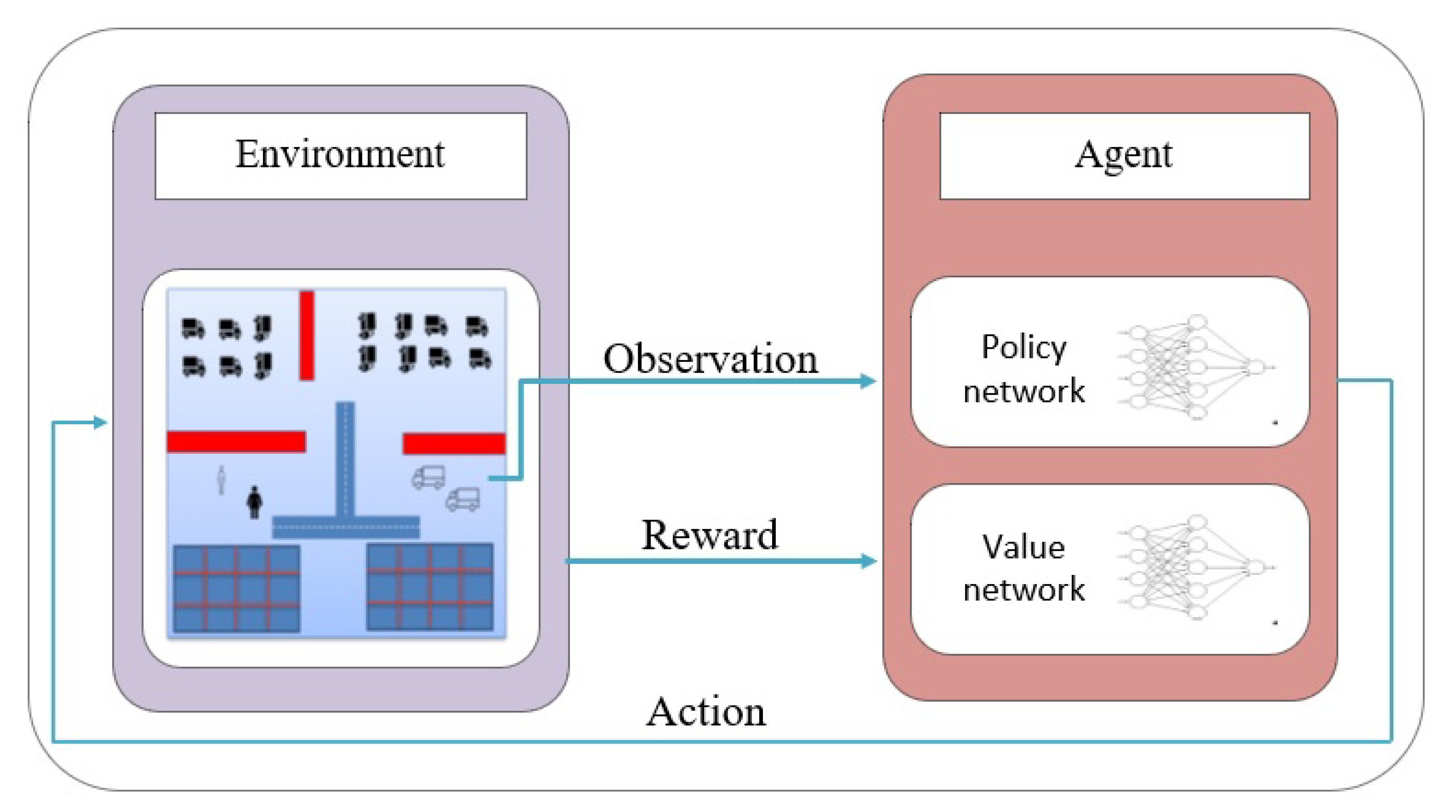
Unity3D was used to create the environment and simulate the training process. It enables realistic visuals and accurate physics, as well as low task complexity. The visualization was used to help evaluate the credibility of the system and as an illustration when communicating the solution to employees at Stena Line. Task complexity could be reduced through the task handling mechanism inside Unity3D. We made use also of the Unity ML-Agents [35] to train the agents since it contains a low-level Python interface that allows interacting with and manipulating the learning environment. In fact, the ML-Agents Toolkit contains five high-level components Figure 2, and herein, we explain the four components that we used and show their role in our application:
- Learning Environment: It contains the scene and all game characters. The Unity scene provides the environment in which agents observe, act, and learn. In our experiments, the same scene was used for both training and testing the trained agents. It represents the internal decks of the RORO where trailers are placed and the quay or wharf, which is a reinforced bank where trailers stand or line-up. It includes also linkspans, trailers, tug masters, and various dynamic and static objects. The internal decks can be of various sizes and may be on different floors.From a pure learning perspective, this environment contains two sub-components: Agent and Behavior. The Agentis attached to the Unity game object tug master and represents the learner. The Behavior can be thought of as a function that receives observations and rewards from the Agent and returns actions. There are three types of behaviors: learning, heuristic, or inference. A learning behavior is dynamic and not yet defined, but about to be trained. It is used to explore the environment and learn the optimal policy and presents the intermediate step before having the trained model and using it for inference. That is to say that the inference behavior is accomplished by the trained model, which is supposed to be optimal. This behavior is derived from the saved model file. A heuristic behavior is one that is explicitly coded and includes a set of rules; we used it to ensure that our code is correct and the agent is able to perform actions. Generally, the agents can have different behavior components or may share the same one.
- Python Low-Level API: It contains a low-level Python interface to interact with and manipulate a learning environment. It communicates with Unity through the Communicatorto control the Academyduring the training process. It is then an external component.
- External Communicator: It connects the Learning Environmentwith the Python Low-Level API.
- Python Trainers: This contains the implementation of proximal policy optimization for agent training. The use of PPO as a deep learning algorithm is explained in detail in Section 3.2. The implementation is built on top of the open-source library TensorFlow [36], Version 2.2. The Python Trainers interface with the Python Low-Level API from which it receives the set of agent observations and rewards and gives back the actions to be performed by the tug masters.
3.2. Algorithm
The agent should perform a set of tasks , where each is moving trucks from different initial positions to the target states under certain constraints such as static obstacles’ distribution, dynamic obstacles, lane-following, and truck size. We consider the task as being a tuple: . The goal of our policy based approach is to optimize a stochastic policy , which is parameterized by . In other words, the objective is to find a strategy that allows the agents to accomplish the tasks from various initial states with limited experiences. Given the state of the environment at time t for task T, the learning model of our agent predicts a distribution of actions according to the policy, from which an action at is sampled. Then, the agent interacts with the environment performing the sampled action and receives an immediate reward according to the reward function. Afterwards, it perceives next state . In an iterative way, the learning model needs to optimize the loss function that maps a trajectory followed by the policy from an initial state to a finite horizon H. The loss of a trajectory is nothing but negative cumulative reward .
The policy learning is shown in Algorithm 1. In each episode, we collect N trajectories under the policy . Afterwards, the gradient of the loss function is computed with regard to the parameter , and the latter is updated accordingly.
| Algorithm 1: Pseudocode for policy learning. |
 |
3.3. DRL Implementation Workflow
The first task is to develop a realistic and complex environment with goal-oriented scenarios. The environment includes ship, walls, walking humans, rolling cargo, lanes, and tug masters. The cargo is uniformly distributed in random positions inside an area representing the quay where cargo should be queued. The maximum linear velocity in the x and y axes is 5 m/s, and the maximum angular velocity in the z axis is 2 rad/s. The agents observe the changes in the environment and collect the data, then send them along with reward signals to the behavior component, which will decide the proper actions. Then, they execute those actions within their environment and receive rewards. This cycle is repeated continuously until the convergence of the solution. The behavior component controlling the agents is responsible for learning the optimal policy. The learning process was divided into episodes with a length of time steps where the agent must complete the task. A discrete time step, i.e., a state, is terminal if:
- The agents collide with a dynamic obstacle.
- The maximal number of steps in the episode is achieved.
- The agents place all cargo in the destinations, which means that all tasks are completed.
Data collection: the set of observations that the agent perceives about the environment. Observations can be numeric or visual. Numeric observations measure the attributes of the environment using sensors, and the visual inputs are images generated from the cameras attached to the agent and represent what the agent is seeing at that point in time. In our application, we use the ray perception sensors, which measure the distance to the surrounding objects. The inputs of the value/policy network are collected instantly by the agents and consist of their local state information. The agents navigate according to this local information, which represents the relative position of agents to surrounding obstacles using nine raycast sensors with between them. No global state data are received from the agents, such as absolute position or orientation in a coordinate reference. In addition, we feed to the input of the neural network other data like the attributes of the sensed cargo.
The agents share the same behavior component. This means that they will learn the same policy and share experience data during the training. If one of the agents discovers an area or tries some actions, then the others will learn from that automatically. This helps to speed up the training.
Action space: the set of actions the agent can take. Actions can either be continuous or discrete depending on the complexity of the environment and agent. In the simulation, the agent can move, rotate, pull, and release the cargo and select the destination where to release the dragged cargo.
Reward shaping: Reward shaping is one of the most important and delicate operations in RL. Since the agent is reward motivated and is going to learn how to act by trial experiences in the environment, simple and goal-oriented functions of rewards need to be defined.
According to this multi-task setting, we implement reward schemes to fulfil each task and achieve the second sub-goal since the task functions are relatively decoupled from each other and, in particular, the relationship between collision avoidance and path planning maneuvers and placement constraints. We train the agent with deep RL to obtain the skill of moving from different positions with various orientations to a target pose while considering the time and collision avoidance, as well as the constraints from both the agent and placement space. Thus, each constraint stated in the specifications should have its appropriate reward and/or penalty function. The reward can be immediate after each action or transition from state-to-state and measured as the cumulative reward at the end of the episode. In addition, the sparse reward function is used instead of continuous rewards since the relationship between the current state and goal is nonlinear.
- During the episode:
- −
- The task must be completed on time. Therefore, after each action, a negative reward is given to encourage the agent to finish the mission quickly. It equals such that is the maximum number of steps allowed for an episode.
- −
- If an object is transported to the right destination, a positive reward is given.
- After episode completion: If all tasks are finished, a positive reward is given .
- Static collision avoidance: Agents receive a negative reward (−1) if they collide with a static obstacle. Box colliders are used to detect the collisions with objects in Unity3D.
- Dynamic collision avoidance: There are two reward schemes: the episode must be terminated if a dynamic obstacle is hit, which means that the tug master fails to accomplish the mission; the second option is to assign a negative reward to the agent and let it finish the episode. A successful avoidance is rewarded as well. To enhance the safety and since dynamic obstacles are usually humans, the second choice is adopted.
- Lane-following: No map or explicit rules are provided to the agent. The agent relies solely on the reward system to navigate, which makes this task different from path following in which a series of waypoints to follow is given to the agent. The agent is rewarded for staying on the lane continuously, i.e., in each step, and since the agent often enters and leaves the lanes during the training, the rewards for lane-following have to be very small so that they do not influence the learning of the objective.
- −
- Entering the lane: positive reward .
- −
- Staying in the lane: positive reward .
- −
- Going out of the lane: negative reward ; should be larger than the entry reward to avoid zigzag behavior.
If we suppose that the lanes are obstacle-free, the accumulated reward is the sum of the obtained rewards during the episode. Otherwise, obstacle avoidance and lane-following are considered as competing objectives. Then, a coefficient is introduced to make a trade-off between them, as described by Equation (1), with and being the lane-following and obstacle avoidance rewards at time t, respectively.
Configuration parameters: The most important parameters are explained in the following lines, and the others are summarized in Table 1.
- Batch size: the number of training samples (observations) fed to the network in one iteration; its value is set to 1024.
- Number of epochs: Each epoch is one complete presentation of the dataset to be learned by a learning machine. After each epoch, the model weights are updated. Each epoch includes many iterations (data size divided by the batch size), and each iteration consists of one feed-forward and back-propagation of only one batch. Three epochs are generally sufficient to digest all the data features.
- Learning rate: controls the change amount made by adjusting the weights of the network with respect to the loss gradient, called also the step size. It can simply be defined as how much newly acquired information overrides the old. The learning rate is the most important hyperparameter to tune to achieve good performance in the problem, commonly denoted as beta.
- Epsilon decay: controls the decrease in the learning rate so that the exploration and exploitation are balanced throughout the learning. Exploration means that the agent searches over the whole space in the hope to find new states that potentially yield higher rewards in the future. On the other hand, exploitation means the agent’s tendency to exploit the promising states that return the highest reward based on existing knowledge. The value of epsilon decay is generally set around .
The parameter values exposed herein are the default values recommended for general tasks. For our specific task, optimal hyperparameters are obtained using tuning techniques. In fact, one of the big challenges of DRL is the selection of hyperparameter values. DRL methods include parameters not only for the deep learning model, which learns the policy, but also in the environment and the exploration strategy. The parameters related to the model design make it possible to construct a deep learning model capable of effectively learning latent features of the sampled observations; whereas a proper choice of parameters related to the training process allows the built model to speed up the learning and converge towards the objective.
The hyperparameter optimization problem (HPO) is a challenging task since the hyperparameters interact with each other and do not act independently, which makes the search space very huge. Different types of methods have been used to solve the HPO problem. Basic search methods sample the search space according to a very simple rule and without a guiding strategy, such as the grid search method and the random search method [37]. More advanced methods are sample based and use a policy to guide the sampling process and update the policy based on evaluating the new sample. The well-known algorithms of this category are Bayesian based optimizers [38] and population based techniques such as the genetic algorithm, which we opt to use in this paper [39]. The challenge here is to find a policy that finds the optimal configuration in a few iterations and avoids local optima. The last category includes HPO gradient based methods that perform the optimization by directly computing the partial derivative of the loss function on the validation set [40].
All the experiments were done using Unity3D Version 2018.4 and ML-Agents v.1.1.0 developed by Unity technologies, San Francisco, US. C# was used to create the environment and scripts controlling the agents, while Python was used to develop the learning techniques and train the agents. The external communicator of Unity allows the agent training using the Python code. The agents use the same brain, which means that their observations are sent to the same model to learn a shared policy. A machine with the microprocessor Intel i7 and a RAM size of 16G was used to run the implemented code.
4. Results and Discussion
4.1. Agent Learning Evaluation
The simulations were performed using a multiagent framework. Two agents, representing tug masters, collaborated to place the cargo in their appropriate locations. We analyzed the agent’s performance based on quantitative metrics, and Table 1 summarizes the most important parameters used in the simulation.
Four scenarios were considered. In the first scenario, the surface (100 m × 100 m) where the agents learned to move the rolling cargo was obstacle-free. The agents were not constrained to follow lanes, and the only requirement was to complete the task as quickly as possible. About 2.7 M steps of training were enough to converge, and then, the agents could complete all tasks in an average of 300 steps with a mean cumulative reward of for 7000 steps.
The second scenario consisted of lane-following and static obstacle avoidance (walls). About 3.6 M episodes were required to achieve the convergence where the success rate of avoiding static obstacles was and the average time needed to complete the task was 410 steps. The mean accumulated reward was , which decreased compared to the first scenario due to the increase of the path length caused mainly by the existence of obstacles. The third scenario included dynamic obstacles, i.e., pedestrians. The success rate of the agent to avoid those dynamic obstacles was about , and it learned to avoid static obstacles . In the fourth scenario, the agent learned all tasks.
Table 2 summarizes the overall training progress for different scenarios. Converge is the number of steps it took to converge. Reward is the mean cumulative reward, and reward std is the standard deviation. Length is the episode length after convergence. To compare the learning behavior, the mean cumulative reward of 7000 steps was computed for all agents. As expected, it consistently increased over time during the training phase (Figure 3). The fluctuation of the curve reflects the successive unsuccessful episodes. After the convergence, the curve should be stationary and fluctuations reduced. The standard deviation of the cumulative episode reward lied in the interval , which appeals to the implementation of the stabilization technique as mentioned in Section 5. Three-hundred to 450 steps were required for each agent to accomplish the mission collaboratively.
The lane-following was qualitatively evaluated. The agents followed the lanes almost perfectly, but for some sequences, they still tended to choose the shortest path, so that they saved time and got a greater reward.
Figure 4 shows also how much reward the agent predicted to receive in the short term through the value estimate metric. It is the mean value estimate for all states visited by the agent during the episode. It increased during the successful training sessions and increased throughout the learning. After some time, the mean value estimate became almost proportional with to the cumulative reward increased. This means that the agent was accurately learning to predict the rewards. The same figure depicts the linear evolution of the learning rate by a decay of .
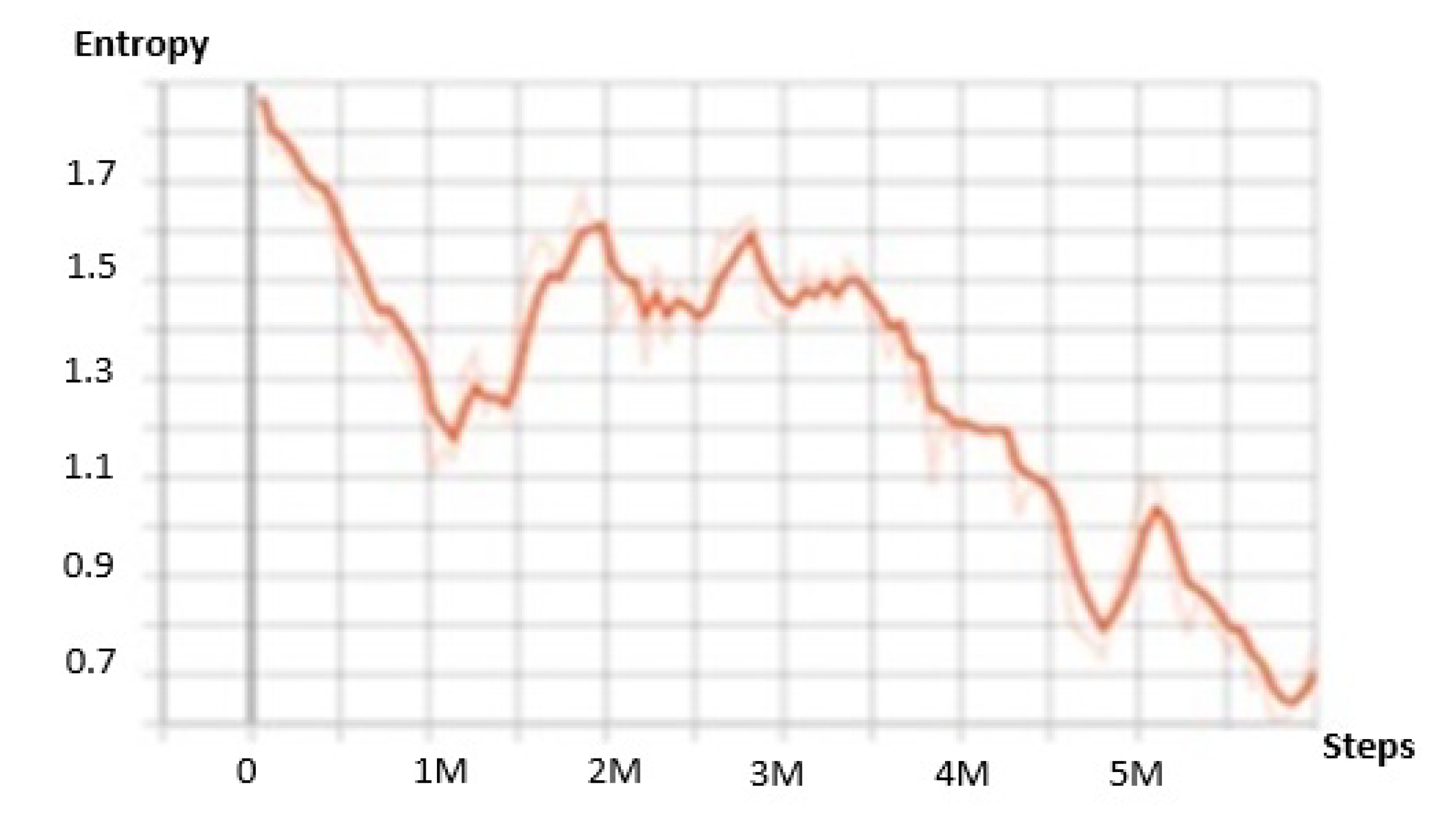
To evaluate the learning progress of the agents, various metrics were used. In Figure 5, the entropy measures the randomness and uncertainty of the model decisions. It reflects the expected information content and quantifies the surprise in the action outcome. As shown in the figure, it steadily decreased during a successful training episode and consistently decreased during the entire training process. The increase in the entropy, for instance between the steps 1.1 Mand 2 M, shows that the agents were exploring new regions of the state space for which they did not have much information.
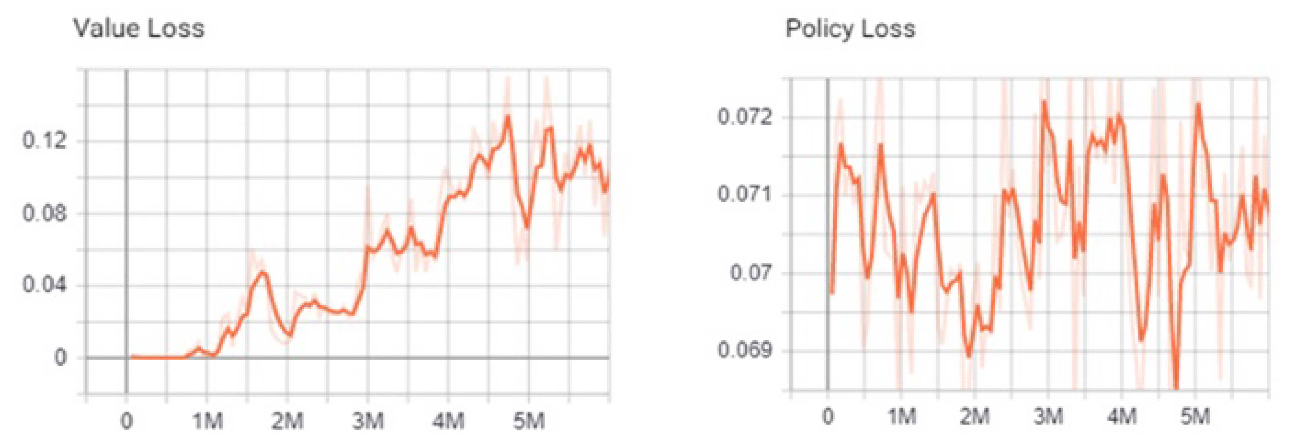
To evaluate how the state space was learned by the agents, the value loss metric was used. It computes the mean loss of the value function update for each iteration, subsequently reflecting the ability of the model to predict the value of each state. As shown in Figure 6, it increased during the training and then decreased once the learning converged. This shows that the agents learned the state space accurately. On the other hand, the policy loss was the mean magnitude of the policy loss function. It reflects the way in which the policy, i.e., the strategy of action decision, evolved. The results show that, as expected, it oscillated during training, and its magnitude decreased for each successful session when the agents chose the best action sequences.
4.2. Incremental Learning
In the case of complex environments, the agent may take a long time to figure out the desired tasks. By simplifying the environment at the beginning of training, we allowed the agent to quickly update the random policy to a more meaningful one that was successively improved as the environment gradually increased in complexity. We proceeded in an incremental way as follows: we trained the agents in a simplified environment, then we used the trained agents in the next stage with more complex tasks, and so forth. There was no need to retrain them from scratch. Table 3 depicts the different stages of the incremental learning. Converge is the number of steps required for convergence; Reward is the mean cumulative reward; and Length is the episode length after convergence. After training the agent in the basic scenario without obstacles and lanes, it took only 1.5 M to teach the agent to follow lanes and avoid static obstacles instead of spending 3.6 M steps to learn the tasks from scratch. The same was for learning dynamic obstacle avoidance, which required only an extra 1.9 M steps. The same experience was performed for five iterations and showed that the agent was learning a sub-optimal policy with a reward average of 13 and never exceeded .
4.3. Hyperparameter Tuning
The final experiment aimed to improve the results obtained using default hyperparameters. The genetic algorithm (GA) was used as an optimizer over the hyperparameter search spaces to find the optimal structure of the model, as well as to tune the hyperparameters of the model training process. The optimizer was run for 100 generations with a population of size 20 in a parallel computation scheme such that the maximum number of iterations was one million steps. Each individual presented a single combination of the hyperparameters. The fitness function was evaluated once the stop condition was met for all individuals, and it equaled the mean of accumulated rewards for the last 100 episodes. Table 4 shows the search space considered for the model design hyperparameters and the obtained optimal values. The discrete sets are denoted by parentheses, and continuous intervals are denoted with brackets and sampled uniformly by the GA. The optimal architecture of the deep learning model that learned the policy and the advantage function consisted of three hidden layers having each 256 units.
The optimal parameters for the training process are listed in Table 5. The use of this value combination sped up the learning process and increased the mean cumulative reward. A full simulation for the fourth scenario shows that the agents achieved a mean cumulative reward of in 4.6 M steps.
To show the importance of hyperparameter tuning, Figure 7 illustrates the learning progress of the agents for different hyperparameter values in the fourth scenario. It is clear that choosing the values of configuration degraded the performance of the agents, and never learned the tasks. In fact, we noticed through the visualization that they could not explore the environment and were stuck in a sub-region of the space. Using the value combinations and allowed the agents to learn a suboptimal policy because they did not complete all tasks in an optimized time and their risk of hitting obstacles was high.
4.4. Discussion
Looking back at the research questions formulated in the Introduction, we can affirm that the agents are able to learn good strategies and fulfil the expected tasks. Regarding the first research question, we can say that using appropriate model hyperparameters, we can converge to a solution where the agents learn how to accomplish their tasks. The convergence also ensures some kind of stability and allows the agents to exploit their knowledge instead of infinitely exploring the environment or choosing random actions. However, the reward standard deviation reflects the trajectories’ variation and also the imperfection of learning stability. Looking at the second research question, we can see that the policy learned is sub-optimal in the incremental learning approach, but it is near-optimal otherwise. Regarding the third research question, it is evident that the tuning of hyperparameters improved the quality of the achieved solution.
The obtained results are very promising and encourage resolving more advanced logistics constraints using reinforcement learning. Our study was limited to collision avoidance, lane-following, and cargo moving. In addition, only one cargo feature, which is the size, is used as the constraint to place the cargo in its appropriate destination. Thus, the formulation of the multi-objective stowage problem including all the logistics constraints is one of the first priorities. The aim will be mainly the optimization of the deck utilization ratio on board the ship with respect to specific constraints such as customer priorities, placing vehicles that belong to the same customer close to each other, ship weight balance, etc. Another perspective of this study that currently presents a challenge to the proposed autonomous system is the stability. In fact, the reward standard deviation lies between in the first scenario without obstacles and for the fourth scenario. Lyapunov function based approaches [41] can be used on the value function to ensure that the RL process is bounded by a maximum reward region. In addition, collaboration among the agents can be further enhanced. In this paper, a parameter-sharing strategy is used to ensure the collaboration and implicit knowledge sharing, which means that the policy parameters are shared among the agents. However, cooperation is still limited without explicitly sharing the information.
5. Concluding Remarks
In this paper, deep reinforcement learning is used to perform recurrent and important logistics operations in maritime transport, namely rolling cargo handling. The agents, representing the tug masters, successfully learn to move all cargo from the initial positions to the appropriate destinations. Avoiding static and dynamic obstacles is included in the objective function of the agents. The agents learn to avoid static obstacles with a success rate and avoid dynamic obstacles with a success rate. We use hyperparameter tuning to improve the results, and we show the great impact that deep learning model hyperparameters have on the solution convergence, policy learning, and advantage function. In the tuned model, the agents need 4.6 M steps to converge towards the optimal policy and achieve of the maximum value of the mean cumulative reward. Finally, incremental learning has the advantage of saving training time and building a complex environment incrementally, but it risks falling into a local optimal trap.
The proposed approach shows a potential to be extended to real-world problems where full automation of the loading/unloading operations would be feasible. The impact would be for both environmental sustainability and potential increase in revenue. The work should also be of interest to manufacturers of systems and vehicles used in these settings. However, as pointed out, this is an initial study and as such the main focus has been on studying the feasibility to apply the algorithms presented in the work and to see if they can solve a simplified problem of unloading and loading of cargo.
We see several possible extensions of the proposed solution as directions for future work. As the end goal is to implement it in physical tug masters loading and unloading ROROs, incorporating more realistic constraints is one extension that we will pursue. This includes making the agents operate with realistic tug master constraints, like having to reverse in order to attach a trailer, having to drag the trailer, and being realistically affected by dragging a heavy trailer regarding, e.g., acceleration, breaking, turning, etc. This also includes making the interior of the ROROs more realistic, with multiple decks, narrow passages, etc. Another aspect that might need consideration is load balancing on deck, in order to optimize stability and minimize fuel consumption. Several of the mentioned improvements will affect the RL environment, but will also need reshaping of the reward function. Optimizing the reward function to ensure that the agents learn to avoid dynamic obstacles perfectly is another important thing to address in future work.
Author Contributions
Conceptualization, R.O., T.L., E.A. and L.C.; Methodology, R.O., T.L., E.A. and L.C.; Software, R.O..; Validation, R.O., T.L., E.A. and L.C.; Formal Analysis, R.O., T.L., E.A. and L.C.; Investigation, R.O., T.L., E.A. and L.C.; Resources, R.O., T.L., E.A. and L.C; Data Curation, R.O.; Writing— Original Draft Preparation, R.O., T.L., E.A. and L.C; Writing—Review & Editing, R.O., T.L., E.A. and L.C; Visualization, R.O; Supervision, R.O., T.L., E.A. and L.C; Project Administration, T.L. and E.A.; Funding Acquisition, T.L., E.A. and L.C. All authors read and agreed to the published version of the manuscript.
Funding
This research was funded by Swedish Knowledge Foundation Grant Number DATAKIND 20190194.
Institutional Review Board Statement
Not applicable.
Informed Consent Statement
Not applicable.
Data Availability Statement
Code repository: github.com/Rachidovij/RL-CargoManagement (accessed on 7 February 2021).
Acknowledgments
This work was supported by the Swedish Knowledge Foundation (DATAKIND 20190194).
Conflicts of Interest
The authors declare no conflict of interest.
Abbreviations
The following abbreviations are used in this manuscript:
| AI | Artificial intelligence |
| ML | Machine learning |
| RL | Reinforcement learning |
| DRL | Deep RL |
| RORO | Roll-on/roll-off ships |
| TRPO | Trust region policy optimization |
| PPO | Proximal policy optimization |
| DNN | Depp neural network |
| DL | Deep learning |
| HPO | Hyperparameter optimization |
| GA | Genetic algorithm |
References
- Zarzuelo, I.D.L.P.; Soeane, M.J.F.; Bermúdez, B.L. Industry 4.0 In the Port and Maritime Industry: A Literature Review. J. Ind. Inf. Integr. 2020, 100173. [Google Scholar] [CrossRef]
- Orive, A.C.; Santiago, J.I.P.; Corral, M.M.E.I.; González-Cancelas, N. Strategic Analysis of the Automation of Container Port Terminals through BOT (Business Observation Tool). Logistics 2020, 4, 3. [Google Scholar] [CrossRef] [Green Version]
- Hirashima, Y.; Takeda, K.; Harada, S.; Deng, M.; Inoue, A. A Q-Learning for group based plan of container transfer scheduling. JSME Int. J. Ser. Mech. Syst. Mach. Elem. Manuf. 2006, 49, 473–479. [Google Scholar] [CrossRef] [Green Version]
- Priyanta, I.F.; Golatowski, F.; Schulz, T.; Timmermann, D. Evaluation of LoRa Technology for Vehicle and Asset Tracking in Smart Harbors. In Proceedings of the IECON 2019—45th Annual Conference of the IEEE Industrial Electronics Society, Lisbon, Portugal, 14–19 October 2019; Volume 1, pp. 4221–4228. [Google Scholar]
- Yau, K.A.; Peng, S.; Qadir, J.; Low, Y.; Ling, M.H. Towards Smart Port Infrastructures: Enhancing Port Activities Using Information and Communications Technology. IEEE Access 2020, 8, 83387–83404. [Google Scholar] [CrossRef]
- Munim, Z.H.; Dushenko, M.; Jimenez, V.J.; Shakil, M.H.; Imset, M. Big data and artificial intelligence in the maritime industry: A bibliometric review and future research directions. Marit. Policy Manag. 2020, 47, 577–597. [Google Scholar] [CrossRef]
- Barua, L.; Zou, B.; Zhou, Y. Machine learning for international freight transportation management: A comprehensive review. Res. Transp. Bus. Manag. 2020, 34, 100453. [Google Scholar] [CrossRef]
- Mnih, V.; Kavukcuoglu, K.; Silver, D.; Graves, A.; Antonoglou, I.; Wierstra, D.; Riedmiller, M. Playing atari with deep reinforcement learning. arXiv 2013, arXiv:1312.5602. [Google Scholar]
- Silver, D.; Schrittwieser, J.; Simonyan, K.; Antonoglou, I.; Huang, A.; Guez, A.; Hubert, T.; Baker, L.; Lai, M.; Bolton, A.; et al. Mastering the game of go without human knowledge. Nature 2017, 550, 354–359. [Google Scholar] [CrossRef] [PubMed]
- Andrychowicz, O.M.; Baker, B.; Chociej, M.; Jozefowicz, R.; McGrew, B.; Pachocki, J.; Petron, A.; Plappert, M.; Powell, G.; Ray, A.; et al. Learning dexterous in-hand manipulation. Int. J. Robot. Res. 2020, 39, 3–20. [Google Scholar] [CrossRef] [Green Version]
- Shen, Y.; Zhao, N.; Xia, M.; Du, X. A Deep Q-Learning Network for Ship Stowage Planning Problem. Pol. Marit. Res. 2017, 24, 102–109. [Google Scholar] [CrossRef] [Green Version]
- Lee, C.; Lee, M.; Shin, J. Lashing Force Prediction Model with Multimodal Deep Learning and AutoML for Stowage Planning Automation in Containerships. Logistics 2020, 5, 1. [Google Scholar] [CrossRef]
- Zhang, C.; Guan, H.; Yuan, Y.; Chen, W.; Wu, T. Machine learning-driven algorithms for the container relocation problem. Transp. Res. Part B Methodol. 2020, 139, 102–131. [Google Scholar] [CrossRef]
- Hottung, A.; Tanaka, S.; Tierney, K. Deep learning assisted heuristic tree search for the container pre-marshalling problem. Comput. Oper. Res. 2020, 113, 104781. [Google Scholar] [CrossRef]
- Price, L.C.; Chen, J.; Cho, Y.K. Dynamic Crane Workspace Update for Collision Avoidance During Blind Lift Operations. In Proceedings of the 18th International Conference on Computing in Civil and Building Engineering, Sao Paulo, Brazil, 18–20 August 2020; Toledo Santos, E., Scheer, S., Eds.; Springer: Cham, Switzerland, 2021; pp. 959–970. [Google Scholar] [CrossRef]
- Atak, Ü.; Kaya, T.; Arslanoğlu, Y. Container Terminal Workload Modeling Using Machine Learning Techniques. In Intelligent and Fuzzy Techniques: Smart and Innovative Solutions; Kahraman, C., Cevik Onar, S., Oztaysi, B., Sari, I.U., Cebi, S., Tolga, A.C., Eds.; Springer: Cham, Switzerland, 2021; pp. 1149–1155. [Google Scholar] [CrossRef]
- M’hand, M.A.; Boulmakoul, A.; Badir, H.; Lbath, A. A scalable real-time tracking and monitoring architecture for logistics and transport in RoRo terminals. Procedia Comput. Sci. 2019, 151, 218–225. [Google Scholar] [CrossRef]
- M’hand, M.A.; Boulmakoul, A.; Badir, H. On the exploitation of Process mining and Complex event processing in maritime logistics: RoRo terminals. In Proceedings of the International Conference on Innovation and New Trends in Information Systems, Marrakech, Morocco, 2–3 May 2018. [Google Scholar]
- You, K.; Yu, M.; Yu, Q. Research and Application on Design of Underground Container Logistics System Based on Autonomous Container Truck. IOP Conf. Ser. Earth Environ. Sci. 2019, 330, 022054. [Google Scholar] [CrossRef]
- Øvstebø, B.O.; Hvattum, L.M.; Fagerholt, K. Optimization of stowage plans for RoRo ships. Comput. Oper. Res. 2011, 38, 1425–1434. [Google Scholar] [CrossRef]
- Puisa, R. Optimal stowage on Ro-Ro decks for efficiency and safety. J. Mar. Eng. Technol. 2018, 1–17. [Google Scholar] [CrossRef] [Green Version]
- Hansen, J.R.; Hukkelberg, I.; Fagerholt, K.; Stålhane, M.; Rakke, J.G. 2D-Packing with an Application to Stowage in Roll-On Roll-Off Liner Shipping. In Computational Logistics; Paias, A., Ruthmair, M., Voß, S., Eds.; Springer: Cham, Switzerland, 2016; pp. 35–49. [Google Scholar]
- Verma, R.; Saikia, S.; Khadilkar, H.; Agarwal, P.; Shroff, G.; Srinivasan, A. A Reinforcement Learning Framework for Container Selection and Ship Load Sequencing in Ports. In Proceedings of the 18th International Conference on Autonomous Agents and MultiAgent Systems (AAMAS ’19), Montréal, QC, Canada, 13–17 May 2019; Elkind, E., Manuela Veloso, N.A., Taylor, M.E., Eds.; International Foundation for Autonomous Agents and Multiagent Systems: Istanbul, Turkey, 2019; pp. 2250–2252. [Google Scholar]
- Fotuhi, F.; Huynh, N.; Vidal, J.M.; Xie, Y. Modeling yard crane operators as reinforcement learning agents. Res. Transp. Econ. 2013, 42, 3–12. [Google Scholar] [CrossRef]
- Hirashima, Y. An intelligent marshaling plan based on multi-positional desired layout in container yard terminals. In Proceedings of the 4th International Conference on Informatics in Control, Automation and Robotics, Angers, France, 9–12 May 2007; Zaytoon, J., Ferrier, J.L., Cetto, J.A., Filipe, J., Eds.; 2007; pp. 234–239. [Google Scholar]
- Jia, B.; Rytter, N.G.M.; Reinhardt, L.B.; Haulot, G.; Billesø, M.B. Estimating Discharge Time of Cargo Units—A Case of Ro-Ro Shipping. In Computational Logistics; Paternina-Arboleda, C., Voß, S., Eds.; Springer: Cham, Switzerland, 2019; pp. 122–135. [Google Scholar] [CrossRef]
- Tang, G.; Guo, Z.; Yu, X.; Song, X.; Wang, W.; Zhang, Y. Simulation and Modelling of Roll-on/roll-off Terminal Operation. In Proceedings of the 2015 International Conference on Electrical, Automation and Mechanical Engineering, Phuket, Thailand, 26–27 July 2015; Atlantis Press: Amsterdam, The Netherlands, 2015. [Google Scholar] [CrossRef] [Green Version]
- Sutton, R.S.; Barto, A.G. Reinforcement Learning: An Introduction; MIT Press: Cambridge, MA, USA, 2018. [Google Scholar]
- Schulman, J.; Moritz, P.; Levine, S.; Jordan, M.; Abbeel, P. High-Dimensional Continuous Control Using Generalized Advantage Estimation. arXiv 2015, arXiv:1506.02438. [Google Scholar]
- Schulman, J.; Levine, S.; Abbeel, P.; Jordan, M.; Moritz, P. Trust region policy optimization. In Proceedings of the International Conference on Machine Learning, Lille, France, 7–9 July 2015; pp. 1889–1897. [Google Scholar]
- Schulman, J.; Wolski, F.; Dhariwal, P.; Radford, A.; Klimov, O. Proximal policy optimization algorithms. arXiv 2017, arXiv:1707.06347. [Google Scholar]
- Dong, H.; Ding, Z.; Zhang, S. (Eds.) Deep Reinforcement Learning; Springer: Singapore, 2020. [Google Scholar] [CrossRef]
- Watkins, C.J.C.H.; Dayan, P. Q-learning. Mach. Learn. 1992, 8, 279–292. [Google Scholar] [CrossRef]
- Mnih, V.; Kavukcuoglu, K.; Silver, D.; Rusu, A.A.; Veness, J.; Bellemare, M.G.; Graves, A.; Riedmiller, M.; Fidjeland, A.K.; Ostrovski, G.; et al. Human-level control through deep reinforcement learning. Nature 2015, 518, 529–533. [Google Scholar] [CrossRef]
- Juliani, A.; Berges, V.P.; Teng, E.; Cohen, A.; Harper, J.; Elion, C.; Goy, C.; Gao, Y.; Henry, H.; Mattar, M.; et al. Unity: A General Platform for Intelligent Agents. arXiv 2018, arXiv:abs/1809.02627. [Google Scholar]
- Abadi, M.; Barham, P.; Chen, J.; Chen, Z.; Davis, A.; Dean, J.; Devin, M.; Ghemawat, S.; Irving, G.; Isard, M.; et al. TensorFlow: A system for large-scale machine learning. In Proceedings of the 12th USENIX Symposium on Operating Systems Design and Implementation (OSDI 16), San Diego, CA, USA, 2–4 November 2016; pp. 265–283. [Google Scholar]
- Florea, A.C.; Andonie, R. Weighted Random Search for Hyperparameter Optimization. arXiv 2020, arXiv:2004.01628. [Google Scholar] [CrossRef]
- Sui, G.; Yu, Y. Bayesian Contextual Bandits for Hyper Parameter Optimization. IEEE Access 2020, 8, 42971–42979. [Google Scholar] [CrossRef]
- Kim, J.; Cho, S. Evolutionary Optimization of Hyperparameters in Deep Learning Models. In Proceedings of the 2019 IEEE Congress on Evolutionary Computation (CEC), Wellington, New Zealand, 10–13 June 2019; pp. 831–837. [Google Scholar]
- Bakhteev, O.Y.; Strijov, V.V. Comprehensive analysis of gradient based hyperparameter optimization algorithms. Ann. Oper. Res. 2019, 289, 51–65. [Google Scholar] [CrossRef]
- Lyapunov, A.M. The general problem of the stability of motion. Int. J. Control 1992, 55, 531–534. [Google Scholar] [CrossRef]
Figure 1.
General structure of the navigation system explored in this study.

Figure 2.
ML-Agents architecture [35].
Figure 2.
ML-Agents architecture [35].

Figure 3.
Evolution of learning parameters during training (Scenario 4).

Figure 4.
Learning progress during training in the fourth scenario.

Figure 5.
Evolution of the entropy during the training (scenario 4).

Figure 6.
Evolution of losses during the training (Scenario 4).

Figure 7.
Agent learning progress for different hyperparameter configurations. Table 6 shows the corresponding combination values.
Figure 7.
Agent learning progress for different hyperparameter configurations. Table 6 shows the corresponding combination values.


Table 1.
Parameters used in the simulation and their values.
| Parameter | Value |
|---|---|
| Number of layers | 2 |
| Buffer size | 2048 |
| 0.95 | |
| Gamma | 0.99 |
| Learning rate schedule | linear |
| Memory size | 256 |
| Data normalization | false |
| Time horizon | 64 |
| Sequence length | 64 |
| Use recurrent | True |
| Summary frequency | 60,000 |
| Visualization encode type | simple |
| Maximum steps | |
| Number of hidden units in DNN | 128 |
Table 2.
Agent training performance for different scenarios.
| Scenario | Converge | Reward | Reward std | Length |
|---|---|---|---|---|
| Without obstacles and lanes | 2.7 M | 16.4 | 1.83 | 300 |
| Lane-following and static obstacles | 3.6 M | 15.7 | 2.13 | 410 |
| Static and dynamic obstacles | 3.4 M | 15 | 2.93 | 400 |
| Lane-following and obstacle avoidance | 5.7 M | 13.9 | 3.2 | 450 |
Table 3.
Mean of the accumulated rewards and convergence speed for different scenarios.
| Environment Complexity | Converge | Reward | Length |
|---|---|---|---|
| Without obstacles and lanes | 2.7 M | 16.4 | 300 |
| Lane-following and static obstacles | 4.2 M | 15.1 | 430 |
| Lane-following and obstacle avoidance | 6.1 M | 13 | 530 |
Table 4.
Search spaces and optimal values of the model structure hyperparameters.
| Search Space | Optimal Values | |
|---|---|---|
| # of hidden layers | (2, 3, 4, 5) | 3 |
| # of units in the hidden layer | (128, 160, 256, 512) | 256 |
| dropout | [0.01, 0.3] | 0.22 |
Table 5.
Learning parameters explored.
| Search Space | Optimal Values | |
|---|---|---|
| Learning rate | [] | |
| Epsilon decay | [0.1, 0.3] | 0.18 |
| Batch size | (512, 1024, 1536, 2048) | 512 |
| [0.9, 0.99] | 0.9 | |
| Maximum episode length | [500, 800] | 564 |
Table 6.
Hyperparameter configurations used in the experiment of Figure 7.
Table 6.
Hyperparameter configurations used in the experiment of Figure 7.
| C1 | C2 | C3 | C4 | |
|---|---|---|---|---|
| Learning rate | ||||
| Epsilon decay | 0.18 | 0.26 | 0.24 | 0.28 |
| Batch size | 512 | 512 | 256 | 256 |
| 0.9 | 0.95 | 0.96 | 0.96 | |
| Maximum episode length | 564 | 592 | 630 | 510 |
| # of hidden layers | 3 | 3 | 2 | 2 |
| # of units in the hidden layer | 256 | 128 | 128 | 128 |
| Dropout | 0.22 | 0.06 | 0.15 | 0.28 |
Publisher’s Note: MDPI stays neutral with regard to jurisdictional claims in published maps and institutional affiliations. |
© 2021 by the authors. Licensee MDPI, Basel, Switzerland. This article is an open access article distributed under the terms and conditions of the Creative Commons Attribution (CC BY) license (http://creativecommons.org/licenses/by/4.0/).
Share and Cite
MDPI and ACS Style
Oucheikh, R.; Löfström, T.; Ahlberg, E.; Carlsson, L. Rolling Cargo Management Using a Deep Reinforcement Learning Approach. Logistics 2021, 5, 10. https://0-doi-org.brum.beds.ac.uk/10.3390/logistics5010010
AMA Style
Oucheikh R, Löfström T, Ahlberg E, Carlsson L. Rolling Cargo Management Using a Deep Reinforcement Learning Approach. Logistics. 2021; 5(1):10. https://0-doi-org.brum.beds.ac.uk/10.3390/logistics5010010
Chicago/Turabian StyleOucheikh, Rachid, Tuwe Löfström, Ernst Ahlberg, and Lars Carlsson. 2021. "Rolling Cargo Management Using a Deep Reinforcement Learning Approach" Logistics 5, no. 1: 10. https://0-doi-org.brum.beds.ac.uk/10.3390/logistics5010010