Closed-Loop Supply Chain Network Design under Uncertainties Using Fuzzy Decision Making

Abstract

The importance of considering forward and backward flows simultaneously in supply chain networks spurs an interest to develop closed-loop supply chain networks (CLSCN). Due to the expanded scope in the supply chain, designing CLSCN often faces significant uncertainties. This paper proposes a fuzzy multi-objective mixed-integer linear programming model to deal with uncertain parameters in CLSCN. The two objective functions are minimization of overall system costs and minimization of negative environmental impact. Negative environmental impacts are measured and quantified through CO₂ equivalent emission. Uncertainties include demand, return, scrap rate, manufacturing cost and negative environmental factors. The original formulation with uncertain parameters is firstly converted into a crisp model and then an aggregation function is applied to combine the objective functions. Numerical experiments have been carried out to demonstrate the effectiveness of the proposed model formulation and solution approach. Sensitivity analyses on degree of feasibility, the weighing of objective functions and coefficient of compensation have been conducted. This model can be applied to a variety of real-world situations, such as in the manufacturing production processes.

1. Introduction

The increasing need for re manufacturing, the growing market competition, and the concern on negative environmental impacts have spurred significant interest in closed-loop supply chain network (CLSCN) adoption in manufacturing industry. In contrast to designing the forward and reverse material flows separately, the integrated system can achieve global optimally considering both flows in the supply chain. As pointed out by Klibi et al., the complex and dynamic nature of CLSCN creates a lot of uncertainties in the supply chain system and dramatically influences the overall performance of the logistics [1]. The design of a supply chain network often involves long-term strategic decisions which have sustaining impact in business operations. Pishvaee et al. stated that opening/closing or upgrading a facility are capital intensive and time-consuming, and hence making any changes to those decisions in real time is often impossible [2]. Therefore, it is essential to incorporate uncertainties into the design of CLSCN such that the decisions in the supply chain network configuration are efficient and robust.

In this paper, we propose a mathematical model for a single-product, multi-period and capacitated CLSCN. The tactical decisions include determining flows among the facilities while strategic decisions involve facility location selection. The major contributions can be summarized as follows:

• We proposed a novel multi-objective CLSCN model to minimize overall system costs and negative environmental impact. To the best of authors’ knowledge, fuzzy programming has not been applied to CLSCN problems with system cost and environmental impact objectives.
• We found most related studies in the literature only considered 1 or 2 uncertain parameters. In this paper, we studied multiple uncertain parameters such as demand, return, scrap rate, processing costs and environmental impact.
• A comprehensive parameter sensitivity analysis of the fuzzy model is conducted.

The remainder of this paper is organized as follows: The literature review is discussed in Section 2. The problem statement and model formulation are defined in Section 3. The equivalent crisp model as well as solution approach are presented in Section 4. The computational experiments and sensitivity analyses are included in Section 5, and managerial insights are derived. Finally, Section 6 concludes the paper with major findings and points out future research directions.

2. Literature Review

There has been extensive study in this field. Scenario-based stochastic programming, robust optimization, and fuzzy programming approaches have been widely applied in CLSCN to deal with uncertainties. Scenario-based stochastic programming is a powerful approach when probabilistic distribution information for the uncertain parameter is available. A few recent studies estimate the probabilistic distributions for the uncertain parameters and then apply scenario-based stochastic programming which samples scenarios from the probabilistic distributions followed by scenario reduction techniques [3,4,5]. However, this approach has limitations [6,7]. First, in many real-world applications the decision maker may not have enough historical data, thus, estimating the accurate probabilistic distribution is impossible. For instance, estimating probabilistic distribution of demand of new product can be challenging. Second, an accurate approximation of probabilistic distribution may require a large amount of scenarios which increase the computational complexity. On the other hand, if scenario sample size is restricted for computational reasons, then the range of future realizations under which decisions are determined and evaluated is limited.

To address these limitations, robust optimization has been introduced as an alternative approach to deal with uncertainty. Robust optimization handles uncertainties by solving robust counterpart over predetermined uncertainty sets [8]. The robust counterpart is a worst-case formulation of the original problem in which worst-case is measured over all possible values that uncertain parameters may take in given convex sets. The main advantage of robust optimization in contrast to scenario-based stochastic programming is that only rough historical data is required to derive the uncertainty sets [9]. Studies that apply robust optimization to CLSCN can be found in the following literatures [2,10]. On top of that, there are papers that apply multiple methods, simultaneously. Hybrid robust and stochastic programming approach for multiple uncertainties have been studied in the following literatures [11,12]. However, the main limitations on robust optimization are: First, only a few uncertain parameters were considered in robust optimization for CLSCN mainly due to reformulation as well as computational complexity [2,10,13]. As stated by Prajogo and Olhager, supply chain network design often involves decisions from multiple stakeholders and significant amount of uncertainties [14]. Second, robust optimization assumes all uncertain coefficients belong to a predefined symmetric interval centered at the nominal value. This may not be true for some real-world applications in which uncertainties have highly skewed distributions [15]. Third, robust optimization assumes uncertainty to affect only the constraint coefficients. It should be noted that a problem with uncertainties in the objective functions or right hand side of constraints requires reformulation and thus increase computational complexity.

As an alternative, the main advantages of fuzzy programming are: First, this approach provides a framework to handle multiple uncertainties at the same time without increasing model complexity [16]. Those uncertainties can affect not only left hand side of constraints but also right hand side of constraints as well as objective function. Second, this approach does not require complete information about uncertainty. Uncertainties in the fuzzy programming are dealt with triangular or trapezoidal membership function in which only rough data is required to determine the most pessimistic value, the most possible value and the most optimistic value. Pishvaee and Torabi introduced a fuzzy mathematical programming model for CLSCN with two objective functions: minimization of total costs and minimization of total delivery tardiness [17]. Zarandi et al. considered uncertainties in the decision maker’s aspiration levels as the objectives are imprecise. There are four different objective functions in the paper: first two objective functions aim to minimize the overall costs and the last two objective functions focus on the maximization of total service level [18]. Jindal and Sangwan introduced a fuzzy mixed integer linear programming model for CLSCN with a single objective function which maximizes the overall profit [19]. Kumar and Kumar compared a traditional supply chain network system with a closed-loop supply chain network system and made the following claim: The traditional supply chain seeks to reduce the cost and improve the efficiency while CLSCN aims to lower the consumption of resources and decrease the emissions of pollutants so as to maximize the economic benefits [20]. Amin and Zhang emphasized the importance of considering environmental impact in CLSCN because environmental protection is included in the both internal and external management [21]. Literature also contains a review of the current research in CLSCN. Ehsan and Simme discuss many papers on CLSCs and game theory. They summarise that research has focused on duel channel collection and duel channel selling methods prioritizing the role of manufactures [22]. In addition to that, studies focusing on investigating factors contributing to CLSCN have also been published [23].

3. Problem Definition and Formulation

3.1. Problem Statement

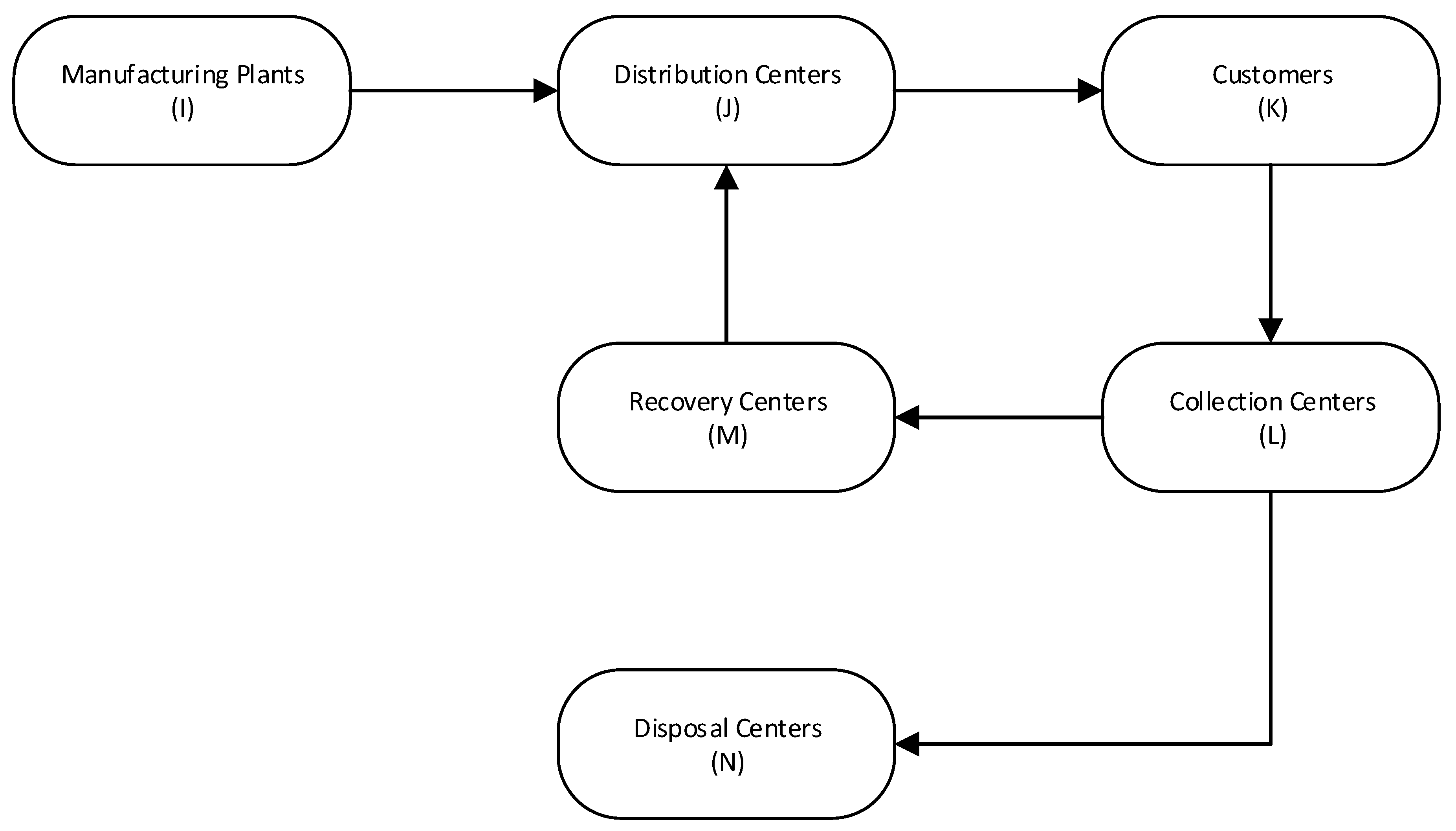
The network design problem studied in this paper is a single product, multi-period and capacitated CLSCN which includes manufacturing plants, distribution, collection, recovery and disposal centers. The configuration is explained in Figure 1 created by the authors. Given the customer demands, the goal is to find the optimal facility locations as well as materials flows such that overall system costs and negative environmental impacts are minimized. With concern over global climate increases, regulations on carbon emissions have been developed by government in multiple countries. For example, China has announced that Ministry of Finance would levy taxes on carbon emissions. In addition, European Union initialized a carbon emission trading scheme (EU ETS) for companies with the goal of reducing carbon emission [24]. Motivated by the effect of carbon emission, the negative environmental impacts are measured and quantified by CO₂ equivalent emission. We assume that facilities that have less negative environmental impact will require additional capital investment, therefore, negative environmental impacts are inversely proportional to capital investment. Haddadsisakht and Ryan emphasized the importance of studying carbon emission in the CLSCN [25].

This supply chain system consists of both forward and backward flows. In the forward network, manufacturing plants produce and transport products to distribution centers and then to customers. In the backward network, defective/used products are collected from customers and shipped to collection centers. After a quality examination process, returned products are classified into two different categories depending on their conditions. The recoverable and scrapped items are sent to recovery and disposal centers, respectively. After appropriate processing, recovered items are sent back to distribution centers and reenter the forward network.

In this paper, we assume that products are fairly new to the market and therefore not enough historical data is available to estimate the distributions of demand, return, and processing cost. On the other hand, network infrastructure information such as fixed cost, maximum capacity and transportation cost are assumed to be known. Because there are multiple uncertain parameters with limited amount of historical data, fuzzy programming would be a more appropriate modeling platform compared to robust optimization or stochastic programming in terms of modeling and computational efficiency [15,26].

3.2. Model Formulation

The following mathematical notations have been used in the formulation of the CLSCN. Parameters with uncertainty are represented with a tilde sign on. Demand volume, return volume, average scrap rate and unit processing cost at different facilities are considered to be uncertain. In addition, we consider uncertainties in negative environmental impact through CO₂ equivalent emission. Parameters like facility fixed cost, facility maximum capacity, and transportation cost are considered to be known and fixed.

Sets:

i 

set of potential locations for manufacturing plants   $i=1\cdots I$

j 

set of potential locations for distribution centers   $j=1\cdots J$

k 

set of fixed locations of customers   $k=1\cdots K$

l 

set of potential locations for collection centers   $l=1\cdots L$

m 

set of potential locations for recovery centers   $m=1\cdots M$

n 

set of potential locations for disposal centers   $n=1\cdots N$

t 

set of time periods   $t=1\cdots T$

Parameters:

${\tilde{d}}_{kt}$

demand volume of customer k in time period t

${\tilde{\omega }}_{kt}$

percentage of return from customer k in time period t

${\tilde{\eta }}_t$

mean scrap rate in time period t

${\alpha }_i$

fixed cost of building manufacturing plant i

$f_j$

fixed cost of building distribution center j

$g_l$

fixed cost of building collection center l

$a_n$

fixed cost of building disposal center n

$b_m$

fixed cost of building recovery center m

$c{o}_{ij}$

unit product shipping cost from manufacturing plant i to distribution center j

$c{u}_{jk}$

unit product shipping cost from distribution center j to customer k

$c{q}_{kl}$

unit product shipping cost from customer k to collection center l

$c{p}_{lm}$

unit product shipping cost from collection center l to recovery center m

$c{s}_{ln}$

unit product shipping cost from collection center l to disposal center n

$c{h}_{mj}$

unit product shipping cost from recovery center m to distribution center j

${\tilde{\rho }}_i$

unit production cost at manufacturing plant i

${\tilde{\phi }}_j$

unit processing cost at distribution center j

${\tilde{\beta }}_l$

unit processing cost at collection center l

${\tilde{\tau }}_m$

unit reproduction cost at recovery center m

$p{r}_i$

maximum capacity of manufacturing plant i in each time period

$p{x}_j$

maximum capacity of distribution center j in each time period

$p{y}_l$

maximum capacity of collection center l in each time period

$p{z}_m$

maximum capacity of recovery center m in each time period

$p{w}_n$

maximum capacity of disposal center n in each time period

$\widetilde{e{r}_i}$

negative environmental impact factor for opening a manufacturing plant at location i

$\widetilde{e{x}_j}$

negative environmental impact factor for opening a distribution center at location j

$\widetilde{e{y}_l}$

negative environmental impact factor for opening a collection center at location l

$\widetilde{e{z}_m}$

negative environmental impact factor for opening a recovery center at location m

$\widetilde{e{w}_n}$

negative environmental impact factor for opening a disposal center at location n

Decision Variables:

$O_{ijt}$

volume of products transported from manufacturing plant i to distribution center j in time period t

$U_{jkt}$

volume of products transported from distribution center j to customer k in time period t

$Q_{klt}$

volume of returned items transported from customer k to collection center l in time period t

$P_{lmt}$

volume of recoverable items transported from collection center l to recovery center m in time period t

$S_{lnt}$

volume of scrapped items transported from collection center l to disposal center n in time period t

$H_{mjt}$

volume of recovered items transported from recovery center m to distribution center j in time period t

$R_i$

1 if a manufacturing plant is built at location i and 0 otherwise

$X_j$

1 if a distribution center is built at location j and 0 otherwise

$Y_l$

1 if a collection center is built at location l and 0 otherwise

$Z_m$

1 if a recovery center is built at location m and 0 otherwise

$W_n$

1 if a disposal center is built at location n and 0 otherwise

With these defined notations, the CLSCN problem can be constructed as follows:

3.2.1. Objective Functions

The strategic decisions in this CLSCN design include the numbers as well as locations of manufacturing plants, distribution, collection, recovery and disposal centers. In addition, decisions need to be made on the flow volume between facilities in each time period. Two objective functions are: minimization of overall system costs and minimization of negative environmental impact. Overall system costs include fixed costs, transportation costs and manufacturing costs. We use CO₂ equivalent emission to measure and quantify negative environmental impact. The inverse relationship between capital investment costs (${\alpha }_i$, $f_j$, $g_l$, $a_n$, $b_m$) and CO₂ equivalent emission is embedded in the negative environmental impact factors ($\widetilde{e{r}_i}$, $\widetilde{e{x}_j}$, $\widetilde{e{y}_l}$, $\widetilde{e{z}_m}$, $\widetilde{e{w}_n}$). Notably, the objective functions (1) and (2) are in conflict with each other. That is, higher value in one objective function results in lower value in another one and hence optimizing the CLSCN requires a trade-off between these two contradictory objective functions.

$$\begin{array}{cc}\hfill Min{\zeta }_1=& \sum _i{\alpha }_i·R_i+\sum _j{f}_j·X_j+\sum _l{g}_l·Y_l+\sum _n{a}_n·W_n+\sum _m{b}_m·Z_m\hfill \\ \hfill & +\sum _{i,j,t}({\tilde{\rho }}_i+c{o}_{ij})·O_{ijt}+\sum _{j,k,t}({\tilde{\phi }}_j+c{u}_{jk})·U_{jkt}+\sum _{k,l,t}c{q}_{kl}·Q_{klt}\hfill \\ \hfill & +\sum _{l,m,t}({\tilde{\beta }}_l+c{p}_{lm})·P_{lmt}+\sum _{l,n,t}({\tilde{\beta }}_l+c{s}_{ln})·S_{lnt}\hfill \\ \hfill & +\sum _{m,j,t}({\tilde{\tau }}_m+c{h}_{mj})·H_{mjt}\hfill \end{array}$$

(1)

$$\begin{array}{cc}\hfill Min{\zeta }_2=& \sum _i\widetilde{e{r}_i}·R_i+\sum _j\widetilde{e{x}_j}·X_j+\sum _l\widetilde{e{y}_l}·Y_l+\sum _m\widetilde{e{z}_m}·Z_m+\sum _n\widetilde{e{w}_n}·W_n\hfill \end{array}$$

(2)

3.2.2. Constraints

We assume that all demands must be satisfied and no backlog is allowed. Constraint (3) ensures the demands are satisfied. Constraint (4) makes sure return products are collected and shipped to the collection centers. Constraints (5) to (8) are flow balance equations which assure flow balance at distribution, collection and recovery centers. Constraints (9) to (13) are maximum capacity constraints which enforce, in each time period, the difference between incoming and outgoing flows for each facility is no larger than the maximum capacity. Constraint (14) indicates all facility location variables have to be binary and constraint (15) indicates all flow variables have to be non-negative.

$$\sum _j{U}_{jkt}\ge {\tilde{d}}_{kt}\forall k,t$$

(3)

$$\sum _l{Q}_{klt}\ge {\tilde{\omega }}_{kt}·{\tilde{d}}_{kt-1}\forall k,t$$

(4)

$$\sum _i{O}_{ijt}+\sum _m{H}_{mjt}=\sum _k{U}_{jkt}\forall j,t$$

(5)

$${\tilde{\eta }}_t·\sum _k{Q}_{klt}=\sum _n{S}_{lnt}\forall l,t$$

(6)

$$(1-{\tilde{\eta }}_t)·\sum _k{Q}_{klt}=\sum _m{P}_{lmt}\forall l,t$$

(7)

$$\sum _j{H}_{mjt}=\sum _l{P}_{lmt}\forall m,t$$

(8)

$$\sum _j{O}_{ijt}\le R_i·p{r}_i\forall i,t$$

(9)

$$\sum _i{O}_{ijt}+\sum _m{H}_{mjt}\le X_j·p{x}_j\forall j,t$$

(10)

$$\sum _k{Q}_{klt}\le Y_l·p{y}_l\forall l,t$$

(11)

$$\sum _l{P}_{lmt}\le Z_m·p{z}_m\forall m,t$$

(12)

$$\sum _l{S}_{lnt}\le W_n·p{w}_n\forall n,t$$

(13)

$$R_i,X_j,Y_l,Z_m,W_n\in \{0,1\}\forall i,j,l,m,n$$

(14)

$$O_{ijt},U_{jkt},Q_{klt},P_{lmt},S_{lnt},H_{mjt}\ge 0\forall i,j,k,l,m,n,t$$

(15)

4. The Proposed Solution Method

The proposed CLSCN design formulation is a mixed integer linear programming problem with multi-objective functions. Since membership functions are used to capture the uncertainties, we transform the original model into an equivalent crisp model in the first stage. In the second stage, we combine two objective functions and solve the crisp model to obtain solutions.

4.1. The Equivalent Auxiliary Crisp Model

Multiple approaches have been proposed in the literature to handle formulation with uncertain parameters in both constraints and objective functions [27,28,29]. In this paper, we adopt Jimenez et al. approach [28]. The major advantage of their method is that it does not introduce extra objective functions or constraints and the whole problem remains linear. This approach is based on the concept of expected interval and expected value of a fuzzy parameters.

Assume $\tilde{c}$ is a triangular fuzzy number whose membership function ${\mu }_{\tilde{c}}$ can be represented by the following equation:

$${\mu }_{\tilde{c}}\left(x\right)=\left\{\begin{array}{cc}{f}_c\left(x\right)=\frac{x-c^p}{c^m-c^p}\hfill & \mathrm{if}{c}^p\le x\le c^m\hfill \\ 1\hfill & \mathrm{if}x=c^m\hfill \\ g_c\left(x\right)=\frac{c^o-x}{c^o-c^m}\hfill & \mathrm{if}{c}^m\le x\le c^o\hfill \\ 0\hfill & \mathrm{if}x\le c^p\mathrm{or}x\ge c^o\hfill \end{array}\right.$$

(16)

where $c^p$, $c^m$ and $c^o$ indicate the most pessimistic value, the most possible value and the most optimistic value. These membership functions can be stated as the degree of occurrence of parameters which are usually determined based on historical data and experts’ knowledge. According to Jimenez [28], the expected value (EV) and expected interval (EI) of a triangular fuzzy number $\tilde{c}$ can be defined as follow:

$$EV\left(\tilde{c}\right)=\frac{E_1^c+E_2^c}{2}=\frac{c^p+2c^m+c^o}{4}$$

(17)

$$EI\left(\tilde{c}\right)=[E_1^c,E_2^c]=[{\int }_0^1{f}_c^{-1}\left(x\right)dx,{\int }_0^1{g}_c^{-1}\left(x\right)dx]=[\frac{1}{2}(c^p+c^m),\frac{1}{2}(c^m+c^o)]$$

(18)

Two problems need to be addressed when the formulation contain uncertain parameters: (1) How to define a feasible solution when the constraints have fuzzy parameters; (2) How to define an optimal solution when the objective functions have fuzzy coefficients. Multiple approaches for ranking fuzzy numbers can be found in the following literatures [30,31]. Different properties have been studied to justify ranking approaches such as robustness and distinguishability.

According to Jimenez [28], any pair of fuzzy number $\tilde{a}$ and $\tilde{b}$, the degree in which $\tilde{a}$ is larger than $\tilde{b}$ can be stated as follows:

$${\mu }_M(\tilde{a},\tilde{b})=\left\{\begin{array}{cc}0\hfill & \mathrm{if}{E}_2^a-E_1^b<0\hfill \\ \frac{E_2^a-E_1^b}{E_2^a-E_1^b-(E_1^a-E_2^b)}\hfill & \mathrm{if}0\in [E_1^a-E_2^b,E_2^a-E_1^b]\hfill \\ 1\hfill & \mathrm{if}{E}_1^a-E_2^b>0\hfill \end{array}\right.$$

(19)

where $[E_1^a,E_2^a]$ and $[E_1^b,E_2^b]$ are the expected interval of fuzzy parameters $\tilde{a}$ and $\tilde{b}$. Expression ${\mu }_M(\tilde{a},\tilde{b})\ge \alpha$ or $\tilde{a}{\ge }_{\alpha }\tilde{b}$ can be viewed as fuzzy parameter $\tilde{a}$ is no smaller than $\tilde{b}$ in degree $\alpha$. Similar ranking approaches can be found in the following literatures [32,33]. According to Parra et al., for any pair of fuzzy parameters $\tilde{a}$ and $\tilde{b}$, we say that these two fuzzy parameters are equivalent in degree of $\alpha$ if Equation (20) holds [34].

$$\tilde{a}{\ge }_{\frac{\alpha }{2}}\tilde{b}\mathrm{and}\tilde{a}{\le }_{\frac{\alpha }{2}}\tilde{b}$$

(20)

$\tilde{a}{\le }_{\frac{\alpha }{2}}\tilde{b}$ indicates that $\tilde{b}$ is larger than or equal to $\tilde{a}$ at least in degree $\frac{\alpha }{2}$. Equivalently, it also indicates that $\tilde{a}$ is larger than or equal to $\tilde{b}$ at most in degree $1-\frac{\alpha }{2}$. Thereforce, Equation (20) can be reformulated as follow:

$$\frac{\alpha }{2}\le {\mu }_M(\tilde{a},\tilde{b})\le 1-\frac{\alpha }{2}$$

(21)

Let’s consider a fuzzy mathematical programming problem (22) in which all coefficients and parameters are defined as triangular fuzzy numbers. It should be noted that deterministic objective functions and constraints remain unchanged.

$$\begin{array}{cc}{\displaystyle \underset{x}{min}}& {\tilde{c}}^{T}x\\ \mathrm{s}.\mathrm{t}.& {\tilde{a}}_{i}x& \ge & {\tilde{b}}_{i}i=1,\cdots ,l\\ & {\tilde{a}}_{i}x& =& {\tilde{b}}_{i}i=l+1,\cdots ,m\end{array}$$

(22)

According to Zimmermann’s approach, a fuzzy solution is given by the intersection of all fuzzy objective functions and constraints [35]. A solution x is feasible in degree $\alpha$ if ${\min }_{i=1,\cdots ,m}\left[{\mu }_M({\tilde{a}}_{i}x,{\tilde{b}}_i)\right]=\alpha$. Using Equations (19) and (21), fuzzy constraints ${\tilde{a}}_{i}x\ge {\tilde{b}}_i$ and ${\tilde{a}}_{i}x={\tilde{b}}_i$ can be rewritten as follows:

$$\frac{E_2^{a_{i}x}-E_1^{b_i}}{E_2^{a_{i}x}-E_1^{a_{i}x}+E_2^{b_i}-E_1^{b_i}}\ge \alpha i=1,\cdots ,l$$

(23)

$$\frac{\alpha }{2}\le \frac{E_2^{a_{i}x}-E_1^{b_i}}{E_2^{a_{i}x}-E_1^{a_{i}x}+E_2^{b_i}-E_1^{b_i}}\le 1-\frac{\alpha }{2}i=l+1,\cdots ,m$$

(24)

Equations (23) and (24) can be reformulated as follows:

$$[(1-\alpha )E_2^{a_i}+\alpha E_1^{a_i}]x\ge \alpha E_2^{b_i}+(1-\alpha )E_1^{b_i}i=1,\cdots ,l$$

(25)

$$[(1-\frac{\alpha }{2})E_2^{a_i}+\frac{\alpha }{2}{E}_1^{a_i}]x\ge \frac{\alpha }{2}{E}_2^{b_i}+(1-\frac{\alpha }{2})E_1^{b_i}i=l+1,\cdots ,m$$

(26)

$$[\frac{\alpha }{2}{E}_2^{a_i}+(1-\frac{\alpha }{2})E_1^{a_i}]x\le (1-\frac{\alpha }{2})E_2^{b_i}+\frac{\alpha }{2}{E}_1^{b_i}i=l+1,\cdots ,m$$

(27)

Similarly, a feasible solution $x^o$ is $\alpha$ - acceptable optimal solution if and only if for all feasible solution x, the following equation holds:

$${\tilde{c}}^{t}x{\ge }_{\frac{1}{2}}{\tilde{c}}^t{x}^o$$

(28)

That is, $x^o$ is a better solution in terms of objective value at least in degree $\frac{1}{2}$ as opposed to other feasible solution x. Equation (28) can be expressed as ${\mu }_M({\tilde{c}}^{t}x,{\tilde{c}}^t{x}^o)\ge \frac{1}{2}$. After plugging in to Equation (23), we get the following equation:

$$\frac{E_1^{c^{t}x}+E_2^{c^{t}x}}{2}\ge \frac{E_1^{c^t{x}^o}+E_2^{c^t{x}^o}}{2}$$

(29)

The equivalent crisp $\alpha$—acceptable model of (22) can be reformulated as follows:

$$\begin{array}{cc}{\displaystyle \underset{x}{min}}& EV\left(\tilde{c}\right)x\\ \mathrm{s}.\mathrm{t}.& [(1-\alpha )E_2^{a_i}+\alpha E_1^{a_i}]x& \ge & \alpha E_2^{b_i}+(1-\alpha )E_1^{b_i}& i=1,\cdots ,l\\ & [(1-\frac{\alpha }{2})E_2^{a_i}+\frac{\alpha }{2}{E}_1^{a_i}]x& \ge & \frac{\alpha }{2}{E}_2^{b_i}+(1-\frac{\alpha }{2})E_1^{b_i}& i=l+1,\cdots ,m\\ & [\frac{\alpha }{2}{E}_2^{a_i}+(1-\frac{\alpha }{2})E_1^{a_i}]x& \le & (1-\frac{\alpha }{2})E_2^{b_i}+\frac{\alpha }{2}{E}_1^{b_i}& i=l+1,\cdots ,m\end{array}$$

(30)

Using the Equation (30), the equivalent crisp CLSCN problem can be rewritten as follows:

$$\begin{array}{cc}\hfill Min{\zeta }_1=& \sum _i{\alpha }_i·R_i+\sum _j{f}_j·X_j+\sum _l{g}_l·Y_l+\sum _n{a}_n·W_n+\sum _m{b}_m·Z_m\hfill \\ \hfill & +\sum _{i,j,t}(\frac{{\rho }_i^p+2{\rho }_i^m+{\rho }_i^o}{4}+c{o}_{ij})·O_{ijt}+\sum _{j,k,t}(\frac{{\phi }_j^p+2{\phi }_j^m+{\phi }_j^o}{4}+c{u}_{jk})·U_{jkt}\hfill \\ \hfill & +\sum _{l,m,t}(\frac{{\beta }_l^p+2{\beta }_l^m+{\beta }_l^o}{4}+c{p}_{lm})·P_{lmt}+\sum _{l,n,t}(\frac{{\beta }_l^p+2{\beta }_l^m+{\beta }_l^o}{4}+c{s}_{ln})·S_{lnt}\hfill \\ \hfill & +\sum _{m,j,t}(\frac{{\tau }_m^p+2{\tau }_m^m+{\tau }_m^o}{4}+c{h}_{mj})·H_{mjt}+\sum _{k,l,t}c{q}_{kl}·Q_{klt}\hfill \end{array}$$

(31)

$$\begin{array}{cc}\hfill Min{\zeta }_2& =\sum _i\frac{e{r}_i^p+2e{r}_i^m+e{r}_i^o}{4}·R_i+\sum _j\frac{e{x}_j^p+2e{x}_j^m+e{x}_j^o}{4}·X_j\hfill \\ \hfill & +\sum _l\frac{e{y}_l^p+2e{y}_l^m+e{y}_l^o}{4}·Y_l+\sum _m\frac{e{z}_m^p+2e{z}_m^m+e{z}_m^o}{4}·Z_m\hfill \\ \hfill & +\sum _n\frac{e{w}_n^p+2e{w}_n^m+e{w}_n^o}{4}·W_n\hfill \end{array}$$

(32)

$$\begin{array}{c}\hfill \sum _j{U}_{jkt}\ge \alpha ·\left(\frac{d_{kt}^m+d_{kt}^o}{2}\right)+(1-\alpha )·\left(\frac{d_{kt}^p+d_{kt}^m}{2}\right)\forall k,t\end{array}$$

(33)

$$\begin{array}{cc}\hfill & \sum _l{Q}_{klt}\ge \alpha ·\left(\frac{{\omega }_{kt}^m·d_{kt-1}^m+{\omega }_{kt}^o·d_{kt-1}^o}{2}\right)\hfill \\ \hfill & +(1-\alpha )·\left(\frac{{\omega }_{kt}^p·d_{kt-1}^p+{\omega }_{kt}^m·d_{kt-1}^m}{2}\right)\forall k,t\hfill \end{array}$$

(34)

$$\begin{array}{c}\hfill (\frac{\alpha }{2}·\frac{{\eta }_t^m+{\eta }_t^o}{2}+(1-\frac{\alpha }{2})·\frac{{\eta }_t^p+{\eta }_t^m}{2})·\sum _k{Q}_{klt}\le \sum _n{S}_{lnt}\forall l,t\end{array}$$

(35)

$$\begin{array}{c}\hfill ((1-\frac{\alpha }{2})·\frac{{\eta }_t^m+{\eta }_t^o}{2}+\frac{\alpha }{2}·\frac{{\eta }_t^p+{\eta }_t^m}{2})·\sum _k{Q}_{klt}\ge \sum _n{S}_{lnt}\forall l,t\end{array}$$

(36)

$$\begin{array}{c}\hfill (1-\frac{\alpha }{2}·\frac{{\eta }_t^m+{\eta }_t^p}{2}-(1-\frac{\alpha }{2})·\frac{{\eta }_t^o+{\eta }_t^m}{2})·\sum _k{Q}_{klt}\le \sum _m{P}_{lmt}\forall l,t\end{array}$$

(37)

$$\begin{array}{c}\hfill (1-(1-\frac{\alpha }{2})·\frac{{\eta }_t^m+{\eta }_t^p}{2}-\frac{\alpha }{2}·\frac{{\eta }_t^o+{\eta }_t^m}{2})·\sum _k{Q}_{klt}\ge \sum _m{P}_{lmt}\forall l,t\end{array}$$

(38)

It should be noted that, constraints (5), (8)–(15) in the original formulation do not contain fuzzy parameters and hence remain unchanged in this formulation.

4.2. The Fuzzy Solution Approach

Fuzzy mathematical programming has been widely used to solve multi-objective problems due to its’ capability in quantifying the satisfaction level of each objective function. The very first fuzzy multi-objective solution approach was proposed by Zimmermann, called max - min approach [35]. The basic idea of this approach is to introduce an auxiliary variable $\lambda$, and then maximize $\lambda$ given $\lambda$ smaller than or equal to all objective values. However, this approach is not efficient and solution may not be unique [36,37]. In addition, this approach does not consider the relative importance of each objective function. Tiwari et al. proposed an additive model in which the relative importance of each objective function is considered [38], but the ratio of satisfaction level does not necessary match up with the relative importance level for the decision makers. In this paper, we adopt the approaches that proposed by Torabi and Hassini [39].

In order to introduce this multi-objective aggregation function, we first define a linear membership function for each objective. This function can be viewed as the satisfaction level of each objective function. The linear membership function for a minimization objective can be defined as follows:

$${\mu }_{{\zeta }_1}\left(x\right)=\left\{\begin{array}{cc}1\hfill & \mathrm{for}{\zeta }_1\left(x\right)\le {\zeta }_1^{-}\hfill \\ \frac{{\zeta }_1^{+}-{\zeta }_1\left(x\right)}{{\zeta }_1^{+}-{\zeta }_1^{-}}\hfill & \mathrm{for}{\zeta }_1^{-}\le {\zeta }_1\left(x\right)\le {\zeta }_1^{+}\hfill \\ 0\hfill & \mathrm{for}{\zeta }_1\left(x\right)\ge {\zeta }_1^{+}\hfill \end{array}\right.$$

(39)

Similarly, the linear membership function for a maximization objective can be defined as follows:

$${\mu }_{{\zeta }_2}\left(x\right)=\left\{\begin{array}{cc}1\hfill & \mathrm{for}{\zeta }_2\left(x\right)\ge {\zeta }_2^{+}\hfill \\ \frac{{\zeta }_2\left(x\right)-{\zeta }_2^{-}}{{\zeta }_2^{+}-{\zeta }_2^{-}}\hfill & \mathrm{for}{\zeta }_2^{-}\le {\zeta }_2\left(x\right)\le {\zeta }_2^{+}\hfill \\ 0\hfill & \mathrm{for}{\zeta }_2\left(x\right)\le {\zeta }_2^{-}\hfill \end{array}\right.$$

(40)

It should be noted that the linear membership function (39) is used since both ${\zeta }_1$ and ${\zeta }_2$ are minimization functions. In this paper, there are two objective functions in the decision making problem. However, this approach can be easily generalized to problems with more than two objective functions. Given an $\alpha$ value, ${\zeta }_1^{-}$ and ${\zeta }_2^{+}$ are obtained by solving the multi-objective problem as a single objective problem using only one objective function. Assuming the optimal solutions are $x_1^{*}$ and $x_2^{*}$, respectively. Then, ${\zeta }_1^{+}$ and ${\zeta }_2^{-}$ can be obtained by using the following expressions: ${\zeta }_1^{+}={\zeta }_1\left(x_2^{*}\right)$ and ${\zeta }_2^{-}={\zeta }_2\left(x_1^{*}\right)$.

The aggregation function can be expressed as follows [39]:

$$\begin{array}{ccc}{\displaystyle }& \underset{x,{\lambda }_o}{max}\lambda \left(x\right)& =\gamma {\lambda }_o+(1-\gamma )\sum _h{\theta }_h{\mu }_h\left(x\right)\\ & \mathrm{s}.\mathrm{t}.& {\lambda }_o\le {\mu }_h\left(x\right)h=1,2\\ & & x\in F\left(x\right)\mathrm{and}\gamma \in [0,1]\end{array}$$

(41)

where ${\mu }_1\left(x\right)$ and ${\mu }_2\left(x\right)$ are the linear membership functions of two objective functions and F(x) denotes the feasible region of equivalent crisp model. In the result, ${\lambda }_o={\min }_h\left\{{\mu }_h\left(x\right)\right\}$ indicates minimum satisfaction level of all objective functions. $\gamma$ and ${\theta }_h$ indicate the coefficient of compensation and the relative importance of hth objective function.

5. Computational Experiments

To demonstrate and validate the proposed model and solution technique, numerical experiments have been implemented and the results are shown in this section. The numerical example includes two potential locations for manufacturing plants, four potential locations for distribution centers, five fixed locations of customers, three potential locations for collection centers, two potential locations for disposal centers, and twelve time periods. It should be noted that this type of decision making model can be applied to other manufacturing production processes as well. The details in this case study can be found in the following literatures [17,40,41]. To generate the triangular fuzzy parameters, three prominent points (the most likely value, the most pessimistic value and the most optimistic value) need to be estimated for each uncertain parameter. The most likely value ($c^m$) is first generated randomly using the uniform distribution. Subsequently, the corresponding most pessimistic value ($c^p$) and the most optimistic value ($c^o$) are determined, without loss of generality, by multiplying 0.8 and 1.2, respectively [42].

Besides these uncertainties, we also consider negative environmental impact uncertainty through CO₂ equivalent emission. The most likely values for $\widetilde{e{r}_i}$, $\widetilde{e{x}_j}$, $\widetilde{e{y}_l}$, $\widetilde{e{z}_m}$ and $\widetilde{e{w}_n}$ are set inversely proportional to the capital investment. This is based on the assumption that the environmental friendly facilities have higher capital investment due to additional expense on environmental friendly machines and clean technologies. Under this assumption, the two objective functions (31) and (32) become conflict with each other since the first objective function tends to minimize overall system costs by opening economic facilities and second objective function aims to minimize negative environmental impact by opening more expensive facilities. Model formulation (41) is then applied to not only balance two contradictory objective functions but also provide a lower bound on the minimum satisfaction in the objective functions.

5.1. Sensitivity Analysis on $\alpha$

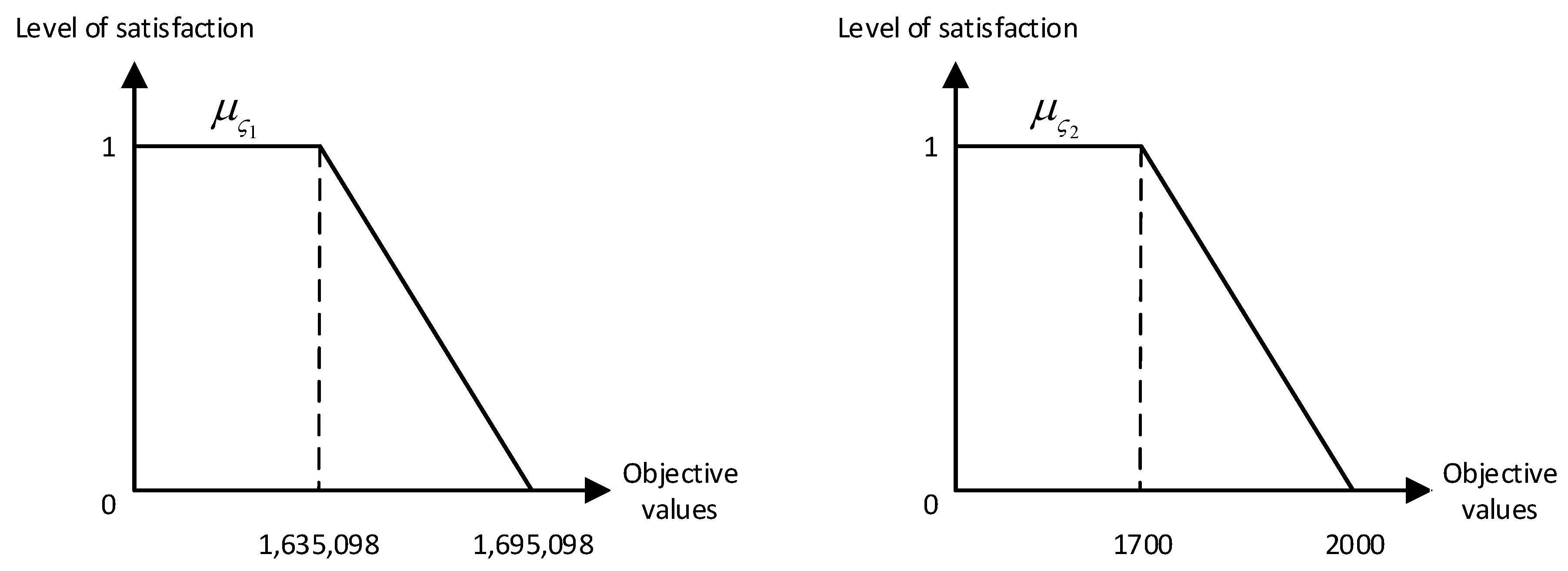
In order to determine model formulation (41), the linear membership functions should be applied for Equations (31) and (32) by testing the range of their objective values.

Table 1. Sensitivity analysis on degree of feasibility ($\alpha$).

$\mathit{\alpha }$	${\mathit{W}}_1^{\mathit{\alpha }-\mathit{PIS}}$ ($)	${\mathit{W}}_1^{\mathit{\alpha }-\mathit{NIS}}$ ($)	${\mathit{W}}_2^{\mathit{\alpha }-\mathit{PIS}}$ (tons)	${\mathit{W}}_2^{\mathit{\alpha }-\mathit{NIS}}$ (tons)
0.1	1,400,372	1,690,324	1700	2400
0.2	1,451,849	1,691,516	1700	2300
0.3	1,483,329	1,692,709	1700	2200
0.4	1,534,811	1,693,903	1700	2100
0.5	1,635,098	1,695,098	1700	2000
0.6	1,656,294	1,696,362	1700	1900
0.7	1,907,492	2,047,492	2200	2600
0.8	1,908,691	2,048,691	2200	2600
0.9	2,069,891	2,259,891	2500	3100

shows the sensitivity analysis on $\alpha$. $W_1^{\alpha -PIS}$ is the optimal objective value (minimum overall system costs) for Equation (31) at each level of feasibility $\alpha$. Similarly, $W_2^{\alpha -PIS}$ is the optimal objective values (minimum negative environmental impact) for Equation (32) at each level of feasibility $\alpha$. Meanwhile, we obtain the optimal decisions $x_1^{\alpha -PIS}$ and $x_2^{\alpha -PIS}$, respectively. $W_1^{\alpha -NIS}$ and $W_2^{\alpha -NIS}$ are derived by plugging the optimal decision $x_2^{\alpha -PIS}$ into Equation (31) and optimal decision $x_1^{\alpha -PIS}$ into Equation (32). For example when $\alpha =0.5$, the minimum overall system cost is $1,635,098 and the maximum overall system cost is $1,695,098. Corresponding annual minimum negative environmental impact is 1700 tons and annual maximum negative environmental impact is 2000 tons. As shown in Figure 2, if the values are smaller than the optimal objective values ($1,635,098 and 1700 tons), then the decision maker is $100\%$ satisfied with the solution. If the values are greater then the worst objective values ($1,695,098 and 2000 tons), then the decision maker is $0\%$ satisfied with the solution. Between the best and the worst objective values, the level of satisfaction decreases as objective value increases since both ${\zeta }_1$ and ${\zeta }_2$ are minimization functions. The goal is to find a balance point between two conflicting objective functions based on the decision maker’s preference. It should be noted that greater $\alpha$ results in more robust solution and hence objective values ($W_1^{\alpha -PIS}$, $W_1^{\alpha -NIS}$, $W_2^{\alpha -PIS}$, $W_2^{\alpha -NIS}$) increase as $\alpha$ increases. When $\alpha$ increases from 0.6 to 0.7, there are significant increases in both overall system costs and negative environmental impact due to network configuration upgrades. This signifies a $\alpha$ smaller than 0.6 would be a good strategy for the company.

5.2. Sensitivity Analysis on ${\theta }_1$ and ${\theta }_2$

The next step is to construct the linear membership functions ${\mu }_{{\zeta }_1}\left(x\right)$ and ${\mu }_{{\zeta }_2}\left(x\right)$ for a given $\alpha$ value. Let’s set $\alpha =0.5$, then the linear membership functions can be expressed as follows:

$${\mu }_{{\zeta }_1}\left(x_1\right)=\frac{1,695,098-x_1}{60,000}\mathrm{and}{\mu }_{{\zeta }_2}\left(x_2\right)=\frac{2000-x_2}{300}$$

where $x_1$ and $x_2$ are the objective values for the crisp model. Notice that

$x_1\in [1,635,098,1,695,098]$ and $x_2\in [1700,2000]$. The denominator of linear membership function is obtained by identifying the range of objective values (e.g., 1,695,098 − 1,635,098 = 60,000 and 2000 − 1700 = 300). Intuitively, the level of satisfaction decreases as $x_1$ and $x_2$ increase because they are minimization functions. The sensitivity analysis on the importance of objective functions is shown in

Table 2. Sensitivity analysis on the coefficient of compensation ($\gamma$).

	${\mathit{W}}_1$ ($)	${\mathit{W}}_2$ (tons)	${\mathit{\mu }}_{{\mathit{W}}_1}$	${\mathit{\mu }}_{{\mathit{W}}_2}$	${\mathit{\lambda }}_0$
$\gamma =0.1$	2,069,891	3100	1	0	0
$\gamma =0.2$	2,069,891	3100	1	0	0
$\gamma =0.3$	2,109,891	2900	0.789	1/3	1/3
$\gamma =0.4$	2,139,891	2800	0.632	0.5	0.5
$\gamma =0.5$	2,139,891	2800	0.632	0.5	0.5
$\gamma =0.6$	2,139,891	2800	0.632	0.5	0.5
$\gamma =0.7$	2,159,891	2700	0.526	2/3	0.526
$\gamma =0.8$	2,159,891	2700	0.526	2/3	0.526
$\gamma =0.9$	2,159,891	2700	0.526	2/3	0.526

Degree of feasibility (α) is fixed at 0.9 and importance of objective functions (θ₁ and θ₂) are fixed at 0.8 and 0.2, respectively.

. ${\theta }_1$ is the importance of the first objective function ${\zeta }_1$ (overall system costs) and ${\theta }_2$ is the importance of the second objective function ${\zeta }_2$ (negative environmental impact). Given the fact that ${\theta }_1$ + ${\theta }_2$ = 1, increasing ${\theta }_1$ while decreasing ${\theta }_2$ indicates the decision maker tends to put more focus on the overall system costs and less focus on the negative environmental impact. In Table 2, $W_1$ is the optimal objective value for ${\zeta }_1$ and $W_2$ is the optimal objective value for ${\zeta }_2$. ${\mu }_{W_1}$ and ${\mu }_{W_2}$ are the level of satisfaction for two objective functions, respectively. ${\lambda }_0$ is the minimum level of satisfaction: ${\lambda }_0=\min ({\mu }_{W_1},{\mu }_{W_2})$. When ${\theta }_1=0.9$ and ${\theta }_2=0.1$, corresponding ${\mu }_{W_1}=1$ and ${\mu }_{W_2}=0$. It indicates that the decision maker is $100\%$ satisfied with the overall system costs and $0\%$ satisfied with the negative environmental impact. This parameter setup makes the solution indifferent to traditional supply chain network system because it does not consider environmental impact and only care about the overall system costs. As ${\theta }_1$ decreases, the decision makers put more and more focus on the environmental impact, therefore, $W_1$ increases and $W_2$ decreases. Notice that ${\mu }_{W_1}$, ${\mu }_{W_2}$ and ${\lambda }_0$ are insensitive to parameter changes in ${\theta }_1$ and ${\theta }_2$. Apparently, minimum satisfaction ${\lambda }_0$ is fairly low across all ${\theta }_1$ and ${\theta }_2$ combinations and this motivates us to investigate how $\gamma$ affect the model solution. From a company’s perspective, they should avoid picking ${\theta }_1=0.9$, ${\theta }_2=0.1$ since the minimum satisfaction level drops to 0. If the company has a budget lower than 1,675,098, then they should pick higher ${\theta }_1$ value and lower ${\theta }_2$ value such as ${\theta }_1=0.8$ and ${\theta }_2=0.2$ so that they can focus more on the financial aspect. On the other hand, if the company wants to generate less negative environmental impact, then they should choose lower ${\theta }_1$ value and higher ${\theta }_2$ value such as ${\theta }_1=0.1$ and ${\theta }_2=0.9$.

5.3. Sensitivity Analysis on $\gamma$

Table 2 includes the sensitivity analysis on the coefficient of compensation ($\gamma$). We fix ${\theta }_1=0.8$, ${\theta }_2=0.2$, $\alpha =0.9$ and only vary $\gamma$ to investigate it’s impact on the solution. The corresponding linear membership functions are shown as follows:

$${\mu }_{{\zeta }_1}\left(x_1\right)=\frac{2,259,891-x_1}{190,000}\mathrm{and}{\mu }_{{\zeta }_2}\left(x_2\right)=\frac{3100-x_2}{600}$$

By comparing Table 2 and

Table 3. Sensitivity analysis on the importance of objective functions (${\theta }_1$ and ${\theta }_2$).

	${\mathit{W}}_1$ ($)	${\mathit{W}}_2$ (tons)	${\mathit{\mu }}_{{\mathit{W}}_1}$	${\mathit{\mu }}_{{\mathit{W}}_2}$	${\mathit{\lambda }}_0$
${\theta }_1=0.1$, ${\theta }_2=0.9$	1,675,098	1800	1/3	2/3	1/3
${\theta }_1=0.2$, ${\theta }_2=0.8$	1,675,098	1800	1/3	2/3	1/3
${\theta }_1=0.3$, ${\theta }_2=0.7$	1,675,098	1800	1/3	2/3	1/3
${\theta }_1=0.4$, ${\theta }_2=0.6$	1,675,098	1800	1/3	2/3	1/3
${\theta }_1=0.5$, ${\theta }_2=0.5$	1,655,098	1900	2/3	1/3	1/3
${\theta }_1=0.6$, ${\theta }_2=0.4$	1,655,098	1900	2/3	1/3	1/3
${\theta }_1=0.7$, ${\theta }_2=0.3$	1,655,098	1900	2/3	1/3	1/3
${\theta }_1=0.8$, ${\theta }_2=0.2$	1,655,098	1900	2/3	1/3	1/3
${\theta }_1=0.9$, ${\theta }_2=0.1$	1,635,098	2000	1	0	0

Degree of feasibility (α) is fixed at 0.5 and coefficient of compensation (γ) is fixed at 0.4.

, it can be found out that the minimum satisfaction level $\left({\lambda }_0\right)$ is more sensitive to the coefficient of compensation ($\gamma$) than the importance of objective functions (${\theta }_1$ and ${\theta }_2$). In Table 2, ${\lambda }_0$ takes value $\frac{1}{3}$ for the most cases which indicates that the model pays more attention to the objective values than the minimum satisfaction levels. In Table 2, ${\lambda }_0$ takes values such as 0, 1/3, 0.5, and 0.526 which are more diverse. Recall two objective functions are conflicting with each other: the first objective function is trying to build facilities with small fixed cost and the second objective function is aiming to build facilities with large fixed cost as they have better sewage and exhaust gas treatment systems. Therefore, solution with minimum satisfaction level greater than 0.5 is good. When $\gamma =0.1$ or $\gamma =0.2$, the solution is indifferent to the traditional supply chain network system because the decision makers only care about the overall system costs and ignore negative environmental impact completely. From a company’s perspective, they should choose $\gamma$ between 0.7 to 0.9 since solutions are balance (${\mu }_{W_1}$ and ${\mu }_{W_2}$ are close to each other) and minimum satisfaction level (${\lambda }_0$) is above 0.5. If the company focuses on cutting the budget, then a small $\gamma$ such as 0.1 is better.

To summarise, Maximum overall system costs and negative environment impact is dependent on the degree of feasibility. The point of balance can be found between the conflicting functions based on decision makes preference and budget for overall system costs. In addition to that the sensitivity analysis shows that there is a trade-off between the two objective functions. The importance of the functions can be changed based on the company’s preferences. Also, the satisfaction level of the company is less sensitive to the objective functions than the coefficient of compensation. This is because building facilities with less environmental impact would require high fixed costs to account for better sewage management systems.

6. Conclusions

Supply chain design is among the most critical decisions in the manufacturing production. Recently, more attention has been paid to the closed-loop supply chain systems as they provide additional profits by collecting end-of-life units and re-manufacturing them for consumption which recovers the value of production. In the traditional supply chain systems, flows start from suppliers, going through manufacturing plants, distribution centers and end at customers. However, closed-loop supply chain systems extend it by collecting defective/used products from customers, classifying them based on the condition, re-manufacturing the recoverable units and sending recovered products back to the customers.

Closed-loop supply chain network design includes many strategic decisions such as network configuration and hence faces significant amount of uncertainties. In this paper, we consider the uncertainties in demand, return, scrap rate, manufacturing costs and environmental impacts. Fuzzy programming works better in terms of modeling and computational efficiency when there are multiple uncertain parameters with rough historical data. One of the contribution for this study is that we proposed a multi-objective fuzzy programming model to copy with uncertainties in the CLSCN. Two conflicting objective functions are minimization of overall system costs and minimization of negative environmental impact. We apply the solution approach proposed by Jimenez et al. to create the crisp model and then integrate different objective functions using the approach proposed by Torabi and Hassini [28,39]. Sensitivity analyses have been conducted on various parameters such as the degree of feasibility $\left(\alpha \right)$, the importance of objective functions $({\theta }_1,{\theta }_2)$ and coefficient of compensation $\left(\gamma \right)$. Managerial insights are provided along with the analyses. It can be observed that: (1) different $\alpha$ values will provide different linear membership functions and a $\alpha$ value smaller than 0.6 should be selected; (2) ${\lambda }_0$ is insensitive to the combinations of ${\theta }_1$ and ${\theta }_2$; (3) By varying $\gamma$, we are able to find a balance solution.

The research is subject to a few limitations which suggest some future research directions: First, time complexity is not addressed in this paper, however, this aspect is really important for large scaled problems and hence developing valid inequalities and heuristic algorithms can be appealing. Second, an efficient approach to capture the statistical properties of uncertain parameters and convert into crisp models is desired. Last but not the least, the choice of raw materials and collection technologies play a big role in environmental impact, therefore considering uncertainties in those two components are also crucial.

References

- Klibi, W.; Martel, A.; Guitouni, A. The design of robust value-creating supply chain networks: A critical review. Eur. J. Oper. Res. 2010, 203, 283–293. [Google Scholar] [CrossRef]
- Pishvaee, M.S.; Rabbani, M.; Torabi, S.A. A robust optimization approach to closed-loop supply chain network design under uncertainty. Appl. Math. Model. 2011, 35, 637–649. [Google Scholar] [CrossRef]
- Hu, Z.; Hu, G. A two-stage stochastic programming model for lot-sizing and scheduling under uncertainty. Int. J. Prod. Econ. 2016, 180, 198–207. [Google Scholar] [CrossRef]
- Hu, Z.; Hu, G. A multi-stage stochastic programming for lot-sizing and scheduling under demand uncertainty. Comput. Ind. Eng. 2018, 119, 157–166. [Google Scholar] [CrossRef]
- Ramaraj, G.; Hu, Z.; Hu, G. A two-stage stochastic programming model for production lot-sizing and scheduling under demand and raw material quality uncertainties. Int. J. Plan. Sched. 2019, 3, 1–27. [Google Scholar] [CrossRef]
- Bertsimas, D.; Thiele, A. Robust and data-driven optimization: Modern decision making under uncertainty. In Models, Methods, and Applications for Innovative Decision Making; INFORMS: Catonsville, MD, USA, 2006; pp. 95–122. [Google Scholar]
- Gülpınar, N.; Pachamanova, D.; Çanakoğlu, E. Robust strategies for facility location under uncertainty. Eur. J. Oper. Res. 2013, 225, 21–35. [Google Scholar] [CrossRef]
- Akçalı, E.; Çetinkaya, S.; Üster, H. Network design for reverse and closed-loop supply chains: An annotated bibliography of models and solution approaches. Networks 2009, 53, 231–248. [Google Scholar] [CrossRef]
- Alem, D.J.; Morabito, R. Production planning in furniture settings via robust optimization. Comput. Oper. Res. 2012, 39, 139–150. [Google Scholar] [CrossRef]
- Hasani, A.; Zegordi, S.H.; Nikbakhsh, E. Robust closed-loop supply chain network design for perishable goods in agile manufacturing under uncertainty. Int. J. Prod. Res. 2012, 50, 4649–4669. [Google Scholar] [CrossRef]
- Hu, Z.; Hu, G. Hybrid stochastic and robust optimization model for lot-sizing and scheduling problems under uncertainties. Eur. J. Oper. Res. 2020, 2, 284. [Google Scholar] [CrossRef]
- Keyvanshokooh, E.; Ryan, S.M.; Kabir, E. Hybrid robust and stochastic optimization for closed-loop supply chain network design using accelerated Benders decomposition. Eur. J. Oper. Res. 2016, 249, 76–92. [Google Scholar] [CrossRef] [Green Version]
- Mirzapour Al-E-Hashem, S.; Malekly, H.; Aryanezhad, M. A multi-objective robust optimization model for multi-product multi-site aggregate production planning in a supply chain under uncertainty. Int. J. Prod. Econ. 2011, 134, 28–42. [Google Scholar] [CrossRef]
- Prajogo, D.; Olhager, J. Supply chain integration and performance: The effects of long-term relationships, information technology and sharing, and logistics integration. Int. J. Prod. Econ. 2012, 135, 514–522. [Google Scholar] [CrossRef]
- Peng, H.; Shen, N.; Liao, H.; Xue, H.; Wang, Q. Uncertainty factors, methods, and solutions of closed-loop supply chain—A review for current situation and future prospects. J. Clean. Prod. 2020, 254, 120032. [Google Scholar] [CrossRef]
- Guan, G.; Jiang, Z.; Gong, Y.; Huang, Z.; Jamalnia, A. A Bibliometric Review of Two Decades’ Research on Closed-Loop Supply Chain: 2001–2020. IEEE Access 2021, 9, 3679–3695. [Google Scholar] [CrossRef]
- Pishvaee, M.S.; Torabi, S.A. A possibilistic programming approach for closed-loop supply chain network design under uncertainty. Fuzzy Sets Syst. 2010, 161, 2668–2683. [Google Scholar] [CrossRef]
- Zarandi, M.H.F.; Sisakht, A.H.; Davari, S. Design of a closed-loop supply chain (CLSC) model using an interactive fuzzy goal programming. Int. J. Adv. Manuf. Technol. 2011, 56, 809–821. [Google Scholar] [CrossRef]
- Jindal, A.; Sangwan, K.S. Closed loop supply chain network design and optimisation using fuzzy mixed integer linear programming model. Int. J. Prod. Res. 2014, 52, 4156–4173. [Google Scholar] [CrossRef]
- Kumar, N.R.; Kumar, R.S. Closed loop supply chain management and reverse logistics-A literature review. Int. J. Eng. Res. Technol. 2013, 6, 455–468. [Google Scholar]
- Amin, S.H.; Zhang, G. A multi-objective facility location model for closed-loop supply chain network under uncertain demand and return. Appl. Math. Model. 2013, 37, 4165–4176. [Google Scholar] [CrossRef]
- Shekarian, E.; Flapper, S.D. Analyzing the Structure of Closed-Loop Supply Chains: A Game Theory Perspective. Sustainability 2021, 13, 1397. [Google Scholar] [CrossRef]
- Shekarian, E. A review of factors affecting closed-loop supply chain models. J. Clean. Prod. 2020, 253, 119823. [Google Scholar] [CrossRef]
- Böhringer, C.; Rutherford, T.F.; Tol, R.S. The EU 20/20/2020 targets: An overview of the EMF22 assessment. Energy Econ. 2009, 31, S268–S273. [Google Scholar] [CrossRef] [Green Version]
- Haddadsisakht, A.; Ryan, S.M. Closed-loop supply chain network design with multiple transportation modes under stochastic demand and uncertain carbon tax. Int. J. Prod. Econ. 2018, 195, 118–131. [Google Scholar] [CrossRef] [Green Version]
- Liang, T.F. Distribution planning decisions using interactive fuzzy multi-objective linear programming. Fuzzy Sets Syst. 2006, 157, 1303–1316. [Google Scholar] [CrossRef]
- Inuiguchi, M.; Ramık, J. Possibilistic linear programming: A brief review of fuzzy mathematical programming and a comparison with stochastic programming in portfolio selection problem. Fuzzy Sets Syst. 2000, 111, 3–28. [Google Scholar] [CrossRef]
- Jiménez, M.; Arenas, M.; Bilbao, A.; Rodríguez, M.V. Linear programming with fuzzy parameters: An interactive method resolution. Eur. J. Oper. Res. 2007, 177, 1599–1609. [Google Scholar] [CrossRef]
- Wang, R.C.; Liang, T.F. Applying possibilistic linear programming to aggregate production planning. Int. J. Prod. Econ. 2005, 98, 328–341. [Google Scholar] [CrossRef]
- Rommelfanger, H.; Słowiński, R. Fuzzy linear programming with single or multiple objective functions. In Fuzzy Sets in Decision Analysis, Operations Research and Statistics; Springer: Berlin/Heidelberg, Germany, 1998; pp. 179–213. [Google Scholar]
- Sakawa, M. Fuzzy Sets and Interactive Multi-objective Optimization; Springer: Berlin/Heidelberg, Germany, 2013. [Google Scholar]
- Fortemps, P.; Roubens, M. Ranking and defuzzification methods based on area compensation. Fuzzy Sets Syst. 1996, 82, 319–330. [Google Scholar] [CrossRef]
- González, A. A study of the ranking function approach through mean values. Fuzzy Sets Syst. 1990, 35, 29–41. [Google Scholar] [CrossRef]
- Parra, M.A.; Terol, A.B.; Gladish, B.P.; Urıa, M.R. Solving a multiobjective possibilistic problem through compromise programming. Eur. J. Oper. Res. 2005, 164, 748–759. [Google Scholar] [CrossRef]
- Zimmermann, H.J. Fuzzy programming and linear programming with several objective functions. Fuzzy Sets Syst. 1978, 1, 45–55. [Google Scholar] [CrossRef]
- Lai, Y.J.; Hwang, C.L. Possibilistic linear programming for managing interest rate risk. Fuzzy Sets Syst. 1993, 54, 135–146. [Google Scholar] [CrossRef]
- Li, X.q.; Zhang, B.; Li, H. Computing efficient solutions to fuzzy multiple objective linear programming problems. Fuzzy Sets Syst. 2006, 157, 1328–1332. [Google Scholar] [CrossRef]
- Tiwari, R.; Dharmar, S.; Rao, J. Fuzzy goal programming: An additive model. Fuzzy Sets Syst. 1987, 24, 27–34. [Google Scholar] [CrossRef]
- Torabi, S.A.; Hassini, E. An interactive possibilistic programming approach for multiple objective supply chain master planning. Fuzzy Sets Syst. 2008, 159, 193–214. [Google Scholar] [CrossRef]
- Fahimnia, B.; Sarkis, J.; Dehghanian, F.; Banihashemi, N.; Rahman, S. The impact of carbon pricing on a closed-loop supply chain: An Australian case study. J. Clean. Prod. 2013, 59, 210–225. [Google Scholar] [CrossRef]
- Krikke, H.; Bloemhof-Ruwaard, J.; Van Wassenhove, L.N. Concurrent product and closed-loop supply chain design with an application to refrigerators. Int. J. Prod. Res. 2003, 41, 3689–3719. [Google Scholar] [CrossRef]
- Selim, H.; Ozkarahan, I. A supply chain distribution network design model: An interactive fuzzy goal programming-based solution approach. Int. J. Adv. Manuf. Technol. 2008, 36, 401–418. [Google Scholar] [CrossRef]
Figure 1.
Closed-loop supply chain configuration
Figure 2.
Linear membership functions for and when .