Article

Data-Driven Sliding Bearing Temperature Model for Condition Monitoring in Internal Combustion Engines

by
Christian Laubichler
1,*,
Constantin Kiesling
1,
Matheus Marques da Silva
2,
Andreas Wimmer
1,2 and
Gunther Hager
3
1
Large Engines Competence Center GmbH, 8010 Graz, Austria
2
Institute of Thermodynamics and Sustainable Propulsion Systems, Graz University of Technology, 8010 Graz, Austria
3
Miba Gleitlager Austria GmbH, 4663 Laakirchen, Austria
*
Author to whom correspondence should be addressed.
Submission received: 31 March 2022 / Revised: 12 May 2022 / Accepted: 18 May 2022 / Published: 22 May 2022
(This article belongs to the Special Issue Tribology in Mobility)

Abstract

:
Condition monitoring of components in internal combustion engines is an essential tool for increasing engine durability and avoiding critical engine operation. If lubrication at the crankshaft main bearings is insufficient, metal-to-metal contacts become likely and thus wear can occur. Bearing temperature measurements with thermocouples serve as a reliable, fast responding, individual bearing-oriented method that is comparatively simple to apply. In combination with a corresponding reference model, such measurements could serve to monitor the bearing condition. Based on experimental data from an MAN D2676 LF51 heavy-duty diesel engine, the derivation of a data-driven model for the crankshaft main bearing temperatures under steady-state engine operation is discussed. A total of 313 temperature measurements per bearing are available for this task. Readily accessible engine operating data that represent the corresponding engine operating points serve as model inputs. Different machine learning methods are thoroughly tested in terms of their prediction error with the help of a repeated nested cross-validation. The methods include different linear regression approaches (i.e., with and without lasso regularization), gradient boosting regression and support vector regression. As the results show, support vector regression is best suited for the problem. In the final evaluation on unseen test data, this method yields a prediction error of less than 0.4 °C (root mean squared error). Considering the temperature range from approximately 76 °C to 112 °C, the results demonstrate that it is possible to reliably predict the bearing temperatures with the chosen approach. Therefore, the combination of a data-driven bearing temperature model and thermocouple-based temperature measurements forms a powerful tool for monitoring the condition of sliding bearings in internal combustion engines.

1. Introduction

Internal combustion engines (ICE) are employed as energy converters in manifold applications such as transportation of goods and people, machinery and power generation [1,2,3,4]. Their widespread utilization is due to advantageous key characteristics such as high power-to-weight ratio, robustness, efficiency, affordability and large-scale fuel supply infrastructure availability [2,3,5]. Global issues such as climate change, environmental pollution and scarcity of resources are currently posing major challenges to engine manufacturers, who must meet the requirements of substantially reduced emissions of CO2 and other greenhouse gases, elimination of pollutant emissions and increased service life of ICEs [3,4,6]. Because the development of entirely new ICE concepts requires extensive research and development work, engine manufactures are focusing on increasing the efficiency of existing ICE technology in the short term [
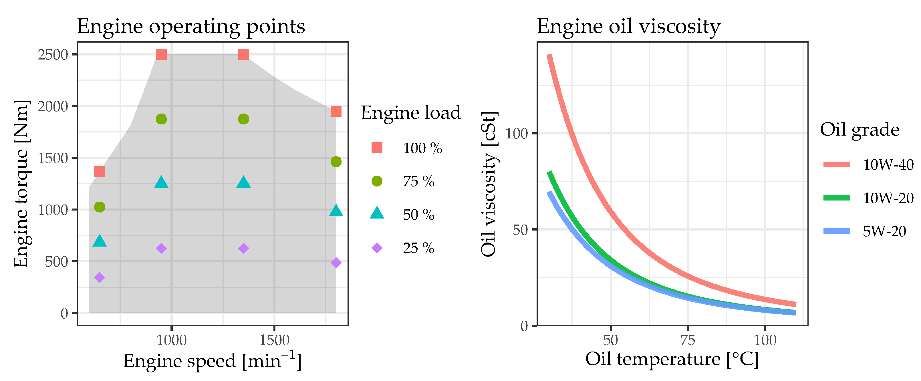
7]. One possible solution employs newly developed low viscosity oils that have the potential to reduce friction and thus increase engine efficiency [7]. However, such oils in turn pose new challenges for sliding bearings in ICEs and their lubrication.
Shafts in multicylinder ICEs, such as crankshafts or camshafts, are generally supported by sliding bearings (also known as journal or plain bearings) [8]. This bearing type is hydrodynamically lubricated, i.e., due to the convergence of the bearing surfaces, their relative motion and the viscosity of the lubricant fluid, a positive pressure is developed that separates the surfaces by a lubricant film [9]. Sliding bearings have a high capability to withstand and dampen shocks, may be divided for easy assembly, come with low space requirements and are insensitive to grime [8,9,10]. Compared to roller bearings, sliding bearings cost less but have higher friction [8]. During normal engine operation, the lubricant film is generally thick enough that the shaft surface does not come into contact with the opposing bearing surface; hence near-zero bearing wear can be expected [9]. During engine start or stop, there is no or too little relative motion, so the lubricant film is either non-existent or too small to completely separate the surfaces. In such cases, metal-to-metal contacts between the shaft and the opposing bearing surface and thus wear can occur [8,10,11,12,13]. Although the use of low viscosity oils has the potential to reduce overall friction, it also decreases the lubricant oil film thickness and therefore increases the risk of metal-to-metal contacts [14,15,16]. This in turn can lead to increased wear, then reduced engine performance and eventually bearing and engine failure [17]. Therefore, appropriate tools for monitoring and assessing the bearing condition will play a key role in increasing engine durability, avoiding critical engine operation and preventing engine failure, thereby avoiding unnecessary engine downtime [17,18,19]. Digital technologies have the potential to accomplish such tasks [20,21].
In the past decades, with the advent and widespread distribution of electronics and integrated circuits, ICE manufacturers have already developed sophisticated digital systems which serve to improve efficiency, power output and emissions behavior of ICEs [21,22,23,24]. Such systems are used to control fuel injection, air/fuel ratio and ignition [25,26,27]; exhaust gas recirculation and variable geometry turbochargers [28,29,30]; and diesel particulate filters and SCR catalytic converters [31]. More recently, advanced digital technologies such as machine learning have enabled an effective and beneficial analysis of the large amounts of data generated by an ever-increasing number of sensors inside ICEs [32,33,34]. The insights gained and the predictive power of such methods can in turn help to meet the high requirements placed on ICEs by using them for applications such as controls [35,36] as well as condition monitoring (CM) and predictive maintenance (PdM) [37,38,39,40,41].
According to Mechefske [42], condition monitoring (and fault diagnostics) of machinery can be defined as “the field of technical activity in which selected physical parameters, associated with machinery operation, are observed for the purpose of determining machinery integrity”. The author further describes that a PdM strategy “requires that some means of assessing the actual condition of the machinery is used in order to optimally schedule maintenance, in order to achieve maximum production, and still avoid unexpected catastrophic failures”. According to Weck [43], CM is divided into the following three subtasks:
1.
Condition detection refers to the acquisition of one or more informative parameters which reflect the current condition of the machinery.
2.
Condition comparison consists of comparing the actual condition with a reference condition of the same parameter.
3.
Diagnosis evaluates the results of the condition comparison and determines the type and location of failure. Based on the diagnosis, compensation measures or maintenance activities can be initiated at an early stage.
Besides the diagnosis to determine the type and location of failure, there are other evaluation goals for a CM system as well. Beyond the diagnosis task, Vanem [44] and Mechefske [42] introduce prognostics as a task that provides information about the possible future of the condition of the machinery. Furthermore, condition monitoring can generally be classified as either permanent or intermittent monitoring [43,45].
Existing literature proposes several measurement parameters that can help in detecting the sliding bearing condition. Two main categories are observed. First, there are significant parameters such as vibration, acoustic emission and oil contaminants [46,47,48,
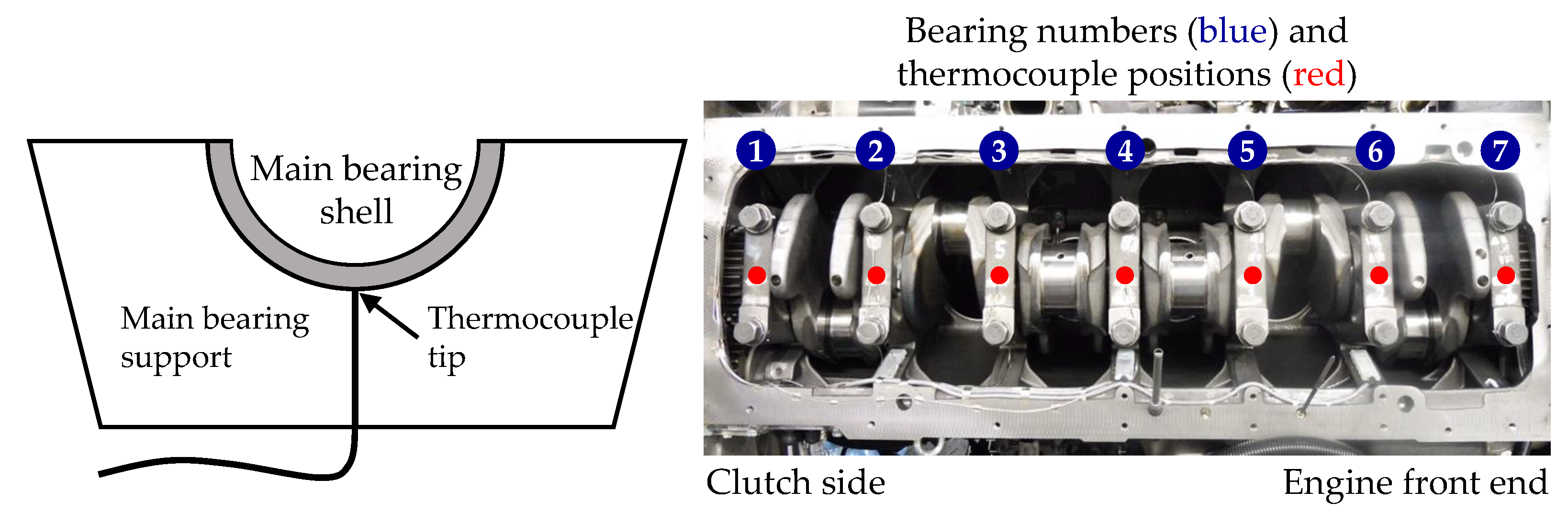
49], which can be measured at a certain distance from the bearing. Second, there are informative parameters that have to be measured directly at or inside the bearing. These include bearing temperature [19,50,51], bearing deformation and vibration [19], oil film temperature [19,51], oil film pressure and thickness [50,52,53] and metal-to-metal contact [47]. With the second category, information can be obtained about the condition of each individual bearing, and the signal quality is higher and transient response faster in case of a rapid change in bearing condition compared to measurement parameters acquired at a distance from the bearing [51,54]. At the same time, it likely requires a larger effort for instrumentation due to the restricted access to the bearings and the need to not influence bearing functionality [7]. In the existing literature, bearing temperature measurement with instruments such as thermocouples has proven to be a reliable, continuous, fast responding measurement method that is comparatively simple to apply [15,50,55]. With these characteristics, the method is particularly useful to diagnose bearing failure modes which lead to a rapid change in bearing temperature [47,56,57].
A straightforward approach to condition comparison of bearing temperature values would simply employ a global temperature limit which may not be exceeded during engine operation. With this approach in particular, anomalies in bearing temperature behavior may not be detected if the defined temperature limit is not reached during the anomaly. On the contrary, a bearing temperature model that incorporates the current engine operation would enable the identification of anomalies in bearing temperature as soon as the measured temperature is outside the limits of a comparatively small tolerance range around the predicted model value. For such a model, transient engine operation poses a specific challenge: Due to the thermal inertia of the engine components and the engine operating media, the bearing temperature reacts slowly to swift changes in engine operating conditions such as engine speed and engine torque. However, this is beyond the scope of this paper with its focus on steady-state engine operation. There are two main types of approaches for deriving a bearing temperature model: data-driven approaches and physics-based approaches (also referred to as model-based or model-driven) [44]. While the latter apply physical domain knowledge to formulate a mathematical model of the monitored machinery condition [58], data-driven approaches simply utilize the inherent information in the available data [44]. Finally, the combination of a physics-based and a data-driven approach is often referred to as a hybrid approach [44].
Today artificial intelligence (AI) and in particular machine learning (ML) form the backbone of data-driven approaches. Although AI and ML emerged in recent times, their origins date back to the 1950s and even earlier [59,60]. Machine learning refers to the ability of an AI system to extract its own knowledge from raw data [60]. Therefore, statistical learning methods such as (linear) regression models are usually included in ML [60,61,62]. For machine fault diagnosis, CM or PdM data-driven methods have been proven to work in various engineering application scenarios [63,64,65], yet the simple application and training of data-driven methods is usually not straightforward because proper data and knowledge are required to train a suitable model. Consequently, it is common to use more controllable experimental data rather than data from a real-world application for model training [58]. However, by taking into account the application-specific background and the underlying structure of the experimental data, it is possible to derive a model that can be generalized for real-world applications or at least taken as the basis for further developments.
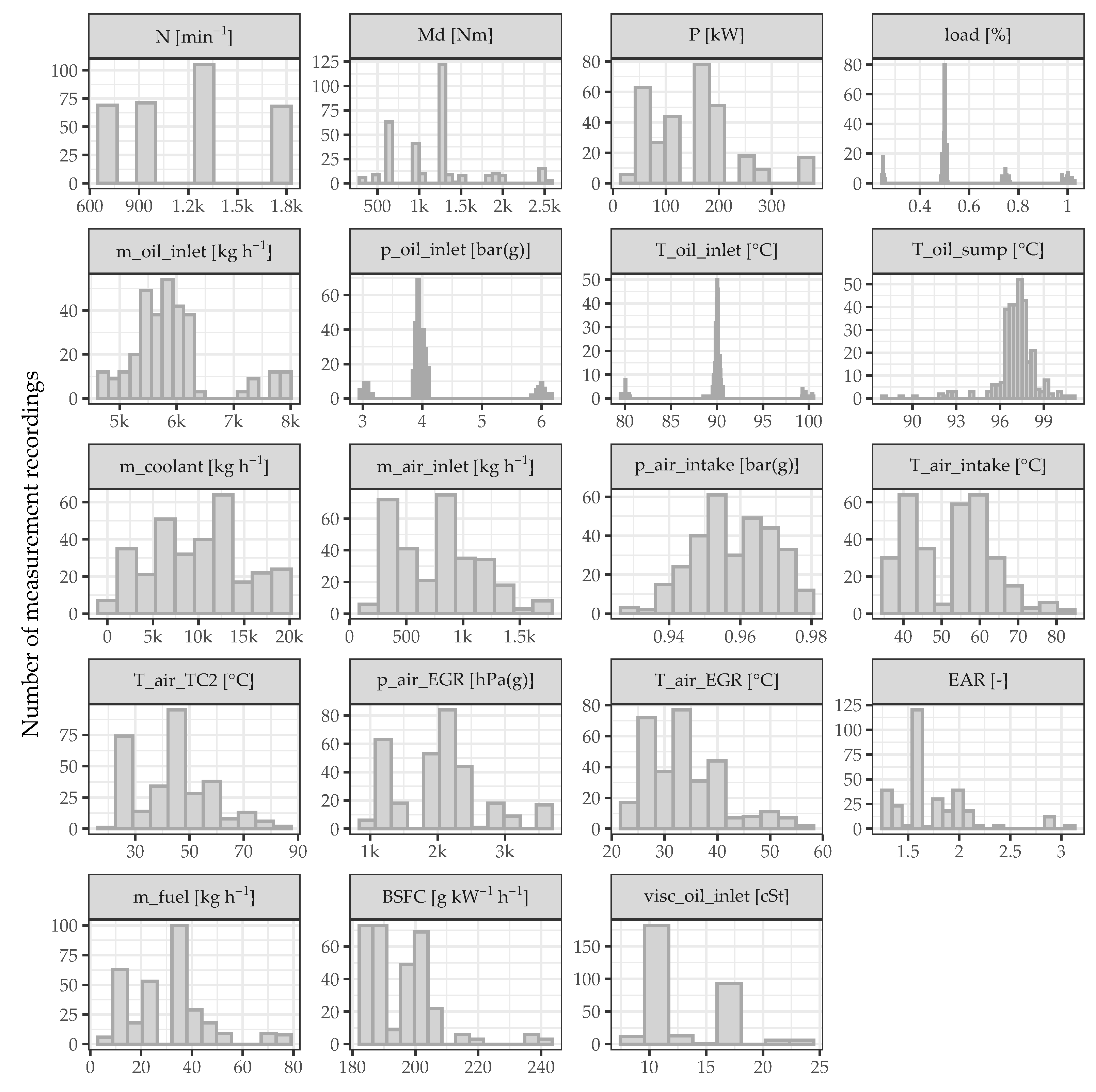
The goal of this paper is to demonstrate that the combination of a data-driven bearing temperature model and thermocouple-based temperature measurements forms a powerful tool for monitoring the condition of sliding bearings in ICEs. The data-driven model of the crankshaft main bearing temperatures under steady-state engine operation is derived based on experimental data. In order to obtain a model that is realistic for real-world applications, only measured or calculated parameters that would also be available on a production engine are considered as model inputs. In Section 2, information on the experimental investigations is provided and the acquired data are analyzed. In addition, the requirements for a suitable data-driven model, the considered ML methods as well as the model training and selection approach are discussed. The results of the modeling process are then presented and analyzed in Section 3. Finally, the main conclusions and possible next steps are discussed and summarized in Section 4 and Section 5.

2. Materials and Methods

2.1. Experimental Investigations

To generate a measurement database, experimental investigations with a test engine were carried out on one of the Large Engines Competence Center’s (LEC) engine test beds at the Graz University of Technology campus. The engine under study is an MAN D2676 LF51 in-line six-cylinder diesel engine, which has a displacement of approximately 12.4 dm3 and is used for heavy-duty applications. During fired engine operation, a VA Tech Elin EBG GmbH Indy 80/4P/5500 dynamometer with a pendulum stator acted as a brake and thus controlled the engine speed level. The engine was operated and monitored with the test bed automation system PUMA Open version 1.5.3 from AVL List GmbH (Graz, Austria). Some engine parameters were directly measured and retrieved via the engine’s electronic control unit (ECU). The additionally applied measurement technology, the experimental setup and the engine operating strategy are summarized below. A more detailed description of the experimental methodology can be found in [7].
Comprehensive external conditioning systems for coolant and lubricating oil and for fuel, charge air and ambient air were employed to ensure defined and accurately reproducible engine operating conditions and to allow the independent adjustment of specific parameters. All relevant parameters such as engine torque and speed as well as media temperatures, pressures and flow rates were measured and recorded with measuring instruments and a data acquisition system. The measuring instruments applied are specified in Section 2.2 (data selection process, cf. Table 1). The temperatures of the seven crankshaft main bearings were measured with type K thermocouples (Class 1 accuracy) fitted through a bore in the bearing support whose measuring tip is in contact with the external surface of the bearing shell. Figure 1 schematically illustrates this measurement setup for a single crankshaft main bearing. The instrumented bearings are numbered one to seven, starting from the clutch side. No measurements of bearing #2 are available due to sensor failure.
The operating points used for the engine tests were based on the sixteen specific operating points illustrated in Figure 2, which include various combinations of engine speed and engine torque. Nearly the entire engine operating map is covered, where engine load is defined as the percentage of the maximum available brake torque at a defined engine speed. After adjustment of each operating point, a settling time of approximately 15 min was observed to ensure that all relevant measurement parameters were in a steady state. These parameters are recorded and averaged over a period of 30 s. In order to examine and ensure the repeatability of the measurements, three consecutive recordings were performed at each investigated operating point.
At the 50 % engine load operating points, oil inlet temperature and inlet pressure were varied individually and independently with the oil conditioning system. Oil temperature was varied from 90 °C (standard temperature) to 80 °C and 100 °C and oil pressure was varied from 4 bar(g) (standard pressure) to 3 bar(g) and 6 bar(g). All parameter variations described above were carried out with three different lubricant oil viscosity grades, whose setting was achieved through oil changes at engine standstill. The employed grades were SAE 10W-40, 10W-20, and 5W-20. Due to testing time limitations, the oil temperature variation was not carried out with the viscosity grade 5W-20. The viscosity of each oil in relation to the oil temperature is shown in Figure 2 (values provided by oil supplier).

2.2. Data Selection and Model Requirements

The data include a total of 313 temperature measurements per bearing that originate from 105 different operating points (for two operating points, only two repetitions were valid). Although a large number of parameters were measured during the engine tests, only specific parameters are used to model the bearing temperatures under steady-state operation. The modeled bearing temperature should solely depend on engine parameters that would be available on a production engine as well. Furthermore, by selecting parameters whose influence on bearing temperature can be ruled out on the basis of physical considerations, there is the risk of the model relying on parameters that correlate with the bearing temperature but do not cause it. The following considerations have also affected data selection:
  • Due to the applied conditioning systems, coolant-related parameters such as pressure and temperature at inlet or outlet are constant and therefore irrelevant to modeling. This also applies to ambient air temperature. The coolant mass flow, however, is a measurement result that varies according to the applied engine operating point. Therefore, it is considered as a model input candidate.
  • Indication system-based measurements such as in-cylinder pressures and key figures derived from them are not considered because they are usually not available on a production engine.
  • Linear transformations of a single measured or calculable parameter are not used for modeling. For example, the break mean effective pressure (BMEP) is a linear transformation of the brake torque, which is considered to be available from the ECU of a production engine. Parameters that are calculated from multiple other parameters (e.g., brake-specific fuel consumption is calculated from fuel mass flow and engine power) are considered as model input candidates.
Taken together, the measured or calculated parameters listed in Table 1 are considered for modeling the seven crankshaft main bearing temperatures. With the bearing-related information, i.e., the targeted temperature as well as the bearing identification parameter, it is possible to distinguish between the bearing positions during modeling. As an additional model input candidate, the oil type information is indirectly included via the temperature-dependent oil viscosity curves shown in Figure 2, where for each measurement, the oil temperature at the engine inlet is used as reference. To avoid any circular reasoning, it was decided not to use the crankshaft main bearing temperatures as references for a bearing-specific viscosity approximation, but rather the technically most proximate one. Moreover, this viscosity information could be adapted for use in a production engine as well.
Figure 3 shows all available temperature measurements, where each temperature profile corresponds to an associated measurement recording. As already mentioned, the temperature values for bearing #2 (MB2) are missing (for graphical representation, these values were linearly interpolated, but the interpolation must be considered inaccurate). As a result, the bearing position-related information is considered as a nominal variable, i.e., there is no ranking of the positions. To avoid an arbitrary joint numerical encoding (e.g., a single bearing variable taking values from 1 to 7), so-called one-hot encoding (also referred to as full dummy encoding) is used. As described in Table 1, by using one-hot encoding, each bearing position is a single Boolean variable (i.e., true or false), which is then binary encoded for modeling (i.e., 1 or 0). Through this encoding, it is possible to derive a single model that includes all bearing positions and can serve as reference during condition comparison of newly measured bearing temperatures.
Based on Figure 3, it also appears that the peripheral bearings #1 and #7 generally exhibit a significantly lower temperature level than bearings #3 to #6. This is likely because the thermal load is lower at the ends of the crankshaft, where there is only one neighboring crankpin and where heat dissipates more quickly due to a considerable temperature gradient towards the crankcase. All six observed bearing-related temperature distributions are similar but have shifted centers. The single temperature profiles are smooth and appear shifted by an individual base level. This is another motivation for using the one-hot encoded bearing position. However, all curves do not behave uniformly, especially at bearing #5.
The distributions of the measured and calculated parameters shown in Figure 4 do not provide a uniform picture either. Since the parameters do not change between the bearings, they are included once (i.e., 313 observations per plot). Due to the experimental design, several parameters have a rather discrete or multimodal distribution. Furthermore, some parameters distributions are skewed or heavy-tailed.
As shown in Figure 5, some parameters are also correlated with each other. The Pearson correlations in the left correlation matrix plot are calculated using the raw values and indicate the linear relationship between two parameters. The Spearman’s rank correlations are based on the parameter rankings and indicate how monotonic the relationship between two parameters is. Both correlation matrices show a similar picture and indicate so-called multicollinearity and redundancy of several parameters. For example, while all air temperature-related parameters are positively correlated, the intake air pressure at intake manifold has a (weak) negative correlation with all of them. As might also be expected, load and engine power are positively correlated with engine torque.
However, if there are non-monotonic relationships, both Pearson and Spearman-type correlations can miss out on important associations [67]. In contrast, Hoeffding’s D [68] is a general and robust similarity measure for detecting dependencies [67]. Dendrograms from hierarchical cluster analyses of the Pearson correlation and the Hoeffding’s D similarity measures are shown in Figure 6. The further right a split is in a dendrogram, the stronger the correlation/dependency between two subsequent clusters. Both reveal a similar basic relationship structure between the engine operation parameters. But they also indicate different relationships for some parameters. While m_oil_inlet and p_oil_inlet are only strongly (linearly) correlated with each other (cf. Figure 5), m_oil_inlet is closer to p_air_intake and visc_oil_inlet in terms of Hoeffding’s D.
While collinearity makes it difficult to interpret the effect of individual model parameters, it does not affect predictions that are made on datasets similar to those on which a model was fit [67]. Therefore, whether collinearity is problematic is closely related to the actual aim for which a data-driven model should be used.
Deciding between interpretable model types and black boxes or between parsimony and complexity are two of the many choices that need to made when deriving a model [67]. While a simple and rather inflexible method is advantageous if inference is the goal of a data-driven approach, the interpretability of a model does not matter if the focus is on prediction [61]. But complex and highly flexible ML methods do not necessarily result in more accurate predictions because they also have a higher risk of overfitting [61]. For this reason, a proper model training strategy is required, especially for highly flexible ML methods. In the event that a black-box model eventually yields the best results, however, it is still possible to gain insights by developing an interpretable approximation to the black-box model [67].
First and foremost, the data-driven model for monitoring the bearing temperatures should be capable of accurately predicting the temperature values based on the engine parameter inputs. In terms of machine learning, a predictive model attempts to predict a given target using other variables (or features) in the dataset as inputs [70]. Since the target is given, such a task is usually referred to as supervised learning. On the contrary, unsupervised learning lacks a target and aims to better understand and describe a given dataset [70]. Depending on whether the target is a numeric (continuous) or a categorical (discrete) outcome, supervised learning is further divided into regression tasks and classification tasks, respectively [70]. Since the bearing temperature is a numeric variable, ML methods for regression tasks may basically be applied.

2.3. Machine Learning Methods

From ordinary linear regression to highly complex deep neural networks, there are various ML methods available to address a regression problem. Yet since there is no single best method for all possible datasets, it is challenging to select the best approach [61]. In addition to the considerations regarding the model aim discussed above, the available data also inherently influence the choice of potential methods. This paper examines three different ML methods: linear regression (with and without lasso regularization), gradient boosting regression and support vector regression. They differ in their interpretability as well as flexibility, whereas flexibility is significantly affected by so-called hyperparameters—the “adjusting screws” of an ML method that require sophisticated tuning during model training with the so-called training data.
Many different software solutions are available for the computational implementation of a machine learning project. For this paper, model training is basically carried out and controlled using the statistical programming language R [71]. Furthermore, seamless integration of Python [72] libraries such as scikit-learn [73] has been achieved through a self-implemented solution based on the R packages reticulate [74] and R6 [75].

2.3.1. Linear Regression and Regularization

Linear regression is a fairly simple method that often provides an adequate and interpretable description of how features affect a target [62]. The (multiple) linear model (LM) has the form
f x = β 0 + j = 1 p β j · x j ,
where x = ( x 1 , , x p ) T is the p-dimensional vector of input variables and β = ( β 0 , , β p ) T are the corresponding model coefficients [62]. The most popular method for obtaining estimates of the model coefficients is the least squares method, which aims to minimize the residual sum of squares
RSS β : = i = 1 n y i f x i 2 ,
where the (training) data consist of n instances (or observations) of targets y i and feature vectors x i = ( x i 1 , , x i p ) T , i = 1 , , n .
An LM has no hyperparameters to tune and is easy to fit (i.e., there is a unique solution of the least squares minimization problem). However, the set of features and the inherent model formula have to be set beforehand. Often stepwise feature selection techniques (e.g., those based on statistical hypothesis tests) are applied to find the most important features, but these techniques are associated with major problems and should be avoided [67]. In contrast, the so-called lasso [76] is a regularization method that shrinks coefficients towards zero by adding the penalty term λ · j = 1 p β j to the RSS minimization problem (2), where the tunable hyperparameter λ 0 determines the strength of the shrinkage penalty. With the lasso, all features are considered, but if λ is large enough, some coefficients are forced to be exactly zero and a feature selection is performed [61]. For a fair comparison of the features, they have to be on similar scales and thus an initial standardization is required (i.e., center a variable by its mean and divide it by its standard deviation) [77].
In this paper, two fixed LM structures (both realized directly in R) are considered for predicting the bearing temperatures:
  • An LM including all available engine parameters (cf. Table 1) as well as the categorical bearing position
  • A naive reference LM that includes only the categorical bearing position (equivalent to taking the average temperature of each bearing from the training data)
For a sparser representation of the bearing temperatures, an LM with lasso regularization is also evaluated. In this paper, the R package glmnet [78] was chosen for the lasso computations because it allows for individual penalty factors per coefficient. In this way, the shrinkage of a coefficient can be omitted (i.e., the corresponding variable is always included in the model) or even more strongly forced [77,78]. Based on the underlying data structure and the discussed model aim, the bearing position identifiers (MB1, …, MB7) are not penalized. All engine parameters (cf. Table 1) are penalized equally except for parameters that are directly calculated from other parameters, which are additionally penalized by the number of other parameters involved. Therefore, engine power P (product of N and Md) and BSFC (calculated with m_fuel and P) are penalized two and three times, respectively.

2.3.2. Gradient Boosting Regression

Gradient boosting (GB) regression is based on decision trees. A decision tree is a summary of rules used to split the feature space into different regions/partitions [61]. Although a single decision tree is hardly capable of adequately modeling a regression problem, many of these weak trees can be aggregated into a potentially very powerful predictive model (a “committee”) using a so-called ensemble method [61,62]. With GB, the regression tree ensemble learns sequentially, i.e., each tree learns from the previous one by being fit on the residuals of the previous tree (i.e., the differences between actual and predicted target values), thereby improving the ensemble [70]. The aggregated predictive model of B trees has the form
f x = b = 1 B f b x ,
where x = ( x 1 , , x p ) T is the p-dimensional input vector and each f b is a single decision tree that was fit on the residuals from f b 1 [70]. This GB approach minimizes the mean squared error loss function and is considered as a gradient descent algorithm that can be generalized to other loss functions as well [70].
There are many software solutions available with different variants of GB algorithms. For this paper, the widely used XGBoost library (short for eXtreme Gradient Boosting) [79] is applied via its scikit-learn API. XGBoost offers a variety of tunable hyperparameters including additional regularization terms. Table 2 summarizes the hyperparameters used for tuning.

2.3.3. Support Vector Regression

Support vector regression (SVR) is essentially an adaptation of the support vector machine (SVM) that is intended for binary classification problems. SVR aims to find a function in the feature space that should not deviate from each target by more than a tolerance margin ε and at the same time is as flat as possible [80]. While errors less than ε are not penalized, errors greater than ε are penalized with an additional hyperparameter C > 0 . As a result, there is a trade-off between the flatness of the function and the tolerance for larger errors [80]. The corresponding loss function for an error ξ is therefore called ε -insensitive loss function ξ ε : = max ( 0 , ξ ε ) [80]. This type of SVR is usually referred to as ε -SVR [80].
Analogous to the SVM, the real strength of the SVR comes from using the so-called kernel trick, in which the feature space is implicitly projected into a higher-dimensional space, where the problem may be easier (linear) to solve. In this way, it is also possible to model nonlinear target behavior in the original feature space. For a p-dimensional input vector x = ( x 1 , , x p ) T and based on the data consisting of n feature vectors x i = ( x i 1 , , x i p ) T , i = 1 , , n , the SVR model has the form
f x = β 0 + i = 1 n α i · k ( x i , x ) ,
where β 0 is an intercept term, α i , i = 1 , , n , are instance-related coefficients that need to be optimized with regard to the targets and k is the kernel function [81]. There are various kernel types with different properties and even additional hyperparameters [80,81]. This paper considers the linear kernel k x i , x = x i · x and the radial basis function (RBF) kernel k x i , x = exp γ · x i x 2 , γ > 0 . While the linear kernel is very simple, the RBF kernel actually projects into an infinite-dimensional space. Thus in contrast to the linear kernel, the interpretability of the model in respect of the feature space is lost with the RBF kernel.
The kernel selection is considered as an additional hyperparameter that is tunable. The SVR is evaluated using the scikit-learn implementation [73], and Table 3 summarizes the hyperparameters used for tuning. Since SVR is a distance-based method like the lasso LM, similar feature scales (e.g., via standardization) are required.

2.4. Model Training and Selection

A good predictive model does not need to perform well on the already known training data, but it should accurately predict previously unseen test data [61]. Therefore, it is of interest to find the method that yields the lowest test error (or loss) rather than the lowest training error [61]. There are various measures for assessing the prediction error/loss of an ML method. This paper uses the mean squared error (MSE) for training and evaluation of the ML approaches presented above. Later, the mean absolute error (MAE) will also be used for comparison purposes. For n pairs of actual target values y = ( y 1 , y n ) T and model predictions y ^ = ( y ^ 1 , , y ^ n ) T = ( f ^ x 1 , , f ^ x 1 ) T , they are defined as follows:
MSE y , y ^ : = 1 n i = 1 n y i y ^ i 2 MAE y , y ^ : = 1 n i = 1 n y i y ^ i
For better interpretation in terms of the original units, the root mean squared error (RMSE), RMSE y , y ^ : = MSE y , y ^ , will also be reported in some instances.
In ML, the entire dataset is usually split into data for training and data for testing that is not used during model training to accommodate the idea of unseen test data. However, there are some pitfalls to this approach. On the one hand, if the model was trained on data completely different from what it is tested on, the risk is high that the results are not accurate. On the other hand, if there is any information leakage from the test data to the training data, the performance evaluation on the test data might be positively biased. An example of such information leakage is the use of all data for standardizing. Therefore, proper model training requires the performance of such steps solely using the training data. This also applies to the data analyses presented in Section 2.
To evaluate the performance of the final bearing temperature model, the data are randomly split into approximately 75 % training data (235 measurement recordings) and 25 % test data (78 measurement recordings). Since the random sampling is performed on the 313 measurement recordings, all six bearing measurements from one measurement recording are in the same split. In addition, the random sampling is restricted so that all two or three measurement recordings of each of the 105 engine operating points are in the same split (i.e., grouped sampling to ensure that probably very similar measurements are kept together) and the training and test data both have similar temperature distributions (i.e., stratified sampling on the mean bearing temperature per measurement recording).
Only the training data are used to tune all the ML approaches and find the best predictive model. To tune the hyperparameters of an ML method, it is again necessary to compare and evaluate the performance of different hyperparameter settings on previously unseen data. A so-called k-fold cross-validation (CV) is often used for hyperparameter tuning. For the CV, the training data are split into k equally sized parts, and each part is used once for validation (testing) iteratively while training is performed using the k 1 others. The average of the k errors, the CV error, indicates the hyperparameter setting with the best overall performance. A strategy is also required to define a set of hyperparameter candidates in the first place. Two common approaches are the grid search and the random search. While the grid search involves evaluating all combinations of a predefined hyperparameter grid with a CV, the random search consists of random sampling of a fixed number of combinations from specified hyperparameter distributions.
However, CV also has its potential pitfalls [82]. For example, the approach discussed above (for hyperparameter tuning) may yield optimistically biased estimates of the generalization error of a model [83]. The entire process of tuning a model should be seen as an integral part of model fitting and be validated as well [83] including all preprocessing steps. To this end, complete modeling procedures (or pipelines) must be evaluated and compared.
In this paper, the bearing temperature model is derived using a so-called repeated nested cross-validation. Figure 7 illustrates a nested CV process. During each outer CV iteration, the currently available training data are again split for the inner CV. While the inner CVs are used to train and tune the modeling procedures, the outer loop is used to compare their performance. Analogous to the basic train–test split described above, all outer and inner CVs samplings are again grouped by engine operation points and stratified by the bearing temperature values. To derive reliable generalization error estimates, the entire nested CV procedure is repeated multiple times. The lowest mean CV error determines the most suitable modeling procedure for the bearing temperature CM model. This modeling procedure is then fit again on the entire training data before it is assessed on the unseen test data.
The entire nested CV procedure has been self-implemented in R, including support for parallel computing. In combination with the R-based solution, which allows seamless integration of Python, it is possible to evaluate the R and the Python procedures with random but identical CV splits. With this CV implementation, a nested CV is repeated 25 times to derive the results presented below. In the course of this, five folds are used for all outer as well as inner CVs. Since the hyperparameter search is an integral part of each modeling procedure, algorithms suited for each ML method are applied. While glmnet’s default log scale-based 1D grid search [78] is used for the LM with lasso regularization, scikit-learn’s [73] RandomizedSearchCV (with 1000 samples) and GridSearchCV (with 1456 combinations) are used for the GB regression and the SVR, respectively.

3. Results

3.1. Cross-Validation Results and Model Selection

Figure 8 presents the distributions of the CV errors over the 25 nested CV repetitions. Both the MSE-based CV errors (i.e., the minimization target during training) and the CV-related MAEs are provided. The two plots show that for all CV repetitions, the SVR modeling procedure best predicts the bearing temperatures. Considering the temperature range from approximately 76 °C to 112 °C, considerably small CV errors of less than 1 °C (both RMSE and MAE) are achieved with the SVR. The XGBoost regressions perform worse than the LMs using all engine parameters (LM_all) and the lasso-regularized LMs (LM_lasso). Compared to the other methods, the results of the GB approach are also not that stable. Nevertheless, all these plotted methods are able to predict the bearing temperatures well. For graphical reasons, the results of the LM that relies on the categorical bearing position only (LM_bearing) are not displayed. As listed in Table 4, this crude approach yields stable yet much higher errors than all other ML methods.

3.2. Model Assessment on Test Data

To assess the performance of the SVR on the test, the entire modeling procedure is carried out again using all training data. Evaluated by means of a 5-fold CV, the grid search yields the optimal hyperparameters reported in Table 5.
As shown in Figure 9, the SVR also performs very well on the previously unseen test data. There are only minor errors and the residuals do not show any patterns, so the model has a similar predictive accuracy throughout the entire temperature range. The largest residuals of the test data predictions are observed with regard to bearing #5. Moreover, the error comparison in Table 6 shows that the test errors are in accordance with the CV errors. The higher errors for bearing #5 are also in agreement with the graphical observations of the bearing temperature profiles (cf. Figure 3).
Since the RBF kernel is chosen, the SVR does not allow for a direct interpretation of the feature’s importance. The LM with lasso regularization (also trained on the entire training data) is strongly correlated with SVR results (Pearson correlation of 0.9881). This also applies to the previously derived CV results, where the correlation between the predictions of these two ML methods ranges between 0.9871 and 0.9905. The LM with lasso regularization (with an optimal hyperparameter λ = 0.0237 ) allows a direct interpretation of the features. The selected variables (nonzero coefficients) form the simple bearing temperature model
T _ MB = 13.2245 5.7486 · MB 1 0.2673 · MB 3 + 1.8001 · MB 4 + 0.7950 · MB 5 + 1.7327 · MB 6 2.5297 · MB 7 + 0.0083 · N + 2.0051 · load 0.0006 · m _ oil _ inlet + 0.8787 · T _ oil _ inlet 0.0644 · T _ oil _ sump + 0.0034 · m _ air _ inlet 4.7267 · p _ air _ intake + 0.3624 · visc _ oil _ inlet ,
where the coefficients correspond to the non-standardized inputs of the engine parameters. For proper interpretation of the interrelationships, it is necessary to rely on currently available information only. Although not very different from the entire dataset, the Pearson correlations and the Hoeffding’s D statistics of the engine parameters for the training data only are provided in Figure 10. Except for the strong positive correlation between N and m_air_inlet, there are no other strong correlations among the model variables due to the lasso regularization. Replacing a model variable in the LM equation (6) above with another non-included engine parameter that is only correlated to that included model variable would not change the predictive performance of the model greatly. Therefore, replacing m_oil_inlet with p_oil_inlet would not significantly change the model results (if the unit-related coefficient is compensated). As to be expected, T_oil_inlet has an effect on the bearing temperature and is (weakly) related to visc_oil_inlet. However, no further dependencies on T_oil_inlet are observed. All other selected features of the LM_lasso model (6) are related with multiple non-included engine parameters. For this reason, a final judgment on their individual importance would require additional (statistical) investigations.

4. Discussion

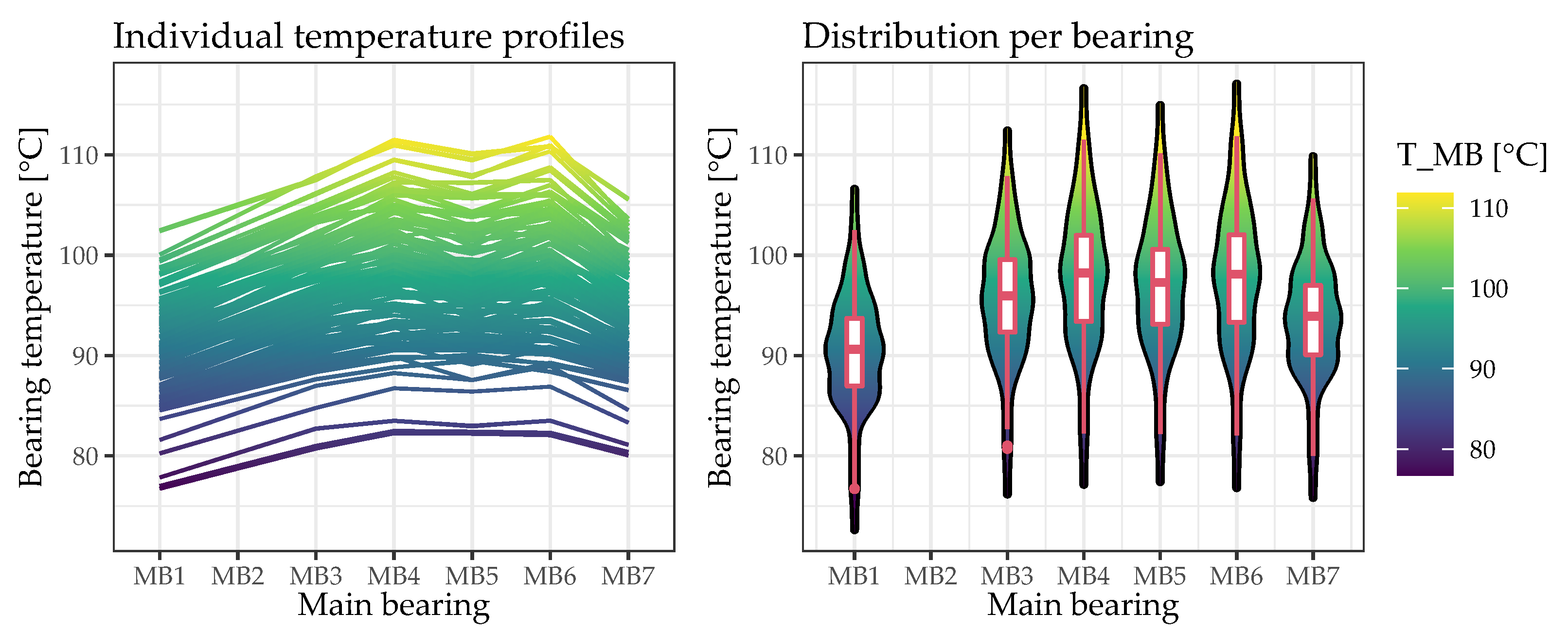
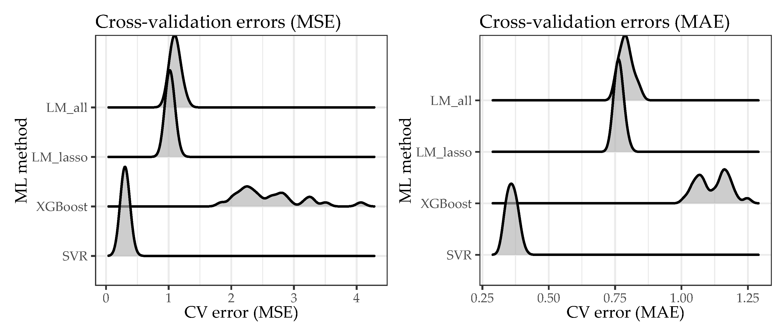
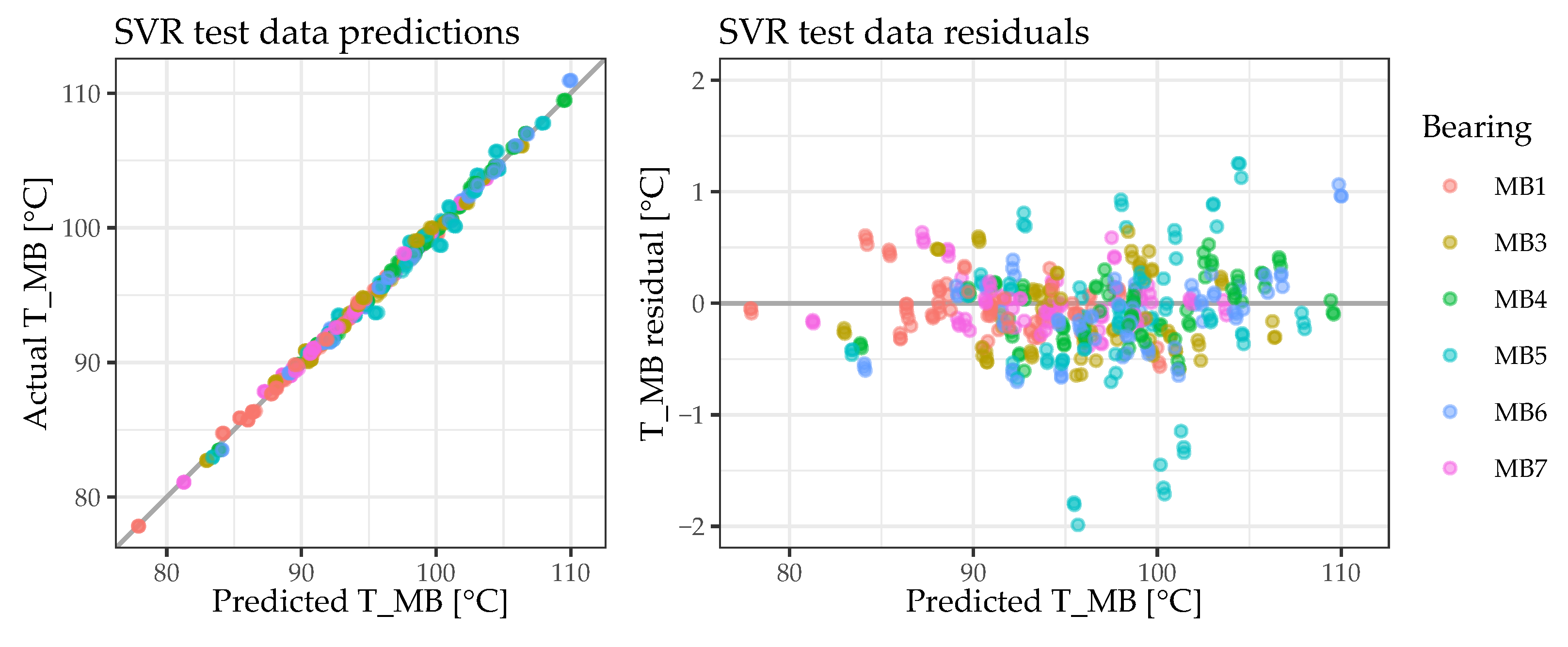
Considering the temperature range from approximately 76 °C to 112 °C, with a prediction error of 0.3995 °C (RMSE on previously unseen test data), the results presented above show that it is possible to reliably predict bearing temperatures on the basis of engine operation parameters. However, the results also demonstrate that there is often a trade-off between the interpretability and the predictive quality of a data-driven approach. While the best model obtained (an SVR with a radial basis kernel) does indeed perform excellently as it predicts the bearing temperatures on the basis of engine operation parameters, it does not allow for a direct interpretation of their importance. Nevertheless, given the wide range of ML methods applied, it has also been demonstrated that a simpler and more easily interpretable approach (the LM with lasso regularization) serves as an understandable approximation of the best model obtained. Since only a subset of the engine parameters is used for predicting the bearing temperatures, the simpler approach would also be more robust to potential sensor failures.
Considering the comparatively small amount of data available for an ML application, more data will be acquired in a follow-up measurement campaign to improve and validate the derived data-driven CM model as well as to acquire data from the currently missing bearing position #2. Hence, the bearing position correlation and encoding will be reevaluated. With the insights already gained (especially from the interpretable ML approach), meaningful data can be efficiently acquired and very low or high bearing temperatures can be specifically studied.
To further improve the performance of the predictive model, additional ML methods such as kernel ridge regression or random forests could be evaluated as well. It might also be beneficial to enhance the LM approaches by using parameter transformations or interaction terms. Linear additive models, for example, also permit modeling of the nonlinearity of certain features. Additional preprocessing steps such as principal component analysis may help to further improve the performance of a modeling procedure. All these model types and methods could easily be implemented in the previously created modeling pipeline. Of course other ML methods such as artificial neural networks could improve the predictions as well, yet such methods usually require even greater training effort, which would necessitate an adapted framework.
The present paper does not address data from transient engine operation. Since bearing temperature reacts comparatively slowly to swift changes in engine operating conditions such as engine speed and engine torque, transient operation poses special challenges to both data collection and experimental design. For reliably modeling transient engine operation, it will probably be necessary to consider time-dependent effects and correlations. In order to reflect all possible engine operating modes, future investigations will focus on transient engine operation as well.

5. Conclusions

This paper demonstrates that it is possible to reliably predict sliding bearing temperatures that are measured with thermocouples fitted through a bore in the bearing support. Solely depending on engine operation parameters, the data-driven model that is ultimately derived is well suited to serve as a reference during condition comparison in a CM system under steady-state engine operation. As part of such a system, it enables the identification of anomalies in bearing temperature as soon as the measured temperature is outside the limits of a comparatively small tolerance range around the predicted model value. The combination of a data-driven bearing temperature model and thermocouple-based temperature measurements, therefore, is an eminently suitable solution for monitoring the condition of sliding bearings in ICEs. An application is particularly suitable for large ICEs because the cost for bearing instrumentation is relatively low compared to the potential cost of an engine failure caused by the bearing system. Although this paper investigates crankshaft main bearings in a heavy-duty diesel engine, the approaches it discusses could be applied to other engine types or similar problems as well.

Author Contributions

Conceptualization, C.L., C.K. and M.M.d.S.; methodology, C.L.; software, C.L.; validation, C.L.; formal analysis, C.L.; investigation, C.K. and M.M.d.S.; resources, A.W. and G.H.; data curation, C.L. and M.M.d.S.; writing—original draft preparation, C.L., C.K. and M.M.d.S.; writing—review and editing, C.L., C.K. and G.H.; visualization, C.L., C.K. and M.M.d.S.; supervision, C.K. and A.W.; project administration, C.K. and A.W.; funding acquisition, A.W. All authors have read and agreed to the published version of the manuscript.

Funding

This research was funded by the Austrian Research Promotion Agency (FFG), grant number 865843.

Institutional Review Board Statement

Not applicable.

Informed Consent Statement

Not applicable.

Data Availability Statement

The study did not report any data.

Acknowledgments

The authors would like to acknowledge the financial support of the “COMET—Competence Centres for Excellent Technologies” Programme of the Austrian Federal Ministry for Climate Action, Environment, Energy, Mobility, Innovation and Technology (BMK) and the Federal Ministry for Digital and Economic Affairs (BMDW) and the Provinces of Styria, Tyrol and Vienna for the COMET Centre (K1) LEC EvoLET. The COMET Programme is managed by the Austrian Research Promotion Agency (FFG).

Conflicts of Interest

The authors declare no conflict of interest.

Abbreviations

The following abbreviations are used in this manuscript:
AIartificial intelligence
BMEPbreak mean effective pressure
CMcondition monitoring
CVcross-validation
ECUelectronic control unit
FSOfull scale output
GBgradient boosting
ICEinternal combustion engines
LECLarge Engines Competence Center
LMlinear model
MAEmean absolute error
MBmain bearing
MLmachine learning
MSEmean squared error
MVmeasured value
PdMpredictive maintenance
RBFradial basis function
RMSEroot mean squared error
SVMsupport vector machine
SVRsupport vector regression

References

  1. Heinze, H.E.; Tschöke, H. Definition und Einteilung der Hubkolbenmotoren. In Handbuch Verbrennungsmotor: Grundlagen, Komponenten, Systeme, Perspektiven, 8th ed.; van Basshuysen, R., Schäfer, F., Eds.; ATZ/MTZ-Fachbuch, Springer Fachmedien Wiesbaden: Hessen, Deutschland, 2017; pp. 9–16. [Google Scholar] [CrossRef]
  2. Heywood, J. Internal Combustion Engine Fundamentals 2E; McGraw-Hill Education: New York, NY, USA, 2018. [Google Scholar]
  3. Spicher, U. Zukunft des Verbrennungsmotors. In Grundlagen Verbrennungsmotoren: Funktionsweise und Alternative Antriebssysteme Verbrennung, Messtechnik und Simulation, 9th ed.; Merker, G.P., Teichmann, R., Eds.; ATZ/MTZ-Fachbuch, Springer Fachmedien Wiesbaden: Hessen, Deutschland, 2019; pp. 445–478. [Google Scholar] [CrossRef]
  4. Reitz, R.D.; Ogawa, H.; Payri, R.; Fansler, T.; Kokjohn, S.; Moriyoshi, Y.; Agarwal, A.; Arcoumanis, D.; Assanis, D.; Bae, C.; et al. IJER editorial: The future of the internal combustion engine. Int. J. Engine Res. 2020, 21, 3–10. [Google Scholar] [CrossRef] [Green Version]
  5. Kalghatgi, G.; Levinsky, H.; Colket, M. Future transportation fuels. Prog. Energy Combust. Sci. 2018, 69, 103–105. [Google Scholar] [CrossRef]
  6. Brück, R.; Hirth, P.; Jacob, E.; Maus, W. Energien für Antriebe nach 2020. In Handbuch Verbrennungsmotor: Grundlagen, Komponenten, Systeme, Perspektiven, 8th ed.; van Basshuysen, R., Schäfer, F., Eds.; ATZ/MTZ-Fachbuch, Springer Fachmedien Wiesbaden: Hessen, Deutschland, 2017; pp. 1349–1358. [Google Scholar] [CrossRef]
  7. Marques da Silva, M.; Kiesling, C.; Gumhold, C.; Warter, S.; Wimmer, A.; Schallmeiner, S.; Hager, G. Experimental investigation of the influence of engine operating and lubricant oil parameters on sliding bearing and friction behavior in a heavy-duty diesel engine. In Proceedings of the ASME 2021 Internal Combustion Engine Division Fall Technical Conference, American Society of Mechanical Engineers (ASME), Virtual, 13–15 October 2021. [Google Scholar] [CrossRef]
  8. Mohr, U.; Ißler, W.; Garnier, T.; Breuer, C.; Brillert, H.R.; Helsper, G.; Langlois, K.B.; Wagner, M.; Ohrnberger, G.; Robota, A.; et al. Motorkomponenten. In Handbuch Verbrennungsmotor: Grundlagen, Komponenten, Systeme, Perspektiven, 8th ed.; van Basshuysen, R., Schäfer, F., Eds.; ATZ/MTZ-Fachbuch, Springer Fachmedien Wiesbaden: Hessen, Deutschland, 2017; pp. 81–354. [Google Scholar] [CrossRef]
  9. Hamrock, B.; Schmid, B.; Jacobson, B. Fundamentals of Fluid Film Lubrication; Mechanical Engineering Series; CRC Press: Boca Raton, FL, USA, 2004. [Google Scholar] [CrossRef]
  10. Steinhilper, W.; Albers, A.; Deters, L.; Schulz, H.; Leidich, E.; Linke, H.; Poll, P.; Wallaschek, J. Konstruktionselemente des Maschinenbaus 2: Grundlagen von Maschinenelementen für Antriebsaufgaben; Springer-Lehrbuch: Berlin/Heidelberg, Germany, 2006. [Google Scholar] [CrossRef]
  11. Schmid, S.; Hamrock, B.; Jacobson, B. Fundamentals of Machine Elements, Third Edition: SI Version; Advanced Topics in Mechanical Engineering Series; CRC Press: Boca Raton, FL, USA, 2014. [Google Scholar]
  12. Sander, D.; Allmaier, H. Starting and stopping behavior of worn journal bearings. Tribol. Int. 2018, 127, 478–488. [Google Scholar] [CrossRef]
  13. Santos, N.; Roso, V.; Faria, M. Review of engine journal bearing tribology in start-stop applications. Eng. Fail. Anal. 2019, 108, 104344. [Google Scholar] [CrossRef]
  14. Priest, M.; Taylor, C. Automobile Engine Tribology—Approaching the Surface. Wear 2000, 241, 193–203. [Google Scholar] [CrossRef]
  15. Allmaier, H.; Priestner, C.; Priebsch, H.H.; Forstner, C.; Novotny-Farkas, F. Predicting Friction Reliably and Accurentely in Journal Bearings—A Systematic Validation of Simulation Results with Experimental Measurements. Tribol. Int. 2011, 44, 1151–1160. [Google Scholar] [CrossRef]
  16. Carden, P.; Pisani, C.; Andersson, J.; Field, I.; Laine, E.; Bansal, J.; Devine, M. The Effect of Low Viscosity Oil on the Wear, Friction and Fuel Consumption of a Heavy Duty Truck Engine. SAE Int. J. Fuels Lubr. 2013, 6, 311–319. [Google Scholar] [CrossRef]
  17. Wan, B.; Yang, J.; Sun, S. A Method for Monitoring Lubrication Conditions of Journal Bearings in a Diesel Engine Based on Contact Potential. Appl. Sci. 2020, 10, 5199. [Google Scholar] [CrossRef]
  18. Miró, G.; Tormos, B.; Allmaier, H.; Sander, D.; Knauder, C. Current trends in ICE wear detection technologies: From lab to field. ASRO J. Appl. Mech. 2017, 2, 32–41. [Google Scholar]
  19. Hager, G.; Schallmeiner, S.; Nagl, J.; Breiteneder, T.; Vystejn, J.; Düsing, J. Smart Bearings for Optimized Engine Design and Operation. In 17. Tagung Der Arbeitsprozess des Verbrennungsmotors; Eichlseder, H., Ed.; Verlag der Technischen Universität Graz, IVT-Mitteilungen: Graz, Austria, 2019; pp. 328–339. [Google Scholar]
  20. Mencher, B.; Reiter, F.; Glaser, A.; Gollin, W.; Lerchenmüller, K.; Landhäußer, F.; Boebel, D.; Hamm, M.; Spingler, T.; Niewels, F.; et al. Elektrische und elektronische Systeme im Kfz. In Bosch Autoelektrik und Autoelektronik: Bordnetze, Sensoren und Elektronische Systeme; Reif, K., Ed.; Bosch Fachinformation Automobil, Vieweg + Teubner Verlag|Springer Fachmedien Wiesbaden: Hessen, Germany, 2011; pp. 10–69. [Google Scholar] [CrossRef]
  21. Reif, K. (Ed.) Sensoren im Kraftfahrzeug, 3rd ed.; Bosch Fachinformation Automobil; Springer Vieweg Wiesbaden: Hessen, Germany, 2016. [Google Scholar] [CrossRef]
  22. Fastnacht, K. Bosch Automotive: Produktgeschichte im Überblick; Magazin zur Bosch-Geschichte, Sonderheft, Robert Bosch GmbH, Historische Kommunikation: Stuttgart, Germany, 2010. [Google Scholar]
  23. Breuer, C.; Zima, S. Geschichtlicher Rückblick. In Handbuch Verbrennungsmotor: Grundlagen, Komponenten, Systeme, Perspektiven, 8th ed.; van Basshuysen, R., Schäfer, F., Eds.; ATZ/MTZ-Fachbuch, Springer Fachmedien Wiesbaden: Hessen, Germany, 2017; pp. 1–8. [Google Scholar] [CrossRef]
  24. Riepl, T.; Smirra, K.; Plach, A.; Wieczorek, M.; Höreth, G.; Riecke, R.; Sedlmeier, A.; Götzenberger, M.; Wirrer, G.; Vogt, T.; et al. Elektronik und Mechanik für Motor- und Getriebesteuerung. In Handbuch Verbrennungsmotor: Grundlagen, Komponenten, Systeme, Perspektiven, 8th ed.; van Basshuysen, R., Schäfer, F., Eds.; ATZ/MTZ-Fachbuch, Springer Fachmedien Wiesbaden: Hessen, Germany, 2017; pp. 801–861. [Google Scholar] [CrossRef]
  25. Rivard, J.G. Closed-Loop Electronic Fuel Injection Control of the Internal Combustion Engine. SAE Trans. 1973, 82, 30–46. [Google Scholar] [CrossRef]
  26. Grizzle, J.; Cook, J.; Milam, W. Improved cylinder air charge estimation for transient air fuel ratio control. In Proceedings of the 1994 American Control Conference—ACC’94, Baltimore, MD, USA, 29 June–1 July 1994; Volume 2, pp. 1568–1573. [Google Scholar] [CrossRef]
  27. Guzzella, L.; Amstutz, A. Control of diesel engines. IEEE Control Syst. Mag. 1998, 18, 53–71. [Google Scholar] [CrossRef]
  28. Moody, J.F. Variable Geometry Turbocharging with Electronic Control. SAE Trans. 1986, 95, 552–562. [Google Scholar] [CrossRef]
  29. Watson, N.; Banisoleiman, K. A Variable-Geometry Turbocharger Control System for High Output Diesel Engines. SAE Trans. 1988, 97, 152–167. [Google Scholar] [CrossRef]
  30. Wahlström, J.; Eriksson, L. Modelling diesel engines with a variable-geometry turbocharger and exhaust gas recirculation by optimization of model parameters for capturing non-linear system dynamics. Proc. Inst. Mech. Eng. Part D J. Automob. Eng. 2011, 225, 960–986. [Google Scholar] [CrossRef] [Green Version]
  31. Stewart, G.E.; Borrelli, F. A model predictive control framework for industrial turbodiesel engine control. In Proceedings of the 2008 47th IEEE Conference on Decision and Control, Cancun, Mexico, 9–11 December 2008; pp. 5704–5711. [Google Scholar] [CrossRef]
  32. Mayer-Schönberger, V.; Cukier, K. Big Data: Die Revolution, die Unser Leben Verändern Wird, 3rd ed.; REDLINE Verlag: München, Deutschland, 2017. [Google Scholar]
  33. Lindstaedt, S.; Geiger, B.; Pirker, G. Big Data and Data Driven Modeling—A New Dawn for Engine Operation and Development. In 17. Tagung Der Arbeitsprozess des Verbrennungsmotors; Eichlseder, H., Ed.; Verlag der Technischen Universität Graz, IVT-Mitteilungen: Graz, Austria, 2019; pp. 325–327. [Google Scholar]
  34. Aliramezani, M.; Koch, C.R.; Shahbakhti, M. Modeling, diagnostics, optimization, and control of internal combustion engines via modern machine learning techniques: A review and future directions. Progress Energy Combust. Sci. 2022. [Google Scholar] [CrossRef]
  35. Maass, B.; Stobart, R.K.; Deng, J. Diesel engine emissions prediction using parallel neural networks. In Proceedings of the 2009 American Control Conference, St. Louis, MO, USA, 10–12 June 2009; pp. 1122–1127. [Google Scholar] [CrossRef]
  36. Bergmann, D.; Harder, K.; Niemeyer, J.; Graichen, K. Nonlinear MPC of a Heavy-Duty Diesel Engine with Learning Gaussian Process Regression. IEEE Trans. Control Syst. Technol. 2022, 30, 113–129. [Google Scholar] [CrossRef]
  37. Coppo, M.; Catucci, F.; Ferro, M.; Longhitano, M. Fuel Injection 4.0: The Intelligent Injector and Data Analytics by OMT Enable Performance Drift Compensation and Condition-Based Maintenance. In Proceedings of the 29th CIMAC World Congress on Internal Combustion Engines, Vancouver, ON, Canada, 10–14 June 2019. [Google Scholar]
  38. Teichmann, R.; Abart, M.; Mohr, H.; Xylogiannopoulos, K.; Przymusinski, A.; Strasser, R.; Lee, K. The Future of Condition Monitoring of Large Engines—Towards Digitalization, Big Data Tools, Cloud Intelligence and Digital Twins. In Proceedings of the 29th CIMAC World Congress on Internal Combustion Engines, Vancouver, ON, Canada, 10–14 June 2019. [Google Scholar]
  39. Cartalemi, C.; Meier, M.; Mohr, M.; Sudwoj, G.; Theodossopoulos, P.; Tzanos, E.; Karakas, I. A Real Time Comprehensive Analysis of the Main Engine and Ship Data for Creating Value to Ship Operators. In Proceedings of the 29th CIMAC World Congress on Internal Combustion Engines, Vancouver, ON, Canada, 10–14 June 2019. [Google Scholar]
  40. Aufischer, R.; Schallmeiner, S.; Wimmer, A.; Engelmayer, M. Intelligent Bearings to Support Engine Development. MTZ Worldw. 2019, 80, 36–41. [Google Scholar] [CrossRef]
  41. Laubichler, C.; Kiesling, C.; Kober, M.; Wimmer, A.; Angermann, C.; Haltmeier, M.; Jónsson, S. Quantitative cylinder liner wear assessment in large internal combustion engines using handheld optical measurement devices and deep learning. In 18. Tagung Nachhaltigkeit in Mobilität, Transport und Energieerzeugung; Eichlseder, H., Ed.; IVT Mitteilungen/Reports; Verlag der Technischen Universität Graz: Graz, Austria, 2021; pp. 217–231. [Google Scholar]
  42. Mechefske, C. Machine condition monitoring and fault diagnostics. In Vibration and Shock Handbook; de Silva, C., Ed.; Mechanical and Aerospace Engineering Series; CRC Press: Boca Raton, FL, USA, 2005; pp. 25-1–25-35. [Google Scholar] [CrossRef]
  43. Weck, M. Werkzeugmaschinen im Wandel—Forderungen der Anwender. In Fertigungstechnologie in den Neunziger Jahren. Werkzeugmaschinen im Wandel: 298. Sitzung am 7. Juli 1982 in Düsseldorf; VS Verlag für Sozialwissenschaften: Wiesbaden, Germany, 1983; pp. 41–79. [Google Scholar] [CrossRef]
  44. Vanem, E. Statistical methods for condition monitoring systems. Int. J. Cond. Monit. 2018, 8, 9–23. [Google Scholar] [CrossRef]
  45. Kolerus, J.; Wassermann, J. Zustandsüberwachung von Maschinen: Das Lehr- und Arbeitsbuch für den Praktiker; Edition expertsoft; Expert-Verlag: Renningen, Germany, 2008. [Google Scholar]
  46. Poddar, S.; Tandon, N. Detection of journal bearing vapour cavitation using vibration and acoustic emission techniques with the aid of oil film photography. Tribol. Int. 2016, 103, 95–101. [Google Scholar] [CrossRef]
  47. Poddar, S.; Tandon, N. Study of Oil Starvation in Journal Bearing Using Acoustic Emission and Vibration Measurement Techniques. J. Tribol. 2020, 142, 121801. [Google Scholar] [CrossRef]
  48. König, F.; Marheineke, J.; Jacobs, G.; Sous, C.; Zuo, M.; Tian, Z. Data-driven wear monitoring for sliding bearings using acoustic emission signals and long short-term memory neural networks. Wear 2021, 476, 203616. [Google Scholar] [CrossRef]
  49. Wu, T.H.; Mao, J.H.; Dong, G.N.; Xu, H.; Xie, Y.B. Journal Bearing Wear Monitoring via On-Line Visual Ferrography. Adv. Mater. Res. 2008, 44–46, 189–194. [Google Scholar] [CrossRef]
  50. Panda, S.; Mishra, D. Test-Rigs for Dynamically Loaded Journal Bearing: A Study. SAE Techn. Pap. 2008. [Google Scholar] [CrossRef]
  51. Breiteneder, T.; Schubert-Zallinger, C.; Vystejn, J.; Wimmer, A.; Hager, G.; Schallmeiner, S. Innovative Instrumented Sliding Bearings As a New Approach to On-Board Bearing Monitoring. In Proceedings of the ASME 2019 Internal Combustion Engine Division Fall Technical Conference, American Society of Mechanical Engineers (ASME), Chicago, IL, USA, 20–23 October 2019. [Google Scholar] [CrossRef]
  52. Kataoka, T.; Suzuki, Y.; Kato, N.; Kikuchi, T.; Mihara, Y. Measurement of Oil Film Pressure in the Main Bearings of an Operating Engine Using Thin-Film Sensors. SAE Int. J. Engines 2008, 1, 352–358. [Google Scholar] [CrossRef]
  53. Miura, K.; Kobayashi, K.; Yamakawa, N.; Saruwatari, M.; Mihara, Y. Measurement of Oil Film Pressure in Piston Pin-Boss by Thin-Film Pressure Sensor. In Proceedings of the JSAE/SAE 2015 International Powertrains, Fuels & Lubricants Meeting, Kyoto, Japan, 5–6 September 2015. [Google Scholar] [CrossRef]
  54. Zhu, J.; Yang, J. Development Trends of Research on Monitoring Wear of Sliding Main Bearing for Diesel Engine. Adv. Mater. Res. 2012, 472–475, 1702–1706. [Google Scholar] [CrossRef]
  55. Vladescu, S.C.; Marx, N.; Fernández, L.; Barceló, F.; Spikes, H. Hydrodynamic Friction of Viscosity-Modified Oils in a Journal Bearing Machine. Tribol. Lett. 2018, 66, 127. [Google Scholar] [CrossRef] [Green Version]
  56. Wang, Y.; Zhang, C.; Wang, Q.; Lin, C. A mixed-TEHD analysis and experiment of journal bearings under severe operating conditions. Tribol. Int. 2002, 35, 395–407. [Google Scholar] [CrossRef]
  57. Takabi, J.; Khonsari, M. On the thermally-induced seizure in bearings: A review. Tribol. Int. 2015, 91, 118–130. [Google Scholar] [CrossRef]
  58. Jardine, A.; Lin, D.; Banjevic, D. A review on machinery diagnostics and prognostics implementing condition-based maintenance. Mech. Syst. Signal Process. 2006, 20, 1483–1510. [Google Scholar] [CrossRef]
  59. Carbonell, J.G.; Michalski, R.S.; Mitchell, T.M. Machine Learning: A Historical and Methodological Analysis. AI Mag. 1983, 4, 69–79. [Google Scholar]
  60. Goodfellow, I.; Bengio, Y.; Courville, A. Deep Learning; MIT Press: Cambridge, MA, USA, 2016; Available online: https://www.deeplearningbook.org (accessed on 30 March 2022).
  61. James, G.; Witten, D.; Hastie, T.; Tibshirani, R. An Introduction to Statistical Learning: With Applications in R; Springer Texts in Statistics; Springer: New York, NY, USA, 2013. [Google Scholar] [CrossRef]
  62. Hastie, T.; Tibshirani, R.; Friedman, J. The Elements of Statistical Learning: Data Mining, Inference, and Prediction, 2nd ed.; Springer Series in Statistics; Springer-Verlag: New York, NY, USA, 2009. [Google Scholar] [CrossRef]
  63. Carvalho, T.; Soares, F.; Vita, R.; Francisco, R.; Basto, J.; Soares Alcalá, S.G. A systematic literature review of machine learning methods applied to predictive maintenance. Comput. Ind. Eng. 2019, 137, 106024. [Google Scholar] [CrossRef]
  64. Zhang, W.; Yang, D.; Wang, H. Data-Driven Methods for Predictive Maintenance of Industrial Equipment: A Survey. IEEE Syst. J. 2019, 13, 2213–2227. [Google Scholar] [CrossRef]
  65. Lei, Y.; Yang, B.; Jiang, X.; Jia, F.; Li, N.; Nandi, A. Applications of machine learning to machine fault diagnosis: A review and roadmap. Mech. Syst. Signal Process. 2020, 138, 106587. [Google Scholar] [CrossRef]
  66. Freedman, D.; Diaconis, P. On the histogram as a density estimator: L2 theory. Z. Für Wahrscheinlichkeitstheorie Und Verwandte Geb. 1981, 57, 453–476. [Google Scholar] [CrossRef] [Green Version]
  67. Harrell, F.E. Regression Modeling Strategies: With Applications to Linear Models, Logistic and Ordinal Regression, and Survival Analysis; Springer Series in Statistics; Springer International Publishing: Cham, Switzerland, 2015. [Google Scholar] [CrossRef]
  68. Hoeffding, W. A Non-Parametric Test of Independence. Ann. Math. Stat. 1948, 19, 546–557. [Google Scholar] [CrossRef]
  69. Harrell, F.E., Jr. Hmisc: Harrell Miscellaneous, R package version 4.6.0. 2021. Available online: https://rdrr.io/cran/Hmisc/(accessed on 30 March 2022).
  70. Boehmke, B.; Greenwell, B. Hands-On Machine Learning with R; CRC Press: Boca Raton, FL, USA, 2019. [Google Scholar] [CrossRef]
  71. R Core Team. R: A Language and Environment for Statistical Computing; R Foundation for Statistical Computing: Vienna, Austria, 2021. [Google Scholar]
  72. Van Rossum, G.; Drake, F.L. Python 3 Reference Manual; CreateSpace: Scotts Valley, CA, USA, 2009. [Google Scholar]
  73. Pedregosa, F.; Varoquaux, G.; Gramfort, A.; Michel, V.; Thirion, B.; Grisel, O.; Blondel, M.; Prettenhofer, P.; Weiss, R.; Dubourg, V.; et al. Scikit-learn: Machine learning in Python. J. Mach. Learn. Res. 2011, 12, 2825–2830. [Google Scholar] [CrossRef]
  74. Ushey, K.; Allaire, J.; Tang, Y. Reticulate: Interface to ’Python’, R package version 1.22. 2021. Available online: https://rdrr.io/cran/reticulate/(accessed on 30 March 2022).
  75. Chang, W. R6: Encapsulated Classes with Reference Semantics, R package version 2.5.1. 2021. Available online: https://search.r-project.org/CRAN/refmans/R6/html/00Index.html(accessed on 30 March 2022).
  76. Tibshirani, R. Regression shrinkage and selection via the lasso. J. R. Stat. Soc. Ser. B (Methodol.) 1996, 58, 267–288. [Google Scholar] [CrossRef]
  77. Tibshirani, R. The lasso method for variable selection in the Cox model. Stat. Med. 1997, 16, 385–395. [Google Scholar] [CrossRef] [Green Version]
  78. Friedman, J.; Hastie, T.; Tibshirani, R. Regularization Paths for Generalized Linear Models via Coordinate Descent. J. Stat. Softw. 2010, 33, 1. [Google Scholar] [CrossRef] [Green Version]
  79. Chen, T.; Guestrin, C. XGBoost: A Scalable Tree Boosting System. In Proceedings of the 22nd ACM SIGKDD International Conference on Knowledge Discovery and Data Mining, San Francisco, CA, USA, 13–17 August 2016; ACM: New York, NY, USA, 2016; pp. 785–794. [Google Scholar] [CrossRef] [Green Version]
  80. Smola, A.J.; Schölkopf, B. A tutorial on support vector regression. Stat. Comput. 2004, 14, 199–222. [Google Scholar] [CrossRef] [Green Version]
  81. Cheng, K.; Zhenzhou, L.; Wei, Y.; Shi, Y.; Zhou, Y. Mixed kernel function support vector regression for global sensitivity analysis. Mech. Syst. Signal Process. 2017, 96, 201–214. [Google Scholar] [CrossRef]
  82. Krstajic, D.; Buturovic, L.; Leahy, D.; Thomas, S. Cross-validation pitfalls when selecting and assessing regression and classification models. J. Cheminf. 2014, 6, 10. [Google Scholar] [CrossRef] [PubMed] [Green Version]
  83. Cawley, G.; Talbot, N. On Over-fitting in Model Selection and Subsequent Selection Bias in Performance Evaluation. J. Mach. Learn. Res. 2010, 11, 2079–2107. [Google Scholar] [CrossRef]
Figure 1. Schematic of the thermocouple position at a crankshaft main bearing (left, adapted with permission from [7]); bearing numbers of the instrumented crankshaft main bearings and thermocouple positions (right, as seen from underneath the engine).
Lubricants 10 00103 g001
Figure 2. Investigated engine operating points and oil viscosity/temperature dependence.
Lubricants 10 00103 g002
Figure 3. Temperature profiles and distribution per bearing.
Lubricants 10 00103 g003
Figure 4. Distributions of the engine operation parameters (histogram bin widths calculated using the Freedman–Diaconis rule [66]).
Lubricants 10 00103 g004
Figure 5. Engine operation parameter correlation analysis based on Pearson correlation coefficients and Spearman’s rank correlation coefficients.
Lubricants 10 00103 g005
Figure 6. Hierarchical clustering of the engine operation parameters using Pearson correlation and Hoeffding’s D similarity measures ( 30 · D ranges from −0.5 to 1 [69]).
Lubricants 10 00103 g006
Figure 7. Illustration of the nested cross-validation for evaluation and comparison of the modeling procedures.
Lubricants 10 00103 g007
Figure 8. Error distributions of nested cross-validation repeated 25 times.
Lubricants 10 00103 g008
Figure 9. Graphical analysis of SVR predictions on previously unseen test data.
Lubricants 10 00103 g009
Figure 10. Pearson correlation coefficients and Hoeffding’s D statistics on training data ( 30 · D ranges from −0.5 to 1 [69]). Engine parameters selected by the LM_lasso model (6) are marked in red.
Lubricants 10 00103 g010
Table 1. Measured and calculated engine operation parameters considered for building the data-driven bearing temperature model.
NameDescriptionUnit 1TypeMeasuring Instrument 3
T_MBCrankshaft main bearing temperature (all bearings included; position identification listed below)°CtargetType K thermocouple (Class 1)
MB1, MB2, …, MB7Boolean variables (i.e., true or false) denoting if a temperature value is from a specific bearing position-identifier-
NEngine speedmin−1measurementRotary encoder in dynamometer (± 5% of grating period)
MdEngine torqueN mcalculation 2Strain gauge load cell in dynamometer (±0.3 % of MV)
PEngine powerkWcalculation-
loadEngine load%calculation-
m_oil_inletOil mass flow at inletkg h−1calculation 2Emerson F200 Coriolis mass flow meter (±0.2 % of MV)
p_oil_inletOil pressure at inletbar(g)measurementAVL EZ 0187 (±0.1 of FSO)
T_oil_inletOil temperature at inlet°CmeasurementType K thermocouple (Class 1)
T_oil_sumpOil temperature at oil sump°CmeasurementMAN ECU parameter
m_coolantCoolant mass flowkg h−1calculation2Emerson F200 Coriolis mass flow meter (±0.2 % of MV)
m_air_inletAir inlet mass flowkg h−1measurementABB Sensyflow FMT700-P hot-film anemometer (±0.8 % of MV)
p_air_intakeAir pressure on intake manifoldbar(g)measurementMAN ECU parameter
T_air_intakeAir temperature on intake manifold°CmeasurementMAN ECU parameter
T_air_TC2Air temperature upstream of second turbocharger°CmeasurementMAN ECU parameter
p_air_EGRAir inlet pressure upstream of EGR admixinghPa(g)measurementMAN ECU parameter
T_air_EGRAir temperature upstream of EGR admixing°CmeasurementMAN ECU parameter
EARExcess air ratio-calculation-
m_fuelFuel mass flowkg h−1calculation2Coriolis mass flow meter in AVL FuelExact 740 (±0.1 % of MV)
BSFCBrake-specific fuel consumptiongkW−1 h−1calculation-
visc_oil_inletKinematic oil viscosity based on T_oil_inlet and oil type-related viscosity curves shown in Figure 2cStcalculation-
1 For modeling, all temperature values are internally converted to Kelvin. 2 This parameter was measured during engine tests but is considered calculable or at least available from lookup tables at an ECU. 3 The accuracy of the measuring instrument is provided in from of a tolerance classification or as relative value (MV stands for measured value; FSO stands for full scale output).
Table 2. XGBoost hyperparameters of the scikit-learn API for gradient boosting regression used for tuning [79].
HyperparameterDescription
n_estimatorsNumber of trees used for boosting (corresponds to B)
etaLearning rate of boosting updates (cf. gradient descent)
max_depthMaximum depth of a single tree
min_child_weightMinimum number of data instances/weight for a child node in a tree
gammaMinimum loss reduction required for further partitioning on a leaf node
lambdaRidge regression-analogous L2 regularization on tree weights
alphaLasso regression-analogous L1 regularization on tree weights
Table 3. Hyperparameters of the scikit-learn implementation for support vector regression used for tuning [73].
HyperparameterDescription
epsilonMargin tolerance of ε -SVR
CTrade-off (regularization) parameter
kernelKernel function to be used (“linear” or “rbf”)
gammaCoefficient for RBF kernel
Table 4. Summary of nested cross-validation repeated 25 times (mean, median, standard deviation, minimum, and maximum of repetitions).
RMSE [°C]MAE [°C]
ML MethodMeanMedianSDMin.Max.MeanMedianSDMin.Max.
LM_all1.05081.04790.03230.99541.11600.79080.78830.02470.75460.8434
LM_bearing5.45865.45830.00445.45125.46744.36274.36160.00394.35744.3715
LM_lasso1.01051.00960.01980.98321.06050.76440.76310.01370.74200.7954
XGBoost1.60801.56860.16031.35672.01721.12041.12280.06141.01301.2477
SVR0.55140.54600.03110.50160.62670.36110.36110.01920.33130.4032
Table 5. Optimal hyperparameter values of the SVR modeling procedure on entire training data.
HyperparameterValue
epsilon2−2
C211
kernel“rbf”
gamma2−10
Table 6. Overall and bearing-resolved prediction error summary of the SVR.
Test Data5-Fold CV
RMSE [°C]MAE [°C]Mean RMSE [°C]Mean MAE [°C]
MB10.23510.17790.34720.2506
MB30.36220.32470.49150.3393
MB40.27460.23460.33440.2461
MB50.71510.52891.02960.7715
MB60.36160.27450.41400.3088
MB70.23110.17240.33690.2502
Overall0.39950.28550.55140.3611
Publisher’s Note: MDPI stays neutral with regard to jurisdictional claims in published maps and institutional affiliations.

