
Productivity Enhancement by Prediction of Liquid Steel Breakout during Continuous Casting Process in Manufacturing of Steel Slabs in Steel Plant Using Artificial Neural Network with Backpropagation Algorithms


 ,
,  , , , , , ,
  and
and
Abstract
:1. Introduction
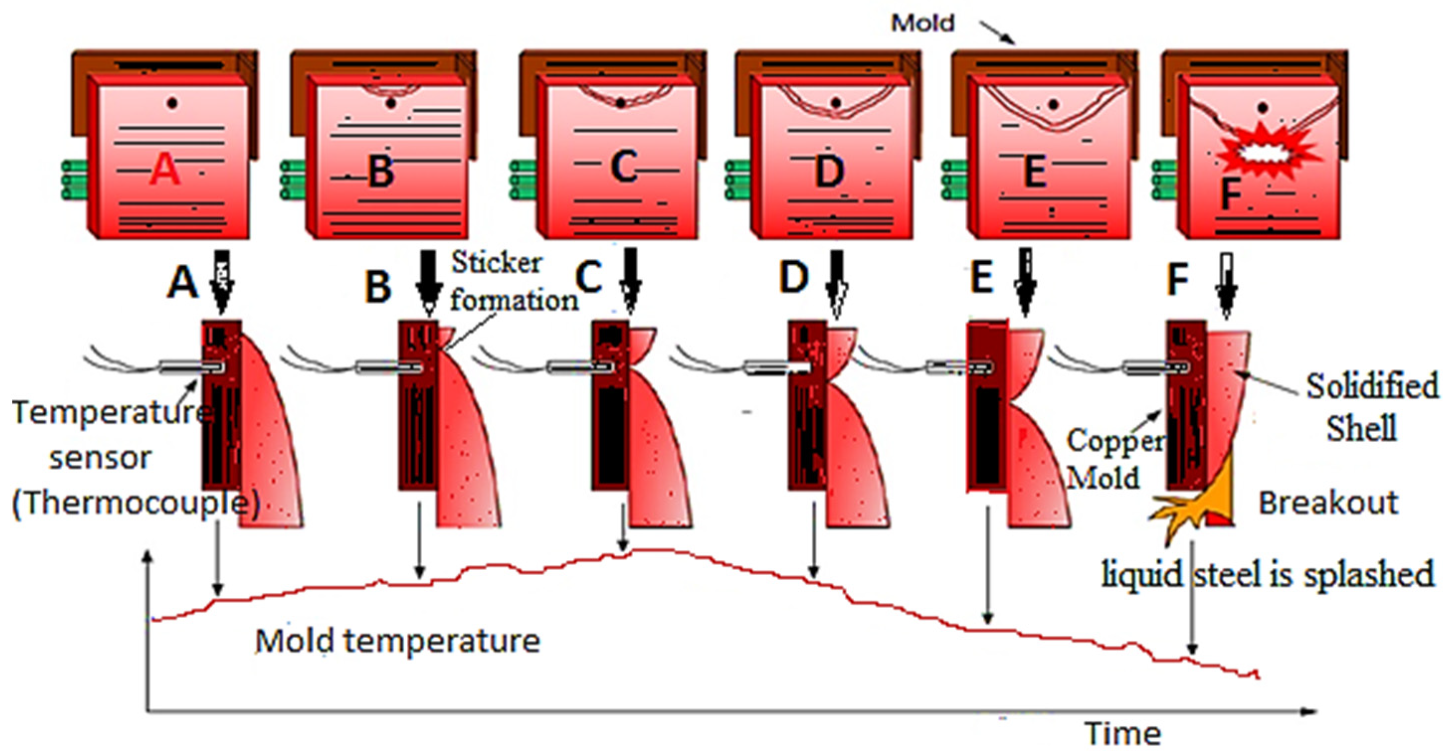
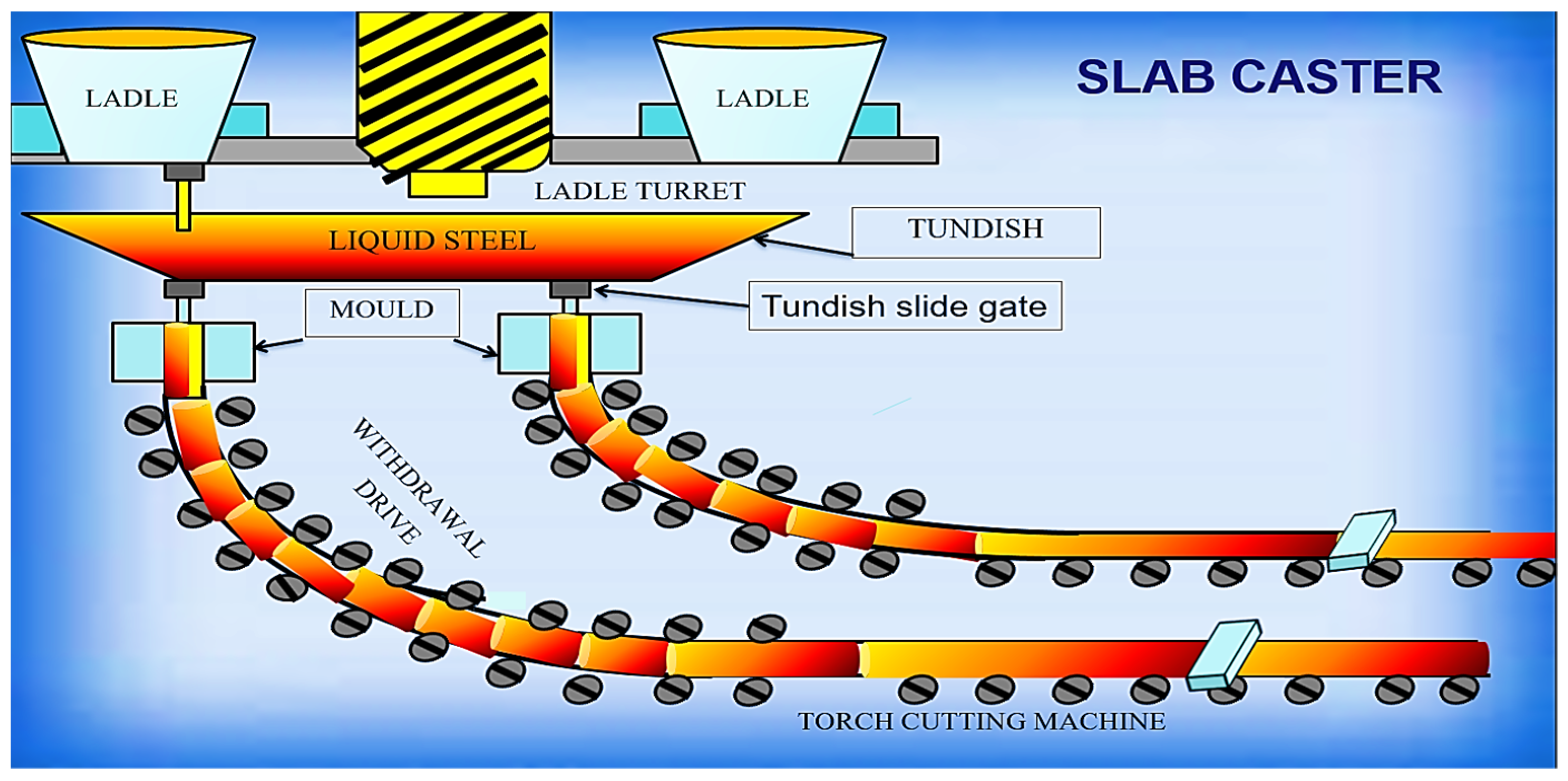
2. Process Description
3. Methodology
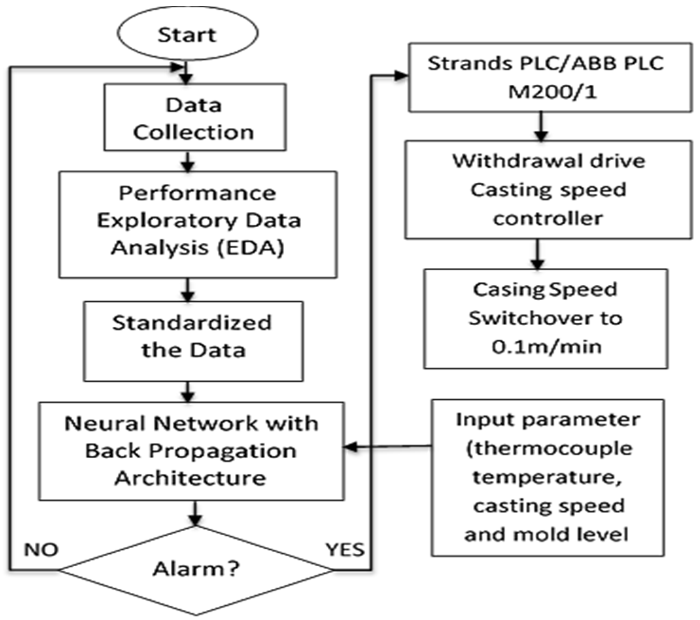
3.1. Design Flow Chart of Breakout Prediction Model
3.2. Exploratory Data Analysis (EDA)
3.2.1. Correlation Matrix
Calculation of the Correlation Coefficient
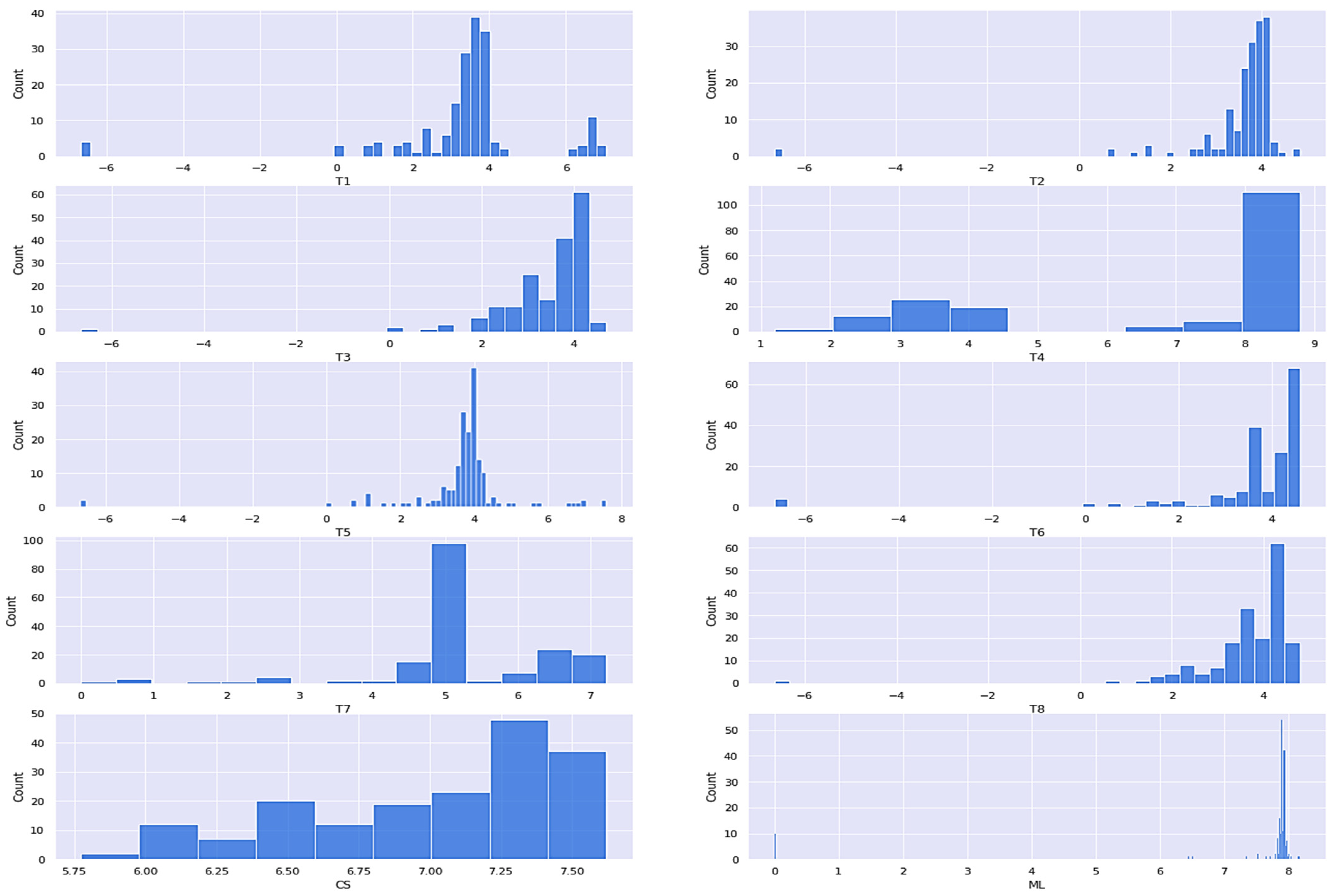
3.2.2. Histogram
3.3. Data Pre-Processing
3.3.1. Train Test Split
3.3.2. Standardizing the Data
3.4. Neural Network Architecture
Hidden and Output Layers and Activation Function
3.5. Dropout and Batch-Normalization
3.6. Selection of Optimizer and Loss Function
4. Results and Discussions
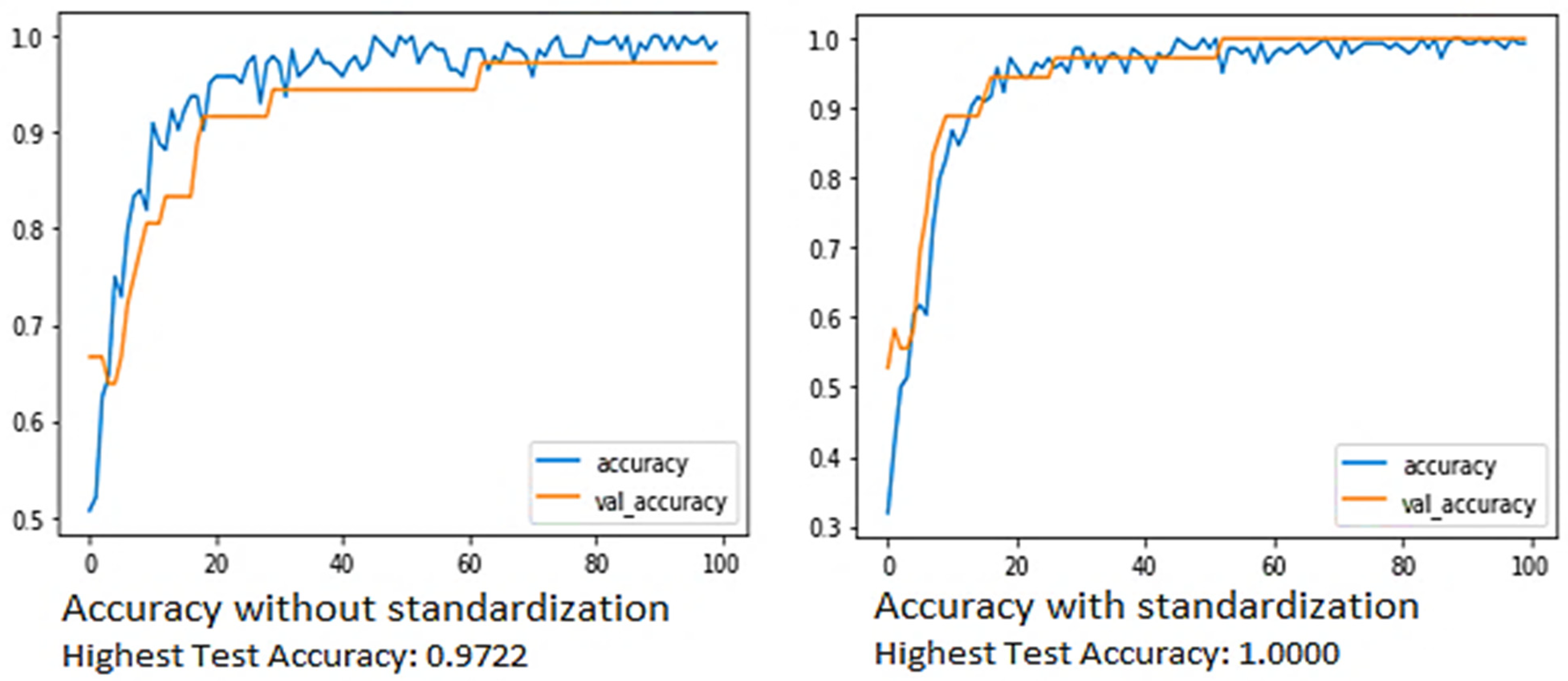
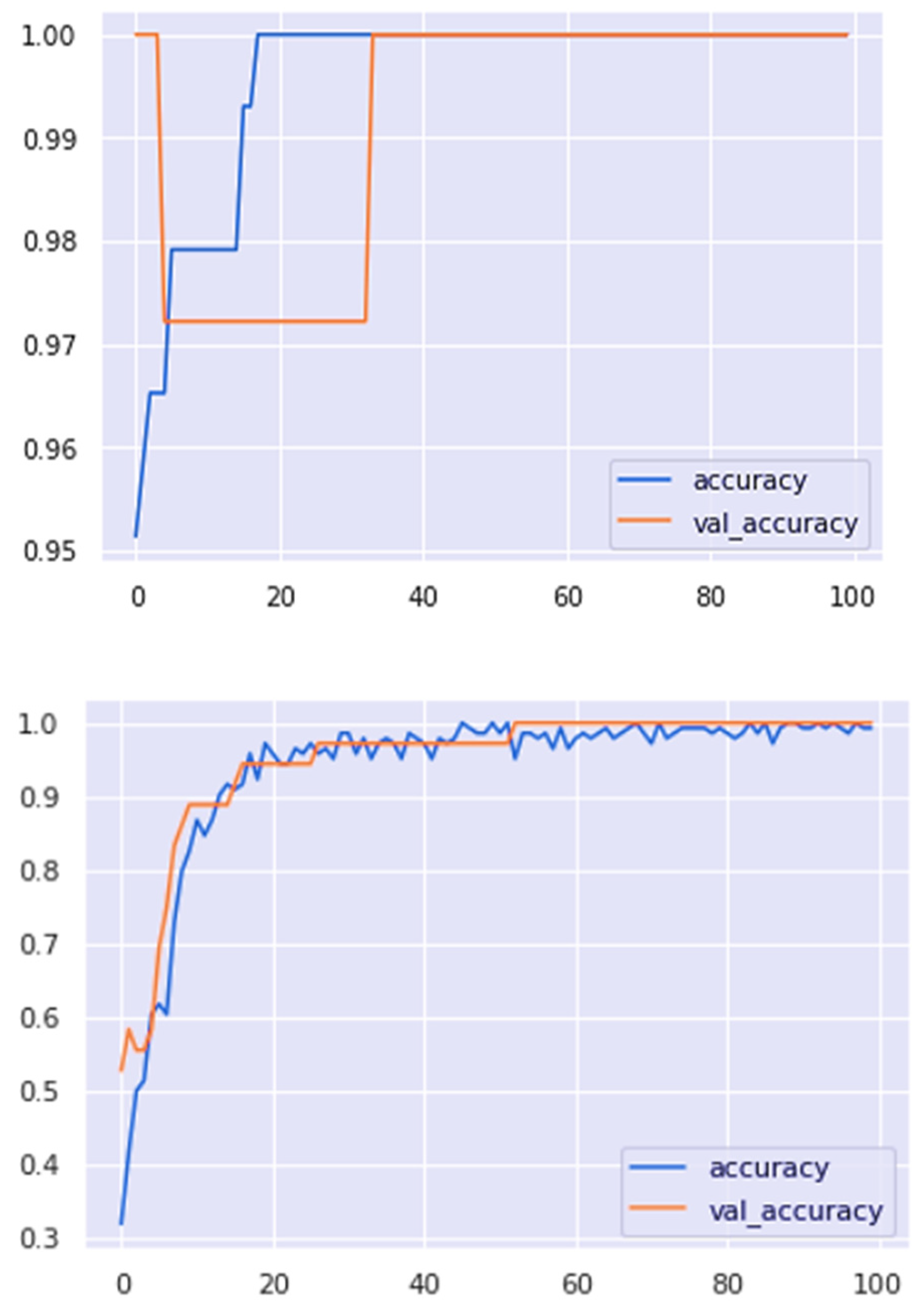
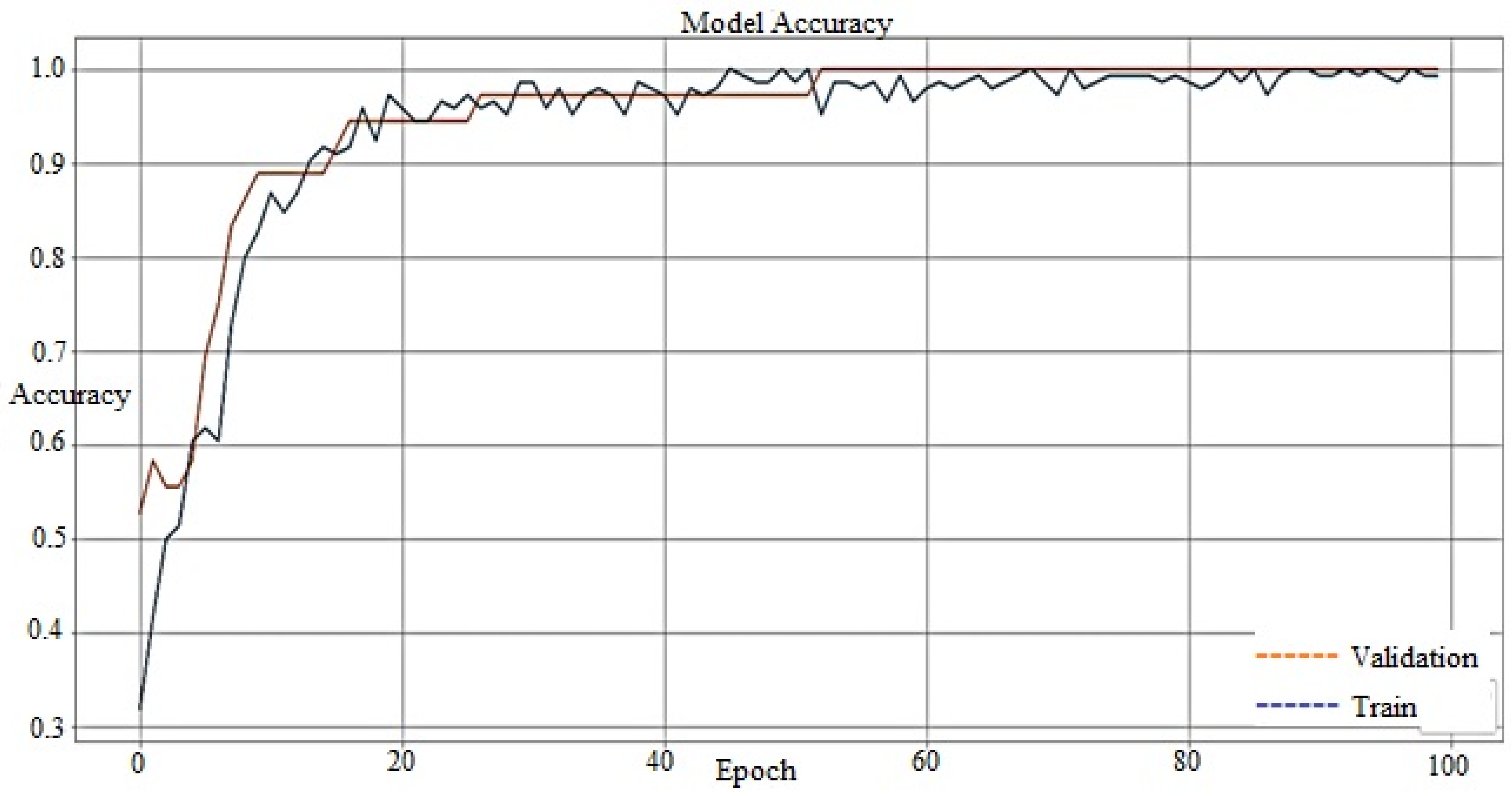
4.1. Accuracy Curve
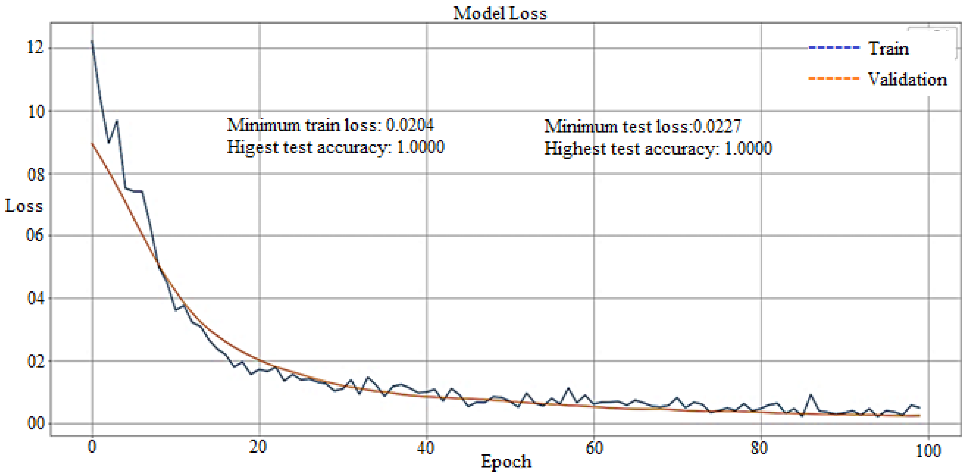
4.2. Loss Curve
4.3. Representative Field Application-Based Validation Test
5. Conclusions
6. Future Outlook: Development of a Framework for Automatic Reduction of Casting Speed
Author Contributions
Funding
Institutional Review Board Statement
Informed Consent Statement
Data Availability Statement
Conflicts of Interest
References
- Pan, E.; Ye, L.; Shi, J.; Chang, T.-S. On-line bleeds detection in continuous casting processes using engineering-driven rule-based algorithm. J. Manuf. Sci. Eng. 2009, 131, 061008. [Google Scholar] [CrossRef]
- Hore, S.; Das, S.K.; Humane, M.M.; Peethala, A.K. Neural Network Modelling to Characterize Steel Continuous Casting Process Parameters and Prediction of Casting Defects. Trans. Indian Inst. Met. 2019, 72, 3015–3025. [Google Scholar] [CrossRef]
- Louhenkilpi, S. Continuous casting of steel. In Treatise on Process Metallurgy; Elsevier: Amsterdam, The Netherlands, 2014; pp. 373–434. [Google Scholar]
- Qian, H.; He, F.; Xie, X.; Zhu, Z.; Zhang, L.; Zhang, L.; Shi, J. Recovery mechanism of the sticking-type breakout during continuous casting of steel. Ironmak. Steelmak. 2019, 46, 259–268. [Google Scholar] [CrossRef]
- Wang, W.; Zhu, C.; Zhou, L. Initial solidification and its related heat transfer phenomena in the continuous casting mold. Steel Res. Int. 2017, 88, 1600488. [Google Scholar] [CrossRef]
- Pereira, R.P.D.A.; de Almeida, G.M.; Salles, J.L.F.; Cuadros, M.A.D.S.L.; Valadão, C.T.; de Freitas, R.O.; Bastos-Filho, T. A Model-Based Predictive Controller of the Level of Steel in the Mold with Disturbances Using a Repetitive Structure. Metals 2021, 11, 1458. [Google Scholar] [CrossRef]
- Cho, S.-M.; Thomas, B.G. Electromagnetic forces in continuous casting of steel slabs. Metals 2019, 9, 471. [Google Scholar] [CrossRef] [Green Version]
- He, F.; Zhang, L. Mold breakout prediction in slab continuous casting based on combined method of GA-BP neural network and logic rules. Int. J. Adv. Manuf. Technol. 2018, 95. [Google Scholar] [CrossRef]
- Duan, H.; Wang, X.; Bai, Y.; Yao, M.; Liu, Y.; Guo, Q. Modeling of breakout prediction approach integrating feature dimension reduction with K-means clustering for slab continuous casting. Int. J. Adv. Manuf. Technol. 2020, 109, 2707–2718. [Google Scholar] [CrossRef]
- He, F.; Zhou, L. Formation Mechanism and Influence Factors of the Sticker between Solidified Shell and Mold in Continuous Casting of Steel. High Temp. Mater. Process. 2019, 38, 192–198. [Google Scholar] [CrossRef]
- Salah, B.; Zoheir, M.; Slimane, Z.; Jurgen, B. Inferential sensor-based adaptive principal components analysis of mold bath level for breakout defect detection and evaluation in continuous casting. Appl. Soft Comput. 2015, 34, 120–128. [Google Scholar] [CrossRef]
- Li, W.; Li, Y.; Zhang, Y. Study of mold breakout prediction technique in continuous casting production. In Proceedings of the 2010 3rd International Conference on Biomedical Engineering and Informatics, Yantai, China, 16–18 October 2010; Volume 7, pp. 2966–2970. [Google Scholar]
- Luk’Yanov, S.I.; Suspitsyn, E.S.; Krasilnikov, S.S.; Shvidchenko, D.V. Intelligent system for prediction of liquid metal breakouts under a mold of slab continuous casting machines. Int. J. Adv. Manuf. Technol. 2015, 79, 1861–1868. [Google Scholar] [CrossRef]
- He, F.; Zhou, L.; Deng, Z.-H. Novel mold breakout prediction and control technology in slab continuous casting. J. Process Control 2015, 29, 1–10. [Google Scholar] [CrossRef]
- He, F.; He, D.F.; Deng, Z.H.; Xu, A.J.; Tian, N. Development and application of mold breakout prediction system with online thermal map for steel continuous casting. Ironmak. Steelmak. 2015, 42, 194–208. [Google Scholar] [CrossRef] [Green Version]
- Watzinger, J.; Pesek, A.; Huebner, N.; Pillwax, M.; Lang, O. MoldExpert–operational experience and future development. Ironmak. Steelmak. 2005, 32, 208–212. [Google Scholar] [CrossRef]
- Qin, X.; Zhu, C.F.; Yin, Y.R.; Dong, X.R. Forecasting of molten steel breakouts for the slab continuous casters with hydraulic servo oscillation systems. Iron Steel Gangtie 2010, 45, 97–100. [Google Scholar]
- Qin, X.; Zhu, C.; Zheng, L. Study of the forecasting of molten steel breakouts based on the frictional force between mold and slab shell. In Proceedings of the 2010 International Conference on Mechanic Automation and Control Engineering, Wuhan, China, 26–28 June 2010; pp. 2593–2596. [Google Scholar]
- Bhattacharya, A.K.; Srinivas, P.S.; Chithra, K.; Jatla, S.V.; Das, J. Recognition of fault signature patterns using fuzzy logic for prevention of breakdowns in steel continuous casting process. In International Conference on Pattern Recognition and Machine Intelligence; Springer: Berlin/Heidelberg, Germany, 2005; pp. 318–324. [Google Scholar]
- Liu, Y.; Wang, X.; Du, F.; Yao, M.; Gao, Y.; Wang, F.; Wang, J. Computer vision detection of mold breakout in slab continuous casting using an optimized neural network. Int. J. Adv. Manuf. Technol. 2017, 88, 557–564. [Google Scholar] [CrossRef]
- Cheng, J.; Cai, Z.-Z.; Tao, N.-B.; Yang, J.-L.; Zhu, M.-Y. Molten steel breakout prediction based on genetic algorithm and BP neural network in continuous casting process. In Proceedings of the 31st Chinese Control Conference, Hefei, China, 25–27 July 2012; pp. 3402–3406. [Google Scholar]
- Zhang, B.-G.; Li, Q.; Wang, G.; Gao, Y. Breakout prediction based on BP neural network of LM algorithm in continuous casting process. In Proceedings of the 2010 International Conference on Measuring Technology and Mechatronics Automation, Changsha, China, 13–14 March 2010; Volume 1, pp. 765–768. [Google Scholar]
- Xu, Z.; Ma, L.; Zhang, Y.; Qin, X.; Cui, Y. Study on neural network breakout prediction system based on temperature unit input. In Proceedings of the 2010 International Conference on Measuring Technology and Mechatronics Automation, Changsha, China, 13–14 March 2010; Volume 3, pp. 612–615. [Google Scholar]
- Duan, H.; Wang, X.; Bai, Y.; Yao, M.; Guo, Q. Integrated approach to density-based spatial clustering of applications with noise and dynamic time warping for breakout prediction in slab continuous casting. Metall. Mater. Trans. B 2019, 50, 2343–2353. [Google Scholar] [CrossRef]
- Qin, X.; Zhu, C.-F.; Zheng, L.-W.; Yin, Y.-R. Molten steel breakout prediction based on thermal friction measurement. J. Iron Steel Res. Int. 2011, 18, 24–35. [Google Scholar] [CrossRef]
- Ren, T.; Shi, X.; Li, D.; Jin, X.; Wu, Y.; Sun, W. Research on breakout prediction system based on multilevel neural network. In Proceedings of the 2010 International Conference on Electrical and Control Engineering, Wuhan, China, 25–27 June 2010; pp. 1652–1655. [Google Scholar]
- Liu, K.; Peng, L.; Yang, Q. The algorithm and application of quantum wavelet neural networks. In Proceedings of the 2010 Chinese Control and Decision Conference, Xuzhou, China, 26–28 May 2010; pp. 2941–2945. [Google Scholar]
- Faizullin, A.; Zymbler, M.; Lieftucht, D.; Fanghanel, F. Use of deep learning for sticker detection during continuous casting. In Proceedings of the 2018 Global Smart Industry Conference (GloSIC), Chelyabinsk, Russia, 13–15 November 2018; pp. 1–6. [Google Scholar]
- Qing, T.; Wang, J.-W.; Xue, J.-S. Research for breakout prediction system based on support vector regression. In Proceedings of the 2012 IEEE Symposium on Robotics and Applications (ISRA), Kuala Lumpur, Malaysia, 3–5 June 2012; pp. 188–190. [Google Scholar]
- Duan, H.; Wang, X.; Bai, Y.; Yao, M.; Guo, Q. Application of k-means clustering for temperature timing characteristics in breakout prediction during continuous casting. Int. J. Adv. Manuf. Technol. 2020, 106, 4777–4787. [Google Scholar] [CrossRef]
- Liu, G.; Lu, H.; Li, B.; Ji, C.; Zhang, J.; Liu, Q.; Lei, Z. Influence of M-EMS on Fluid Flow and Initial Solidification in Slab Continuous Casting. Materials 2021, 14, 3681. [Google Scholar] [CrossRef]
- Yang, J.; Chen, D.; Qin, F.; Long, M.; Duan, H. Melting and Flowing Behavior of Mold Flux in a Continuous Casting Billet Mold for Ultra-High Speed. Metals 2020, 10, 1165. [Google Scholar] [CrossRef]
- Lei, Z.; Su, W. Mold level predict of continuous casting using hybrid EMD-SVR-GA algorithm. Processes 2019, 7, 177. [Google Scholar] [CrossRef] [Green Version]
- Su, W.; Lei, Z.; Yang, L.; Hu, Q. Mold-level prediction for continuous casting using VMD–SVR. Metals 2019, 9, 458. [Google Scholar] [CrossRef] [Green Version]
- Wang, Y.; Yang, S.; Wang, F.; Li, J. Optimization on Reducing Slag Entrapment in 150 × 1270 mm Slab Continuous Casting Mold. Materials 2019, 12, 1774. [Google Scholar] [CrossRef] [Green Version]
- Krajewski, W.; Miani, S.; Morassutti, A.C.; Viaro, U. Switching policies for mold level control in continuous casting plants. IEEE Trans. Control Syst. Technol. 2010, 19, 1493–1503. [Google Scholar] [CrossRef]
- Li, C.; Thomas, B.G. Ideal taper prediction for billet casting. In ISSTech-Conference Proceedings; Iron and Steel Society: Warrendale, PA, USA, 2003; pp. 685–700. [Google Scholar]
- Zhu, L.-G.; Kumar, R.V. Modelling of steel shrinkage and optimisation of mold taper for high-speed continuous casting. Ironmak. Steelmak. 2007, 34, 76–82. [Google Scholar] [CrossRef]
- Yang, H.; Lopez, P.E.R.; Vasallo, D.M. New Concepts for Prediction of Friction, Taper, and Evaluation of Powder Performance with an Advanced 3D Numerical Model for Continuous Casting of Steel Billets. Metall. Mater. Trans. B 2021, 52, 2760–2785. [Google Scholar] [CrossRef]
- Niu, Z.; Cai, Z.; Zhu, M. Dynamic distributions of mold flux and air gap in slab continuous casting mold. ISIJ Int. 2019, 59, 283–292. [Google Scholar] [CrossRef] [Green Version]
- Florio, B.J.; Vynnycky, M.; Mitchell, S.L.; O’Brien, S.B.G. On the interactive effects of mold taper and superheat on air gaps in continuous casting. Acta Mech. 2017, 228, 233–254. [Google Scholar] [CrossRef]
- Ratner, B. The correlation coefficient: Its values range between +1/−1, or do they? J. Target. Meas. Anal. Mark. 2009, 17, 139–142. [Google Scholar] [CrossRef] [Green Version]
- Raymaekers, J.; Rousseeuw, P.J. Transforming variables to central normality. Mach. Learn. 2021, 0, 1–23. [Google Scholar] [CrossRef]
- Srivastava, N.; Hinton, G.; Krizhevsky, A.; Sutskever, I.; Salakhutdinov, R. Dropout: A simple way to prevent neural networks from overfitting. J. Mach. Learn. Res. 2014, 15, 1929–1958. [Google Scholar]
- Ioffe, S.; Szegedy, C. Batch normalization: Accelerating deep network training by reducing internal covariate shift. In Proceedings of the 32nd International Conference on Machine Learning, Lille, France, 7–9 July 2015; pp. 448–456. [Google Scholar]
- Kingma, D.P.; Ba, J. Adam: A method for stochastic optimization. arXiv 2014, arXiv:1412.6980. [Google Scholar]
- Królczyk, G.; Legutko, S.; Królczyk, J.; Tama, E. Materials flow analysis in the production process-case study. In Applied Mechanics and Materials; Trans Tech Publications Ltd.: Freienbach, Switzerland, 2014; Volume 474, pp. 97–102. [Google Scholar]
- Mia, M.; Gupta, M.K.; Singh, G.; Królczyk, G.; Pimenov, D.Y. An approach to cleaner production for machining hardened steel using different cooling-lubrication conditions. J. Clean. Prod. 2018, 187, 1069–1081. [Google Scholar] [CrossRef]
- Ranjan, J.; Patra, K.; Szalay, T.; Mia, M.; Gupta, M.K.; Song, Q.; Krolczyk, G.; Chudy, R.; Pashnyov, V.A.; Pimenov, D.Y. Artificial intelligence-based hole quality prediction in micro-drilling using multiple sensors. Sensors 2020, 20, 885. [Google Scholar] [CrossRef] [Green Version]
- Singh, G.; Sharma, V.S.; Gupta, M.K.; Nguyen, T.T.; Królczyk, G.M.; Pimenov, D.Y. Parametric optimization of multi-phase MQL turning of AISI 1045 for improved surface quality and productivity. J. Prod. Syst. Manuf. Sci. 2021, 2, 5–16. [Google Scholar]
- Liu, Y.; Xu, Z.; Wang, X.; Zhang, D. Space–time characteristics of true and false sticker breakouts in mold during continuous casting. Ironmak. Steelmak. 2021, 48, 901–908. [Google Scholar] [CrossRef]


| Particular | Value |
|---|---|
| Number of breakouts | 23.6 per year |
| After the breakout, an average of 3 to 4 h is required to restart the Caster. Average delay due to breakout = (4 × 23.6) = 94.4 h/year | |
| The average weight of liquid steel loss | 3 ton per breakout |
| Total liquid steel loss | 3 × 23.6 = 70.80 tons per year |
| Cost of one ton of liquid steel | 44,000 INR |
| Loss of liquid steel per year | 31.15 million INR/year |
| Input Parameters | Maximum Value | Minimum Value |
|---|---|---|
| Thermocouple’s temperature (T1, T2 … T8) | 250 °C | 50 °C |
| Casting speed | 0.70 m/min | 0.50 m/min |
| Speed setpoint | 00 m/min | 00 m/min |
| Mold level | Always greater than or equal to 20% | |
| Default upper thermocouple’s temperature always shows = 300 °C | ||
| Default lower thermocouple’s temperature always shows = 0 °C | ||
| Output parameter: | Output of this model is either ‘1’ for breakout and generate alarm or ‘0’ for no breakout and not generate any alarm | |
| Breakout S.No. | Date and Time | Heat Number | Strand Number | Slab Size (mm) | Heat of Sequence | Ladle Number | Steel Grade | Casting Speed (m/min) | Mold Level (%) |
|---|---|---|---|---|---|---|---|---|---|
| T1(°C) | T2(°C) | T3(°C) | T4(°C) | T5(°C) | T6(°C) | T7(°C) | T8(°C) | ||
| 01 | 11 May 2021 06:30:30 | 53,969 | 02 | 1045 | 1st | 14 | CR2B | 0.77 | 0 |
| 186 | 8 | 146 | 9 | 10 | 76 | −5 | 6 | ||
| 02 | 31 May 2021 04:10:02 | 54,335 | 02 | 1090 | 1st | 21 | GR-II | 0.90 | 0 |
| 188 | 12 | 132 | 3 | −2 | 95 | 2 | 2 | ||
| 03 | 09 September 2021 03:17:56 | 57,263 | 04 | 1045 | 5th | 13 | GR-II | 1.22 | 60 |
| 13 | 130 | 20 | 14 | −11 | 60 | 22 | 10 | ||
| 04 | 27 September 2021 22:50:31 | 57,803 | 4 | 1090 | 4th | 9 | CR | 1.01 | 62 |
| 15 | 6 | 15 | 10 | 21 | 46 | 4 | −11 | ||
| 05 | 07 October 2021 06:17:59 | 58,132 | 1 & 2 | 1470/1320 | 8th | 18 | GR-II Patton | 1.32 | 64 |
| 178 | 32 | 178 | 14 | −15 | 169 | 31 | 30 | ||
| 06 | 28 October 2021 23:17:38 | 58,898 | 2 | 1045 | 8th | 23 | CR2 | 1.09 | 54 |
| 194 | 0 | 125 | −12 | −8 | 125 | −3 | -3 | ||
| 07 | 31 October 2021 06:30:30 | 58,974 | 4 | 1320 | 6th | 17 | GR-I | 1.02 | 60 |
| 4 | 10 | −13 | 5 | 4 | 210 | −12 | 5 | ||
| 08 | 09 September 2021 20:47:33 | 57,263 | 4 | 1045 | 5th | 13 | GR-II | 0.78 | 0 |
| 2 | −1 | 1 | 0 | −6 | 1 | −13 | 7 | ||
| 09 | 27 September 2021 02:44:48 | 57,803 | 4 | 1090 | 4th | 9 | CR | 0.50 | 1 |
| 54 | −14 | 55 | −13 | −17 | 63 | −16 | −18 | ||
| 10 | 07 October 2021 03:47:49 | 58,132 | 1 & 2 | 1470/1320 | 8th | 18 | GR-II Patton | 0.38 | 0 |
| −38 | −6 | 93 | −5 | −9 | 49 | −4 | −5 | ||
| 11 | 28 October 2021 12:49:60 | 58,898 | 2 | 1045 | 8th | 23 | CR2 | 1.08 | 39 |
| −1 | −1 | −5 | −17 | −15 | 208 | −12 | 1 | ||
| 12 | 31 October 2021 20:55:03 | 58,974 | 4 | 1320 | 6th | 17 | GR-I | 1.22 | 60 |
| 19 | 133 | 21 | 10 | −11 | 51 | 18 | 14 | ||
| 13 | 03 November 2021 13:51:14 | 59,060 | 3 | 1320 | 5th | 25 | GR-II | 0.77 | 0 |
| 189 | 8 | 146 | 9 | 10 | 79 | −5 | 6 |
| Parameters | New Model | Actual BOPS |
|---|---|---|
| Total number of heats | 5299 | 5299 |
| Total number of true breakout alarms | 13 | 13 |
| Total number of missed breakout alarms | 00 | 13 |
| Total numbers of false breakout alarms | 06 | 21 |
| Frequency of false alarms (%) | 0.113 | 0.396 |
| Breakout detection ratio (%) | 100 | 50 |
| Breakout prediction accuracy ratio (%) | 100 | 27 |
| Authors | Breakout Detection Ratio | Breakout Prediction Accuracy Ratio | Frequency of False Alarm |
|---|---|---|---|
| New model | 100% | 100% | 0.113 |
| Liu, Yu, et al. [51] | 98.73% | 98.7% | 0.126 |
| He, Fei, et al. [15] | 100% | 78.26% | 0.150 |
| He, Fei, et al. [8] | 100% | 82.60% | 0.1365 |
Publisher’s Note: MDPI stays neutral with regard to jurisdictional claims in published maps and institutional affiliations. |
© 2022 by the authors. Licensee MDPI, Basel, Switzerland. This article is an open access article distributed under the terms and conditions of the Creative Commons Attribution (CC BY) license (https://creativecommons.org/licenses/by/4.0/).
Share and Cite
Ansari, M.O.; Chattopadhyaya, S.; Ghose, J.; Sharma, S.; Kozak, D.; Li, C.; Wojciechowski, S.; Dwivedi, S.P.; Kilinc, H.C.; Królczyk, J.B.; et al. Productivity Enhancement by Prediction of Liquid Steel Breakout during Continuous Casting Process in Manufacturing of Steel Slabs in Steel Plant Using Artificial Neural Network with Backpropagation Algorithms. Materials 2022, 15, 670. https://0-doi-org.brum.beds.ac.uk/10.3390/ma15020670
Ansari MO, Chattopadhyaya S, Ghose J, Sharma S, Kozak D, Li C, Wojciechowski S, Dwivedi SP, Kilinc HC, Królczyk JB, et al. Productivity Enhancement by Prediction of Liquid Steel Breakout during Continuous Casting Process in Manufacturing of Steel Slabs in Steel Plant Using Artificial Neural Network with Backpropagation Algorithms. Materials. 2022; 15(2):670. https://0-doi-org.brum.beds.ac.uk/10.3390/ma15020670
Chicago/Turabian StyleAnsari, Md Obaidullah, Somnath Chattopadhyaya, Joyjeet Ghose, Shubham Sharma, Drazan Kozak, Changhe Li, Szymon Wojciechowski, Shashi Prakash Dwivedi, Huseyin Cagan Kilinc, Jolanta B. Królczyk, and et al. 2022. "Productivity Enhancement by Prediction of Liquid Steel Breakout during Continuous Casting Process in Manufacturing of Steel Slabs in Steel Plant Using Artificial Neural Network with Backpropagation Algorithms" Materials 15, no. 2: 670. https://0-doi-org.brum.beds.ac.uk/10.3390/ma15020670