A Nonlinear Control of Linear Slider Considering Position Dependence of Interlinkage Flux ^†

Abstract

Linear sliders are linear actuators using linear motors. It is used in many applications, such as factory lines and linear motor cars. In recent years, the demand for smaller semiconductor devices has been increasing due to the proliferation of smartphones. High-precision positioning of linear motors is needed because manufacturing semiconductor devices uses the stage with linear motors. However, linear motors have nonlinearity due to the position dependence of interlinkage flux. It affects precise positioning. In this study, the nonlinear characteristics due to the position dependence of the flux are expressed as a mathematical model by using a distributed constant magnetic circuit. A method compensating it using an operator-based feedback controller with the obtained mathematical model is proposed. The effectiveness of the proposed method is confirmed by simulating and experimenting with the reference following disturbance elimination.

1. Introduction

A linear slider is a linear actuator using a linear motor, and a linear motor is a motor that can move linearly directly. Since it does not need a linear motion mechanism, such as a ball screw, it has advantages, such as low friction and long stroke operation, and it is used in many applications such as machine tools in factory lines and linear motor cars. In recent years, the demand for smaller semiconductor devices has been increasing due to the proliferation of smartphones. The stages using linear motors are widely used in the manufacture of semiconductor devices. Therefore, to make smaller semiconductor devices, more high-precision position control of the linear motor is needed. However, linear motors contain nonlinearity due to the position dependence of interlinkage flux, which makes them more difficult to control than rotary motors.

In Miyakawa’s study, the misalignment of the center of gravity caused by the sensor is compensated for by building a motion model at the center of gravity and using an observer to estimate the center of gravity’s position from the observed values [1]. In Takahashi’s study, a compactly structured, magnetic levitation nano-positioning stage is developed, and a 6-degrees-of-freedom controller is used to control the positioning of the stage [2]. In Mitsui’s study, the detent force of the permanent magnet linear synchronous motor was eliminated without compromising thrust by adjusting the position of the mover magnet [3]. In Manabe’s study, a sensor to measure the jerk, which is the time derivative of acceleration, was developed, and it was used to control the inertia of the linear motor by providing feedback from the acceleration obtained by integrating the jerk [4]. In Nakamura’s study, the learning accuracy of the inverse system of a linear slider was improved by using references with multiple frequencies [5]. In Shao’s study, the parameter variations and disturbances of the linear motor are compensated for using RTSMC with ADO [6]. In Zhang’s study, a fast NTSMC designed by using ELM is proposed. It controls the position of the linear motor in simulations [7]. In Shirani’s study, a fluctuation of the pneumatic anti-vibration table caused by air pressure supply is eliminated by using a voice coil motor and its controller [8]. In Liu’s study, three differential, adaptive controllers are proposed to control PMLSM [9].

In this study, a feedback controller based on operator theory is used to compensate for nonlinearity and ensure stability. Operator theory is a control method to analyze a control system by representing the system dynamics with nonlinear maps that represent their input and output characteristics (called operators). This expression enables the BIBO stability of a nonlinear system to be analyzed easily, unlike transfer function and state-space expression. Moreover, it can use the coprime factorization technic via robust control theory. Therefore, the stability of a closed-loop system based on operator theory is ensured by the right coprime factorization of the system. It can be used for a variety of plants because this method does not require a specific form of nonlinearity, such as quadratic, trigonometric function, etc., for a plant. However, in this theory, it is difficult to ensure the performance tracking to the reference value. Therefore, in each study of operator theory, tracking controllers are also proposed in addition to the stability guarantee [10,11,12,13,14,15,16,17,18,19,20,21,22,23].

In a previous study, a linear dynamic model was used to control a linear motor, which was designed and analyzed using a transfer function representation with Laplace transform. A transfer function-based disturbance observer without using a differentiator was proposed to compensate for disturbances and uncertainties. It was confirmed that the controller allowed the output to follow the reference value [24,25]. However, there are nonlinear elements that cannot be fully compensated for by the linear model and the disturbance observer, and these elements cause errors during position control.

In this study, we focus on the parameter variations of the linear motor depending on the stage position and propose a method to compensate for the parameter variation. Specifically, the flux interlinking the armature coil is represented by a distributed magnetic circuit based on the structure of the linear motor. A mathematical model is created by combining the characteristics obtained by analyzing the circuit with a general linear model. In addition, the nonlinearity is compensated for using operator-based robust right coprime factorization of the plant, and the tracking performance for reference is compensated by a 2-degrees-of-freedom (2-DOF) controller. Furthermore, a disturbance observer using the gradient descent method is added to eliminate the effect of disturbance.

The contents of this paper are as follows. First, the mathematical preparation of operator theory and nonlinear observer is shown in Section 2. Second, the experiment system used in this study and problem statement is introduced in Section 3. Third, the mathematical model of the linear motor is derived in Section 4. Fourth, the position controller for the linear motor is designed in Section 5. Fifth, the simulation and experimental results are presented in Section 6. Finally, the conclusion is given in Section 7.

2. Mathematical Preparation

This chapter describes the operator theory used to design the control system and defines and introduces the mathematical knowledge required for this theory.

2.1. Definition of Operator

In operator theory, vector space is used for designing a controller instead of a transfer function or state-space. The operator in this study is the map transforming from any input space into output space. Therefore, nonlinear characteristics of the plant are able to be expressed as the map related to the signal input to the output. In this study, the expression $Q:U\to Y$ is the mapping from input space U to output space Y in the time domain. Similarly, $y\left(t\right)=Q\left(u\right)\left(t\right)$ is the output $y\left(t\right)$ mapped from input $u\left(t\right)$ using operator Q.

2.2. Unimodular Operator

Let $\mathcal{S}\left(U_s,Y_s\right)$ be the set of stable operators that map from $U_s$ to $Y_s$. $\mathcal{U}\left(U,Y\right)$ is the subset of $\mathcal{S}\left(U_s,Y_s\right)$, and it satisfies (1).

$$\begin{array}{cc}\hfill \mathcal{U}\left(U,Y\right)=& \{M:M\in \mathcal{S}\left(U,Y\right),\hfill \\ \hfill & M\mathrm{is}\mathrm{invertible}\mathrm{with}{M}^{-1}\in \mathcal{S}\left(Y,U\right)\}\hfill \end{array}$$

(1)

where the operator $M\in \mathcal{U}$ is called the unimodular operator.

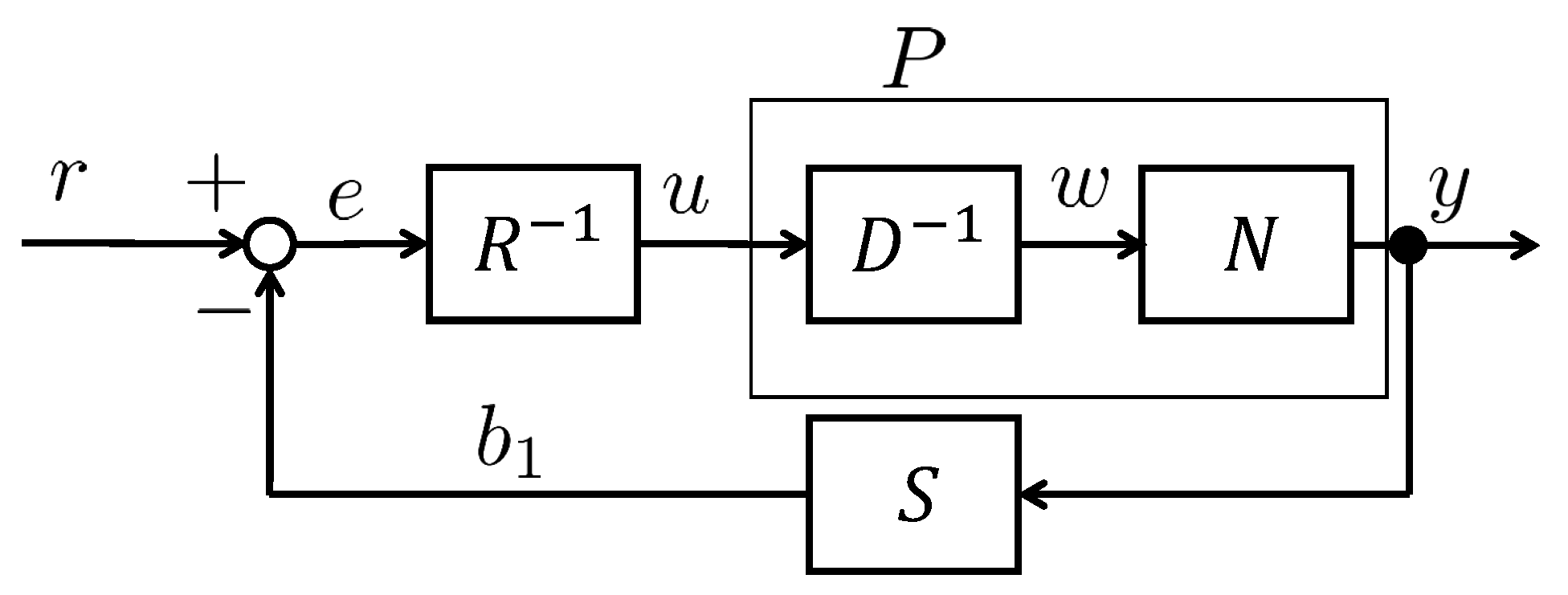
2.3. Operator-Based Feedback Controller

Analyzing the stability of the feedback controller is shown in Figure 1. Let $P:U\to Y:y\left(t\right)=P\left(u\right)\left(t\right)$ be a control plant operator. Where U and Y are the input and output signal spaces. They are two different extended linear spaces. In this case, plant P is

$$\begin{array}{c}\hfill P=N{D}^{-1}\end{array}$$

(2)

where $N:W\to Y$ is the stable operator, and $D:W\to U$ is the stable and invertible operator. If there exists a continuous quasi-state $w\left(t\right)\in W$ and extended linear space depending on plant P, then plant P is said to have a “Right Factorization” of N and D. Furthermore, P is said to have “Right Coprime Factorization” of N and D if operators N and D satisfy the following Bézout’s identity

$$\begin{array}{c}\hfill SN\left(w\right)\left(t\right)+RD\left(w\right)=M\left(w\right)\left(t\right),M\in \mathcal{U}\left(W,U\right)\end{array}$$

(3)

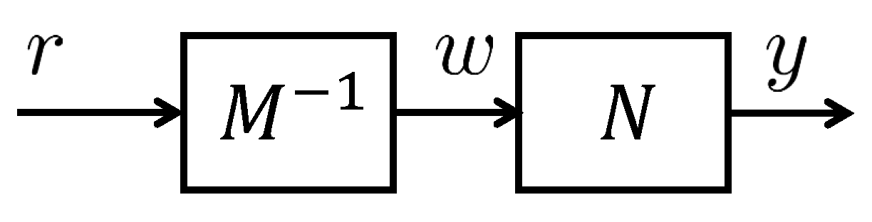
where $S:Y\to U$ is a stable operator, $R:U\to U$ is a stable and invertible operator, and $M:W\to U$ is a unimodular operator. The robust stability of P is ensured by operator-based feedback in Figure 1, and the response from $r\left(t\right)\in U$ to $w\left(t\right)$ is expressed by the operator $M^{-1}$ equivalently. Therefore, the response of the system is expressed as (4)

$$\begin{array}{c}\hfill y\left(t\right)=N{M}^{-1}\left(r\right)\left(t\right)\end{array}$$

(4)

The block diagram is shown in Figure 2.

2.4. Ensuring Robust Stability for Uncertainty

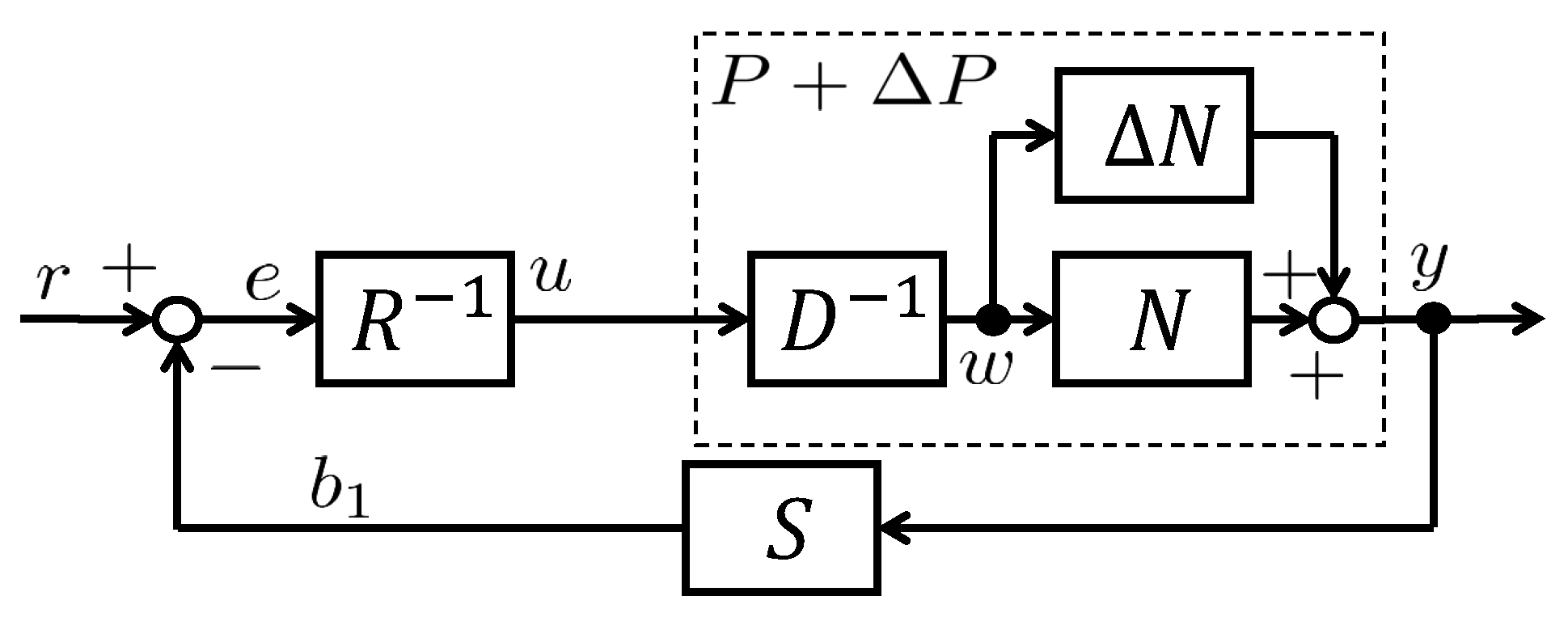
Actual plants have uncertainties that are not included in the mathematical model, such as parameter variations and disturbances. The controller’s stability does not prevent by unstable elements, which have uncertainty even if $D^{-1}$ includes all unstable elements of a nominal plant. Therefore, in this section, robust stability is ensured, which enables using all stabilized conditions.

The nonlinear feedback system, including uncertainty in a control plant, is shown in Figure 3. Let P be a nominal plant that does not include uncertainty. The actual plant, including uncertainty, is expressed by adding nominal plant P and uncertainty element $\Delta P$, such as $\tilde{P}=P+\Delta P$. The right factorization of the actual plant $\tilde{P}$ is

$$\begin{array}{c}\hfill \tilde{P}\left(u\right)\left(t\right)=\left(P+\Delta P\right)\left(u\right)\left(t\right)=(N+\Delta N)D^{-1}\left(u\right)\left(t\right)\end{array}$$

(5)

It is known that uncertainty $\Delta P$ is consolidated into an operator $\Delta N$. It is hard to derive $\Delta N$ by calculation and measurement. However, it is known that the output is bounded. To ensure the BIBO stability of the plant, including uncertainty, Beźout’s identity for $\tilde{P}$ is expressed (6).

$$\begin{array}{c}\hfill S(N+\Delta N)+RD=\tilde{M}\end{array}$$

(6)

If it is proved that $\tilde{M}$ is a unimodular operator, $\left(N+\Delta N\right)$ and D are coprimes, i.e., its stability is proved. $\tilde{M}$ from (3) and (6) is shown in (7)

$$\begin{array}{cc}\hfill \tilde{M}-M& =S\left(N+\Delta N\right)-SN\hfill \\ \hfill \tilde{M}& =\left[I+\left(S\left(N+\Delta N\right)-SN\right)M^{-1}\right]M\hfill \end{array}$$

(7)

An operator $\tilde{M}$ is clearly stable from (7) since it has only stable operators. Therefore, the stability of ${\tilde{M}}^{-1}$ is proven. ${\tilde{M}}^{-1}$ is expressed as

$$\begin{array}{cc}\hfill {\tilde{M}}^{-1}& =M^{-1}{\left[I+\left(S\left(N+\Delta N\right)-SN\right)M^{-1}\right]}^{-1}\hfill \end{array}$$

(8)

where $M^{-1}$ is a stable operator since it is a unimodular operator, and the other part indicates a feedback system with $\left(S\left(N+\Delta N\right)-SN\right)M^{-1}$ as an open-loop operator. Using the small-gain theorem, the stability of ${\tilde{M}}^{-1}$ is ensured if it satisfies (9). Then, $\tilde{M}$ is a unimodular operator, and the robust stability of the system is ensured.

$$\begin{array}{c}\hfill {∥(S(N+\Delta N)-SN)M^{-1}∥}_{Lip}<1\end{array}$$

(9)

2.5. Gradient Descent Method Based Nonlinear Observer

It is hard to estimate state variables in a nonlinear state-space (10) indicated using a general linear observer (11).

$$\begin{array}{cc}\hfill & \left\{\begin{array}{c}\dot{\mathit{x}}\left(t\right)=\mathit{f}(\mathit{x},u)\left(t\right)\hfill \\ y\left(t\right)=h\left(\mathit{x}\right)\left(t\right)\hfill \end{array}\right.\hfill \end{array}$$

(10)

$$\begin{array}{cc}\hfill & \dot{\widehat{\mathit{x}}}\left(t\right)=\mathit{A}\widehat{\mathit{x}}\left(t\right)+\mathit{b}u\left(t\right)+\mathit{l}\left(y\left(t\right)-\mathit{c}\widehat{\mathit{x}}\left(t\right)\right)\hfill \end{array}$$

(11)

A nonlinear observer is needed to estimate state variables. In this study, a nonlinear observer is used to estimate the gradient descent method [26,27]. This observer is expressed as (12). It uses evaluation function J and nonlinear state equation $\mathit{f}$ to estimate the state variables. Where $\mathit{H}$ is the coefficient for stabilization.

$$\begin{array}{c}\hfill \dot{\widehat{\mathit{x}}}\left(t\right)=\mathit{f}(\widehat{\mathit{x}},u)\left(t\right)-\frac{1}{2}\mathit{H}\left(t\right)\frac{\partial J(y,\widehat{\mathit{x}})}{\partial \widehat{\mathit{x}}}\left(t\right)\end{array}$$

(12)

where J is constructed as squares of estimation output error, i.e.,

$$\begin{array}{c}\hfill J(y,\widehat{\mathit{x}})\left(t\right)={\left(y\left(t\right)-h\left(\widehat{\mathit{x}}\right)\left(t\right)\right)}^2\end{array}$$

(13)

To substitute it into (14), the estimated states are

$$\begin{array}{c}\hfill \dot{\widehat{\mathit{x}}}\left(t\right)=\mathit{f}(\widehat{\mathit{x}},u)\left(t\right)+\mathit{H}\left(t\right)\frac{\partial h\left(\widehat{\mathit{x}}\right)}{\partial \widehat{\mathit{x}}}\left(t\right)\left(y\left(t\right)-h\left(\widehat{\mathit{x}}\right)\left(t\right)\right)\end{array}$$

(14)

Stabilizing

$\mathit{H}$ is designed to stabilize the observer in this section. Let $\mathit{e}$ be the estimation error, which is defined as follows

$$\begin{array}{c}\hfill \mathit{e}=\mathit{x}-\widehat{\mathit{x}}\end{array}$$

(15)

(16) is obtained to derive the state equation of it.

$$\begin{array}{c}\hfill \dot{\mathit{e}}\left(t\right)=\mathit{f}(\mathit{x},u)\left(t\right)-\mathit{f}(\widehat{\mathit{x}},u)\left(t\right)-\mathit{H}\left(t\right)\frac{\partial h\left(\widehat{\mathit{x}}\right)}{\partial \widehat{\mathit{x}}}\left(t\right)\left(y\left(t\right)-h\left(\widehat{\mathit{x}}\right)\left(t\right)\right)\end{array}$$

(16)

Assuming that the estimation error is near zero, (16) is expressed as (17) using the first approximation.

$$\begin{array}{c}\hfill \dot{\mathit{e}}\left(t\right)={\left.\left(\frac{\partial \mathit{f}(\mathit{x},u)}{\partial \widehat{\mathit{x}}}\left(t\right)-\mathit{H}\left(t\right){\frac{\partial h\left(\mathit{x}\right)}{\partial \widehat{\mathit{x}}}}^2\left(t\right)\right)\right|}_t\mathit{e}\left(t\right)\end{array}$$

(17)

If the Lyapunov function exists at $\mathit{e}=\mathbf{0}$ in Equation (17), it is asymptotically stable at $\mathit{e}=\mathbf{0}$. Therefore, (18) is created as a candidate for the Lyapunov function. Where $\mathit{P}$ is a positive definite symmetric matrix.

$$\begin{array}{c}\hfill V\left(\mathit{e}\right)={\mathit{e}}^T\mathit{Pe}\end{array}$$

(18)

Derivating it, the following equation is expressed

$$\begin{array}{cc}\hfill \dot{V}\left(\mathit{e}\right)& ={\mathit{e}}^T\mathit{P}\dot{\mathit{e}}+{\dot{\mathit{e}}}^T\mathit{P}\mathit{e}\hfill \\ \hfill & ={\mathit{e}}^T\left(\mathit{P}{\mathit{A}}_o\left(t\right)+{\mathit{A}}_o{\left(t\right)}^T\mathit{P}\right)\mathit{e}\hfill \\ \hfill {\mathit{A}}_o\left(t\right)& ={\left.\left(\frac{\partial \mathit{f}(\mathit{x},u)}{\partial \widehat{\mathit{x}}}\left(t\right)-\mathit{H}\left(t\right){\frac{\partial h\left(\mathit{x}\right)}{\partial \widehat{\mathit{x}}}}^2\left(t\right)\right)\right|}_t\hfill \end{array}$$

(19)

Therefore, the stability of this observer is ensured if the positive definite matrix $\mathit{Q}$ satisfying the Lyapunov Equation (20) exists.

$$\begin{array}{c}\hfill {\mathit{A}}_o{\left(t\right)}^T\mathit{P}+\mathit{P}{\mathit{A}}_o\left(t\right)=-\mathit{Q}\end{array}$$

(20)

3. Experimental System and Problem Statements

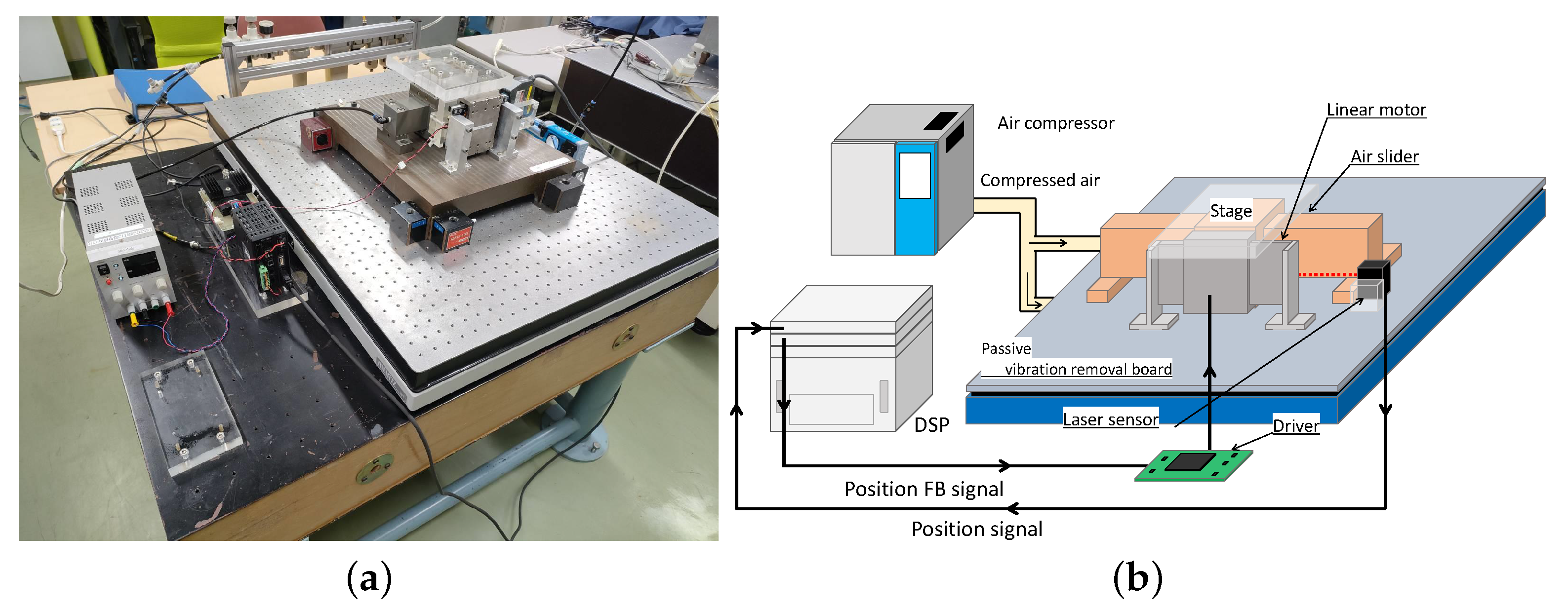
A picture of an experimental system is shown in Figure 4. The control plant is a linear stage constructed linear motor and air slider with bolts. An air slider works to eliminate the effect of friction when it receives compressed air from the air compressor. The stage is moved right and left by the flowing electric current from the linear motor. A laser displacement sensor installed on the side of the stage measures the position of the stage and sends the signal to the digital signal processor (DSP). When it is received by the DSP, the DSP calculates the signal from the sensor-based designed system. The signal calculated by the DSP is sent to the driver circuit for the linear motor. The circuit amplifies its current and sends it to the linear motor. Throughout the processes, the position of the stage is controlled to a reference value. A passive vibration removal board is installed under the stage. It works to remove vibration from the ground.

3.1. Voice Coil Motor

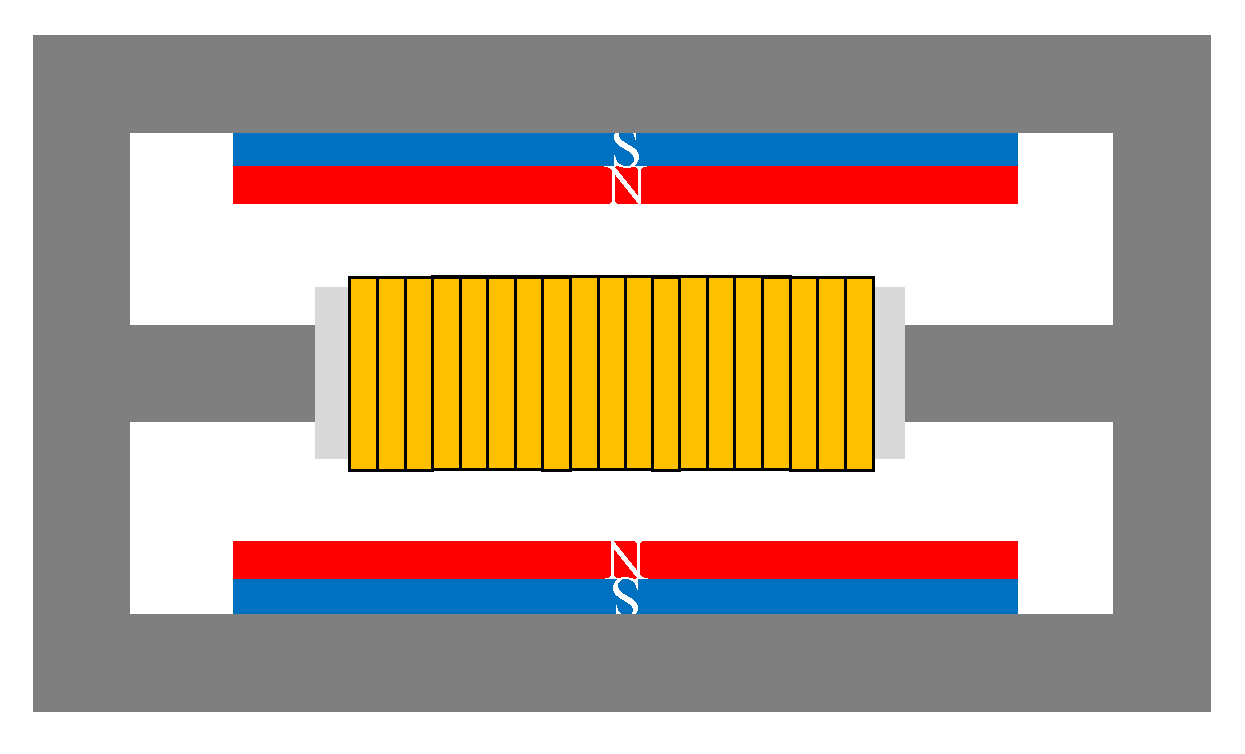
In this study, the voice coil motor (VCM) is one of the linear motors used to control the position of the stage. The structure of VCM is shown in Figure 5. It is known from the figure that VCM has only one pair of permanent magnets. It is a particularly distinctive element compared with a general linear motor. From the structure, it moves based on a principle similar to speakers. It has the disadvantage that it cannot make a long stroke. However, it has many advantages; its weight is very light, it has near-linear thrust, it can minimize easily, and more. Because of that, it is mainly used for autofocusing smartphone cameras.

3.2. Problem Statement

The purpose of this study is to control the position of the linear slider precisely. Specifically, a model of a linear motor considering the position dependence of interlinkage flux is proposed, and it is compensated by an operator-based nonlinear feedback controller.

4. Model of the Plant

4.1. Linear Model

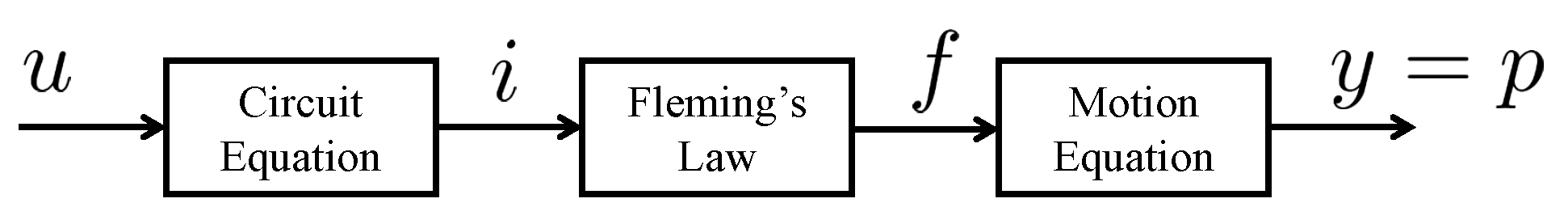
The signal of VCM is converted from voltage u to current i, force f, and finally, position p, which is shown in Figure 6. In this section, the equations of the blocks are expressed.

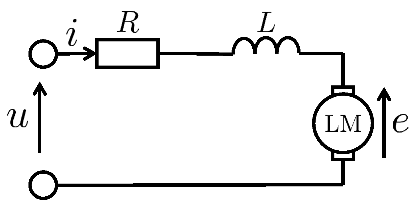
A circuit equation is the equation of the armature coil-equipped VCM. The armature coil is equivalently expressed as RL series circuit and back-emf due to interlinkage flux.

Therefore, it is expressed in Figure 7 by a circuit diagram and by differential Equation (21). Where v is the velocity of the stage.

$$\begin{array}{c}\hfill \frac{d}{dt}i\left(t\right)=-\frac{\mathsf{\Phi }}{L}v\left(t\right)-\frac{R}{L}i\left(t\right)+\frac{1}{L}u\left(t\right)\end{array}$$

(21)

The conversion from current i to force f is expressed as a linear combination of current in (22) since Fleming’s left-hand rule holds.

$$\begin{array}{c}\hfill f\left(t\right)=\mathsf{\Phi }i\left(t\right)\end{array}$$

(22)

A conversion from force f to position p is expressed as a second-order differential equation indicated by (23) considering the mass spring damper system.

$$\begin{array}{c}\hfill \frac{d^2}{d{t}^2}p\left(t\right)=-\frac{k}{m}p\left(t\right)-\frac{c}{m}\dot{p}\left(t\right)+\frac{1}{m}f\left(t\right)\end{array}$$

(23)

The linear model of VCM is obtained (24) using a state-space representation with (21)–(23). The symbols of (24) are indicated in

Table 1. Symbols of linear model.

Symbol	Description	Symbol	Description
p	Stage position	m	Mass of stage
v	Stage velocity	c	Dumping constant of stage
i	Armature current	k	Spring constant of stage
R	Armature resistance	$\mathsf{\Phi }$	Flux interlinking armature
L	Armature inductance

.

$$\begin{array}{c}\hfill \frac{d}{dt}\left(\begin{array}{c}p\\ v\\ i\end{array}\right)\left(t\right)=\left(\begin{array}{ccc}0& 1& 0\\ -{\displaystyle \frac{k}{m}}& -{\displaystyle \frac{c}{m}}& {\displaystyle \frac{\mathsf{\Phi }}{m}}\\ 0& -{\displaystyle \frac{\mathsf{\Phi }}{L}}& -{\displaystyle \frac{R}{L}}\end{array}\right)\left(\begin{array}{c}p\\ v\\ i\end{array}\right)\left(t\right)+\left(\begin{array}{c}0\\ 0\\ {\displaystyle \frac{1}{L}}\end{array}\right)u\left(t\right)\end{array}$$

(24)

It is easy to control VCM using this model. However, it has errors due to linear approximation. Therefore, a more precise model considering the position dependence of interlinkage is proposed.

4.2. Position Dependence of Interlinkage Flux

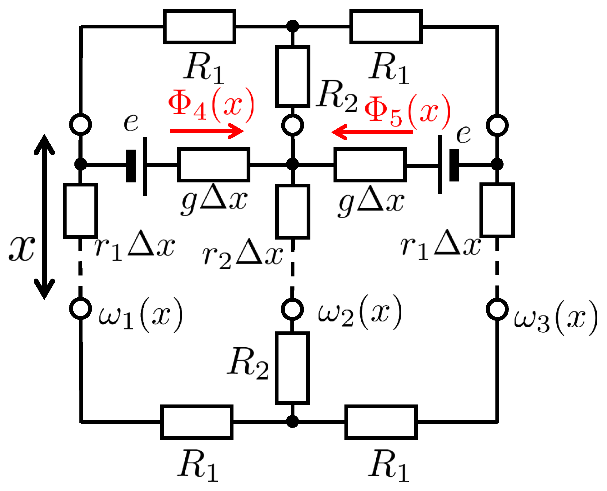
It is thought that the flux of a permanent magnet is stronger at the center than at the edge; Figure 5. As can be seen from this, the interlinkage flux of the armature coil depends upon the position of the coil. It affects high-precision positioning. In this section, the mathematical model is derived using a distributed constant magnetic circuit. The circuit diagram is shown in Figure 8. Where $R_{1,2}$ are the magnetic resistance of each yoke, $r_{1,2}$ are the magnetic resistance per unit length of each yoke, g is the magnetic conductance per unit length of the air gap, e is the magnetomotive force of the permanent magnet, ${\omega }_{1,2,3}$ are the magnetic potential of each point, and ${\mathsf{\Phi }}_{4,5}$ are magnetic flux interlinking the armature coil. When analyzing the distributed constant part of Figure 8 in $\Delta x\to 0$, the second-order differential equation shown at (25) is derived.

$$\begin{array}{cc}\hfill & \frac{d^2}{d{t}^2}\mathit{\omega }\left(x\right)=\mathit{RG}\mathit{\omega }\left(x\right)+\mathit{Rg}e\hfill \\ \hfill & \mathsf{\Phi }\left(x\right)={\mathsf{\Phi }}_4\left(x\right)+{\mathsf{\Phi }}_5\left(x\right)={\mathit{g}}^T\mathit{\omega }\left(x\right)+2ge\hfill \end{array}$$

(25)

where the parameters for (25) are

$$\begin{array}{cc}\hfill & \mathit{\omega }={\left(\begin{array}{ccc}{\omega }_1& {\omega }_2& {\omega }_3\end{array}\right)}^T\hfill \\ \hfill & \mathit{R}=\left(\begin{array}{ccc}{r}_1& 0& 0\\ 0& r_2& 0\\ 0& 0& r_1\end{array}\right)\hfill \\ \hfill & \mathit{G}=\left(\begin{array}{ccc}g& -g& 0\\ -g& 2g& -g\\ 0& -g& g\end{array}\right)\hfill \\ \hfill & \mathit{g}={\left(\begin{array}{ccc}g& -2g& g\end{array}\right)}^T\hfill \end{array}$$

To solve the equation in (25), the hyperbolic function shown in (26) is obtained. Where $\widehat{a}$, $\widehat{b}$, $\widehat{k}$ are the designed parameters of the function, and they are compared with experimental results.

$$\begin{array}{cc}\hfill & \mathsf{\Phi }\left(x\right)=\widehat{a}-\widehat{b}\left(cosh\left(\widehat{k}x\right)-1\right)\hfill \end{array}$$

(26)

To obtain the formula of interlinkage flux as (26), the nonlinear model of VCM is designed. It is shown in (27).

$$\begin{array}{cc}\hfill & \frac{d}{dt}\left(\begin{array}{c}p\\ v\\ i\end{array}\right)\left(t\right)=\left(\begin{array}{ccc}0& 1& 0\\ -{\displaystyle \frac{k}{m}}& -{\displaystyle \frac{c}{m}}& {\displaystyle \frac{\mathsf{\Phi }\left(p\right)}{m}}\\ 0& -{\displaystyle \frac{\mathsf{\Phi }\left(p\right)}{L}}& -{\displaystyle \frac{R}{L}}\end{array}\right)\left(\begin{array}{c}p\\ v\\ i\end{array}\right)\left(t\right)+\left(\begin{array}{c}0\\ 0\\ {\displaystyle \frac{1}{L}}\end{array}\right)u\left(t\right)\hfill \\ \hfill & y\left(t\right)=p\left(t\right)\hfill \\ \hfill & \mathsf{\Phi }\left(p\right)=\widehat{a}-\widehat{b}\left(cosh\left(\widehat{k}p\right)-1\right)\hfill \end{array}$$

(27)

5. Proposed Controller

5.1. Operator Expression of Plant

To design the controller and transform the expression of the plant from state-space to operator, the plant is expressed as the nth-order differential equation without state variables. The plant model is considered as a time-varying of flux. Therefore, it is expressed that adding the element caused the time derivative of flux to the general linear differential equation in (28).

$$\begin{array}{cc}\hfill \stackrel{⃛}{y}\left(t\right)& =-\frac{kR}{mL}y\left(t\right)-\left(\frac{k}{m}+\frac{\mathsf{\Phi }{\left(y\right)}^2}{mL}+\frac{cR}{mL}\right)\dot{y}\left(t\right)-\left(\frac{c}{m}+\frac{R}{L}\right)\ddot{y}\left(t\right)+\frac{\mathsf{\Phi }\left(y\right)}{mL}u\left(t\right)\hfill \\ \hfill & +\frac{\dot{\mathsf{\Phi }}\left(y\right)}{\mathsf{\Phi }\left(y\right)}\left(\ddot{y}\left(t\right)+\frac{c}{m}\dot{y}\left(t\right)+\frac{k}{m}y\left(t\right)\right)\hfill \end{array}$$

(28)

where $\dot{\mathsf{\Phi }}$ is the time derivative of $\mathsf{\Phi }$, and it is expressed in (29)

$$\begin{array}{cc}\hfill \dot{\mathsf{\Phi }}\left(y\right)& =\frac{\partial \mathsf{\Phi }}{\partial y}\dot{y}\left(t\right)\hfill \\ \hfill & =-\widehat{b}\widehat{k}sinh\left(\widehat{k}y\left(t\right)\right)\dot{y}\left(t\right)\hfill \end{array}$$

(29)

Equations (28) and (29) are used as the model for controller design.

5.2. Compensating Robust Stability with Operator-Based Controller

In this section, operator-based feedback control is used to compensate for the robust stability of the plant. First, N and D, which are the right factorizations of P, are derived. Then, two models of the plant are constructed; one for the motion equation and one for the circuit equation. The motion equation is expressed as linear. Therefore, the nonlinear plant model is able to be transformed by a simple linear model design, in which N expresses the motion equation and D expresses the circuit equation, according to (4). N and $D^{-1}$ are designed with the ideas that are expressed in (30).

$$\begin{array}{cc}\hfill N& \left\{\begin{array}{cc}\hfill & {\ddot{x}}_n\left(t\right)=-\frac{c}{m}{\dot{x}}_n\left(t\right)-\frac{k}{m}{x}_n\left(t\right)+\frac{1}{m}w\left(t\right)\hfill \\ \hfill & y\left(t\right)=x_n\left(t\right)\hfill \end{array}\right.\hfill \\ \hfill D^{-1}& \left\{\begin{array}{cc}\hfill & {\ddot{x}}_d\left(t\right)=-\frac{c}{m}{\dot{x}}_d\left(t\right)-\frac{k}{m}{x}_d\left(t\right)+\frac{1}{m}w\left(t\right)\hfill \\ \hfill & \dot{w}\left(t\right)=-\frac{R}{L}w\left(t\right)-\frac{\mathsf{\Phi }{\left(x_d\right)}^2}{L}{\dot{x}}_d\left(t\right)+\frac{\mathsf{\Phi }\left(x_d\right)}{L}u\left(t\right)\hfill \\ \hfill & +\left(k{x}_d\left(t\right)+c{\dot{x}}_d\left(t\right)+m{\ddot{x}}_d\left(t\right)\right)\frac{{\mathsf{\Phi }}^{\prime }\left(x_d\right)}{\mathsf{\Phi }\left(x_d\right)}{\dot{x}}_d\left(t\right)\hfill \\ \hfill & \mathsf{\Phi }\left(x_d\right)=\left\{\begin{array}{c}\widehat{a}-\widehat{b}\left(cosh\left(\widehat{k}{x}_d\right)-1\right)\left(-l\le x_d\le l\right)\hfill \\ \mathsf{\Phi }\left(l\right)\left(\mathrm{other}\right)\hfill \end{array}\right.\hfill \\ \hfill & {\mathsf{\Phi }}^{\prime }\left(x_d\right)=\left\{\begin{array}{c}-\widehat{b}\widehat{k}sinh\left(\widehat{k}{x}_d\right)\left(-l\le x_d\le l\right)\hfill \\ {\mathsf{\Phi }}^{\prime }\left(l\right)\left(\mathrm{other}\right)\hfill \end{array}\right.\hfill \end{array}\right.\hfill \end{array}$$

(30)

In the next step, S and R are designed to satisfy Bézout’s identity (3). Let S be the set identity operator I to simplify the design. Substituting it into (3), R is expressed as (31).

$$\begin{array}{cc}\hfill & N+RD=M\hfill \\ \hfill & R=\left(M-N\right)D^{-1}\hfill \end{array}$$

(31)

In this study, M is designed where $M^{-1}$ is the operator of a first-order low-pass filter (LPF) shown in (32). Where ${\tau }_m$ is the time constant of LPF.

$$\begin{array}{c}\hfill M^{-1}\left\{\begin{array}{cc}\hfill & {\dot{x}}_m\left(t\right)={\tau }_m^{-1}{x}_m\left(t\right)+{\tau }_m^{-1}r\left(t\right)\hfill \\ \hfill & w\left(t\right)=x_m\left(t\right)\hfill \end{array}\right.\end{array}$$

(32)

Substituting N, $D^{-1}$ and M into (31), R is expressed as (33).

$$\begin{array}{cc}\hfill R& \left\{\begin{array}{cc}\hfill & {\ddot{x}}_{r_n}\left(t\right)=-\frac{c}{m}{\dot{x}}_{r_n}\left(t\right)-\frac{k}{m}{x}_{r_n}\left(t\right)+\frac{1}{m}{w}_r\left(t\right)\hfill \\ \hfill & x_{r_m}\left(t\right)={\tau }_m{\dot{w}}_r\left(t\right)+w_r\left(t\right)\hfill \\ \hfill & {\dot{w}}_r\left(t\right)=-\frac{R}{L}{w}_r\left(t\right)-\frac{\mathsf{\Phi }{\left(x_{r_n}\right)}^2}{L}{\dot{x}}_{r_n}\left(t\right)+\frac{\mathsf{\Phi }\left(x_{r_n}\right)}{L}u\left(t\right)\hfill \\ \hfill & +\left(k{x}_{r_n}\left(t\right)+c{\dot{x}}_{r_n}\left(t\right)+m{\ddot{x}}_{r_n}\left(t\right)\right)\frac{{\mathsf{\Phi }}^{\prime }\left(x_{r_n}\right)}{\mathsf{\Phi }\left(x_{r_n}\right)}{\dot{x}}_{r_n}\left(t\right)\hfill \\ \hfill & e\left(t\right)=x_{r_m}\left(t\right)-x_{r_n}\left(t\right)\hfill \\ \hfill & \mathsf{\Phi }\left(x_{r_n}\right)=\left\{\begin{array}{c}\widehat{a}-\widehat{b}\left(cosh\left(\widehat{k}{x}_{r_n}\right)-1\right)\left(-l\le x_{r_n}\le l\right)\hfill \\ \mathsf{\Phi }\left(l\right)\left(\mathrm{other}\right)\hfill \end{array}\right.\hfill \\ \hfill & {\mathsf{\Phi }}^{\prime }\left(x_{r_n}\right)=\left\{\begin{array}{c}-\widehat{b}\widehat{k}sinh\left(\widehat{k}{x}_{r_n}\right)\left(-l\le x_{r_n}\le l\right)\hfill \\ {\mathsf{\Phi }}^{\prime }\left(l\right)\left(\mathrm{other}\right)\hfill \end{array}\right.\hfill \end{array}\right.\hfill \\ \hfill \end{array}$$

(33)

The inverse of R needs to be found since the controller uses $R^{-1}$ according to Figure 9. The operators used in the controller are expressed as (34), deriving the inverse model of R. Where the initial values of all inner-states $x_{rn}$, $x_{rm}$, and $x_m$ and the time derivates of them (e.g., ${\dot{x}}_{rn}$) are 0. They are derived to compute differential equations of themselves.

$$\begin{array}{cc}\hfill R^{-1}& \left\{\begin{array}{cc}\hfill & {\stackrel{⃛}{x}}_{r_n}\left(t\right)=-\left(\frac{c}{m}+{\tau }_m^{-1}\right){\ddot{x}}_{r_n}\left(t\right)-\left(\frac{k}{m}+\frac{c}{m}{\tau }_m^{-1}\right){\dot{x}}_{r_n}\left(t\right)\hfill \\ \hfill & -\frac{k-1}{m}{\tau }_m^{-1}{x}_{r_n}\left(t\right)+\frac{{\tau }_m^{-1}}{m}e\left(t\right)\hfill \\ \hfill & x_{r_m}\left(t\right)=e\left(t\right)+x_{r_n}\left(t\right)\hfill \\ \hfill & {\dot{w}}_r\left(t\right)=-{\tau }_m^{-1}{w}_r\left(t\right)+{\tau }_m^{-1}{x}_{r_m}\left(t\right)\hfill \\ \hfill & u\left(t\right)=\frac{L}{\mathsf{\Phi }\left(x_{r_n}\right)}{\dot{w}}_r\left(t\right)+\frac{L}{\mathsf{\Phi }\left(x_{r_n}\right)}{w}_r\left(t\right)+\mathsf{\Phi }\left(x_{r_n}\right){\dot{x}}_{r_n}\left(t\right)\hfill \\ \hfill & -\left(k{x}_{r_n}\left(t\right)+c{\dot{x}}_{r_n}\left(t\right)+m{\ddot{x}}_{r_n}\left(t\right)\right)\frac{{\mathsf{\Phi }}^{\prime }\left(x_{r_n}\right)}{\mathsf{\Phi }\left(x_{r_n}\right)}{\dot{x}}_{r_n}\left(t\right)\hfill \\ \hfill & \mathsf{\Phi }\left(x_{r_n}\right)=\left\{\begin{array}{c}\widehat{a}-\widehat{b}\left(cosh\left(\widehat{k}{x}_{r_n}\right)-1\right)\left(-l\le x_{r_n}\le l\right)\hfill \\ \mathsf{\Phi }\left(l\right)\left(\mathrm{other}\right)\hfill \end{array}\right.\hfill \\ \hfill & {\mathsf{\Phi }}^{\prime }\left(x_{r_n}\right)=\left\{\begin{array}{c}-\widehat{b}\widehat{k}sinh\left(\widehat{k}{x}_{r_n}\right)\left(-l\le x_{r_n}\le l\right)\hfill \\ {\mathsf{\Phi }}^{\prime }\left(l\right)\left(\mathrm{other}\right)\hfill \end{array}\right.\hfill \end{array}\right.\hfill \\ \hfill S& :b_1\left(t\right)=y\left(t\right)\hfill \\ \hfill M^{-1}& \left\{\begin{array}{cc}\hfill & {\dot{x}}_m\left(t\right)={\tau }_m^{-1}{x}_m\left(t\right)+{\tau }_m^{-1}r\left(t\right)\hfill \\ \hfill & w\left(t\right)=x_m\left(t\right)\hfill \end{array}\right.\hfill \\ \hfill \end{array}$$

(34)

It is indicated that the plant has the right coprime factorization in the section. Therefore, the robust stability of the plant is compensated for by the feedback control indicated in Figure 9 and (34). Furthermore, the operator expressing tracking performance is transformed into a simple linear operator expressed in (4). Therefore, it can use linear control theory to design the tracking controller.

5.3. Proving the Stability of Control System

This system is designed using operator theory. Therefore, if the right factorization of N and D of plant P are coprimes, i.e., Bezout’s identity (3) is satisfied in the proposed system, stability is ensured.

First, $SN$ and $RD$ of this system are derived using (30) and (34). They are derived in the following. Note that the expression for $\mathsf{\Phi }$ is omitted because it is unnecessary for the analysis.

$$\begin{array}{cc}\hfill SN:w\mapsto b_1& \left\{\begin{array}{cc}\hfill & {\ddot{x}}_n\left(t\right)=-\frac{c}{m}{\dot{x}}_n\left(t\right)-\frac{k}{m}{x}_n\left(t\right)+\frac{1}{m}w\left(t\right)\hfill \\ \hfill & b_1\left(t\right)=x_n\left(t\right)\hfill \end{array}\right.\hfill \\ \hfill RD:w\mapsto e& \left\{\begin{array}{cc}\hfill & {\ddot{x}}_d\left(t\right)=-\frac{c}{m}{\dot{x}}_d\left(t\right)-\frac{k}{m}{x}_d\left(t\right)+\frac{1}{m}w\left(t\right)\hfill \\ \hfill & {\ddot{x}}_{r_n}\left(t\right)=-\frac{c}{m}{\dot{x}}_{r_n}\left(t\right)-\frac{k}{m}{x}_{r_n}\left(t\right)+\frac{1}{m}{w}_r\left(t\right)\hfill \\ \hfill & x_{r_m}\left(t\right)={\tau }_m{\dot{w}}_r\left(t\right)+w_r\left(t\right)\hfill \\ \hfill & {\dot{w}}_r\left(t\right)=\frac{\mathsf{\Phi }\left(x_{r_n}\right)}{\mathsf{\Phi }\left(x_d\right)}\dot{w}\left(t\right)-\frac{R}{L}\left(w_r\left(t\right)-\frac{\mathsf{\Phi }\left(x_{r_n}\right)}{\mathsf{\Phi }\left(x_d\right)}w\left(t\right)\right)\hfill \\ \hfill & -\frac{\mathsf{\Phi }\left(x_{r_n}\right)}{L}\left(\mathsf{\Phi }\left(x_{r_n}\right){\dot{x}}_{r_n}\left(t\right)-\mathsf{\Phi }\left(x_d\right){\dot{x}}_d\left(t\right)\right)\hfill \\ \hfill & +k\left(\frac{{\mathsf{\Phi }}^{\prime }\left(x_{r_n}\right)}{\mathsf{\Phi }\left(x_{r_n}\right)}{x}_{r_n}\left(t\right){\dot{x}}_{r_n}\left(t\right)-\frac{{\mathsf{\Phi }}^{\prime }\left(x_d\right)}{\mathsf{\Phi }\left(x_d\right)}\frac{\mathsf{\Phi }\left(x_{r_{r_n}}\right)}{\mathsf{\Phi }\left(x_d\right)}{x}_d\left(t\right){\dot{x}}_d\left(t\right)\right)\hfill \\ \hfill & +c\left(\frac{{\mathsf{\Phi }}^{\prime }\left(x_{r_n}\right)}{\mathsf{\Phi }\left(x_{r_n}\right)}{\dot{x}}_{r_n}^2\left(t\right)-\frac{{\mathsf{\Phi }}^{\prime }\left(x_d\right)}{\mathsf{\Phi }\left(x_d\right)}\frac{\mathsf{\Phi }\left(x_{r_{r_n}}\right)}{\mathsf{\Phi }\left(x_d\right)}{\dot{x}}_d^2\left(t\right)\right)\hfill \\ \hfill & +m\left(\frac{{\mathsf{\Phi }}^{\prime }\left(x_{r_n}\right)}{\mathsf{\Phi }\left(x_{r_n}\right)}{\ddot{x}}_{r_n}\left(t\right){\dot{x}}_{r_n}\left(t\right)-\frac{{\mathsf{\Phi }}^{\prime }\left(x_d\right)}{\mathsf{\Phi }\left(x_d\right)}\frac{\mathsf{\Phi }\left(x_{r_{r_n}}\right)}{\mathsf{\Phi }\left(x_d\right)}{\ddot{x}}_d\left(t\right){\dot{x}}_d\left(t\right)\right)\hfill \\ \hfill & e\left(t\right)=x_{r_m}\left(t\right)-x_n\left(t\right)\hfill \end{array}\right.\hfill \\ \hfill \end{array}$$

(35)

when the initial values of all inner-states (e.g., $x_n$, $x_{r_n}$, …) are 0, it is obtained that $x_d=x_n=x_{r_n}$, ${\dot{x}}_d={\dot{x}}_n={\dot{x}}_{r_n}$, and $w_r=w$. Substituting it into (35), $SN$ and $RD$ are derived as follows.

$$\begin{array}{cc}\hfill SN:w\mapsto b_1& \left\{\begin{array}{cc}\hfill & {\ddot{x}}_n\left(t\right)=-\frac{c}{m}{\dot{x}}_n\left(t\right)-\frac{k}{m}{x}_n\left(t\right)+\frac{1}{m}w\left(t\right)\hfill \\ \hfill & b_1\left(t\right)=x_n\left(t\right)\hfill \end{array}\right.\hfill \\ \hfill RD:w\mapsto e& \left\{\begin{array}{cc}\hfill & {\ddot{x}}_n\left(t\right)=-\frac{c}{m}{\dot{x}}_n\left(t\right)-\frac{k}{m}{x}_n\left(t\right)+\frac{1}{m}w\left(t\right)\hfill \\ \hfill & x_{r_m}\left(t\right)={\tau }_m\dot{w}\left(t\right)+w\left(t\right)\hfill \\ \hfill & e\left(t\right)=x_{r_m}\left(t\right)-x_n\left(t\right)\hfill \end{array}\right.\hfill \\ \hfill \end{array}$$

(36)

Next, $SN+RD$ is derived using (36).

$$\begin{array}{cc}\hfill SN+RD:w\mapsto r^{\prime }& \left\{\begin{array}{cc}\hfill & {\ddot{x}}_n\left(t\right)=-\frac{c}{m}{\dot{x}}_n\left(t\right)-\frac{k}{m}{x}_n\left(t\right)+\frac{1}{m}w\left(t\right)\hfill \\ \hfill & b_1\left(t\right)=x_n\left(t\right)\hfill \\ \hfill & x_{r_m}\left(t\right)={\tau }_m\dot{w}\left(t\right)+w\left(t\right)\hfill \\ \hfill & e\left(t\right)=x_{r_m}\left(t\right)-x_n\left(t\right)\hfill \\ \hfill & r^{\prime }\left(t\right)=e\left(t\right)+b_1\left(t\right)=x_{r_m}\left(t\right)\hfill \end{array}\right.\hfill \\ \hfill \to SN+RD:w\mapsto r^{\prime }& \left\{\begin{array}{cc}\hfill & x_{r_m}\left(t\right)={\tau }_m\dot{w}\left(t\right)+w\left(t\right)\hfill \\ \hfill & r^{\prime }\left(t\right)=x_{r_m}\left(t\right)\hfill \end{array}\right.\hfill \end{array}$$

(37)

This operator is a first-order lead operator. Therefore, it is a unimodular operator, and stability is ensured.

5.4. Tracking Controller

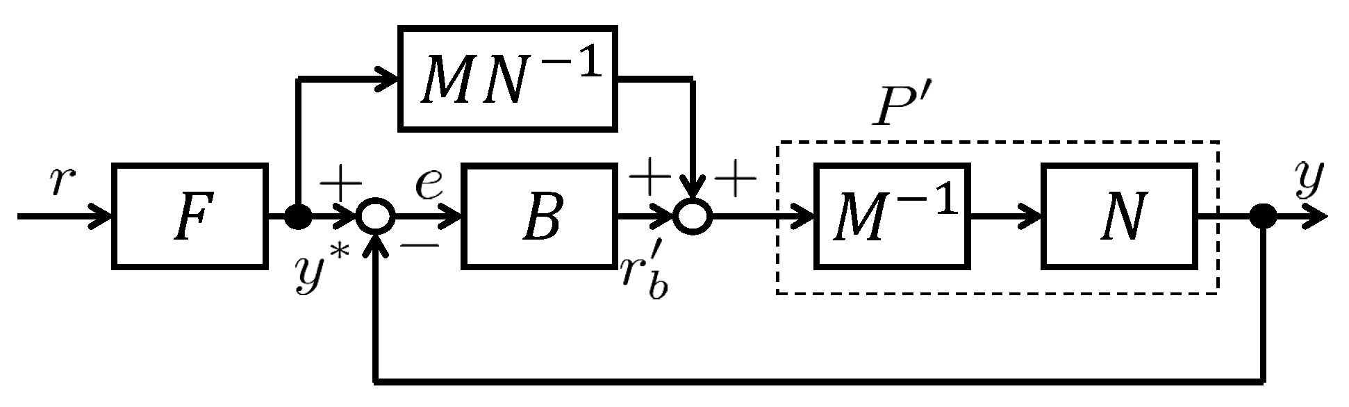
In previous sections, the robust stability is compensated, and the plant model is simplified using an operator-based controller. In this section, the tracking performance of the reference value is compensated for by using a steady-state error compensator. A 2-DOF control is used to compensate for the tracking performance for the reference to achieve a great transient response. A block diagram of this is indicated in Figure 10. From here, the operators F and B are designed to satisfy the stability and tracking performance.

First, F is designed by the desired reference response since it does not depend on feedback operator B. To calculate the reference response using the characteristic, we use (38). According to (38), it depends only on feedforward operator F.

$$\begin{array}{cc}\hfill & y\left(t\right)=N{M}^{-1}M{N}^{-1}F\left(r\right)\left(t\right)\hfill \\ \hfill & y\left(t\right)=F\left(r\right)\left(t\right)\hfill \end{array}$$

(38)

Therefore, F is designed as an ideal operator for reference. It should be noted that F and $M{N}^{-1}F$ must be able to be implemented on a computer. Specifically, they have no differentiator in the operators (called proper in linear theory). The plant of this study is a third-order system since it has the second-order operator N and first-order operator $M^{-1}$. Therefore, F must be designed as a third-order operator. In this study, F is a designed third-order LPF expressed as (39). Where $p^{*}>0$ is the designing parameter determining the tracking time.

$$\begin{array}{c}\hfill F\left\{\begin{array}{c}{\stackrel{⃛}{x}}_f\left(t\right)=-3p^{*}{\ddot{x}}_f\left(t\right)-3p^{*2}{\dot{x}}_f\left(t\right)-p^{*3}{x}_f\left(t\right)+p^{*3}r\left(t\right)\hfill \\ y^{*}\left(t\right)=x_f\left(t\right)\hfill \end{array}\right.\end{array}$$

(39)

The reference response has been designed properly. The next step is to design B to compensate for the tracking performance if the system is affected by uncertain elements and disturbances. To eliminate the effects at steady-state, an integrator is needed at feedback operator B. Therefore, a PID control is used for B because it cannot obtain the desired transient response it is to control only the integrator. It is expressed as (40). Where $K_P$, $K_I$, $K_D$ and $\tau$ are proportional, integral, differential gain and time constant for the differentiator, respectively.

$$\begin{array}{c}\hfill B\left\{\begin{array}{c}{\dot{x}}_i\left(t\right)=e\left(t\right)\hfill \\ {\dot{x}}_d\left(t\right)=-{\tau }^{-1}{x}_d\left(t\right)+{\tau }^{-1}e\left(t\right)\hfill \\ r_b^{\prime }\left(t\right)=K_{P}e\left(t\right)+K_I{x}_i\left(t\right)+K_D{\dot{x}}_d\left(t\right)\hfill \end{array}\right.\end{array}$$

(40)

Calculating Reference-Following Performance

In this section, the characteristic that output y will track to the reference r is indicated to calculate the reference-following performance of the proposed controller.

The nominal plant P (indicated in (27)) is designed sufficiently appropriately, so the effect of uncertainty element $\Delta N$ can be ignored. In this condition, output y is indicated as (4) by an operator-based right coprime factorization. By using a 2-DOF tracking controller, $r^{\prime }$ is expressed as follows.

$$\begin{array}{c}\hfill r^{\prime }\left(t\right)=B\left(F\left(r\right)\left(t\right)-y\left(t\right)\right)+M{N}^{-1}F\left(r\right)\left(t\right)\end{array}$$

Substituting it into (4), the following equation is obtained.

$$\begin{array}{c}\hfill y\left(t\right)=N{M}^{-1}\left(B\left(F\left(r\right)\left(t\right)-y\left(t\right)\right)+M{N}^{-1}F\left(r\right)\left(t\right)\right)\end{array}$$

Tll operators in this equation are linear. Therefore, (41) is expressed via expanding it using the principle of superposition.

$$\begin{array}{cc}\hfill y\left(t\right)=& +N{M}^{-1}BF\left(r\right)\left(t\right)-N{M}^{-1}B\left(y\right)\left(t\right)+F\left(r\right)\left(t\right)\hfill \\ \hfill \left(I+N{M}^{-1}B\right)\left(y\right)\left(t\right)=& \left(I+N{M}^{-1}B\right)F\left(r\right)\left(t\right)\hfill \\ \hfill y\left(t\right)=& F\left(r\right)\left(t\right)\hfill \end{array}$$

(41)

Therefore, output y tracks the reference value r since the operator F is designed with a stationary value of 1.

5.5. Compensating Disturbances Response

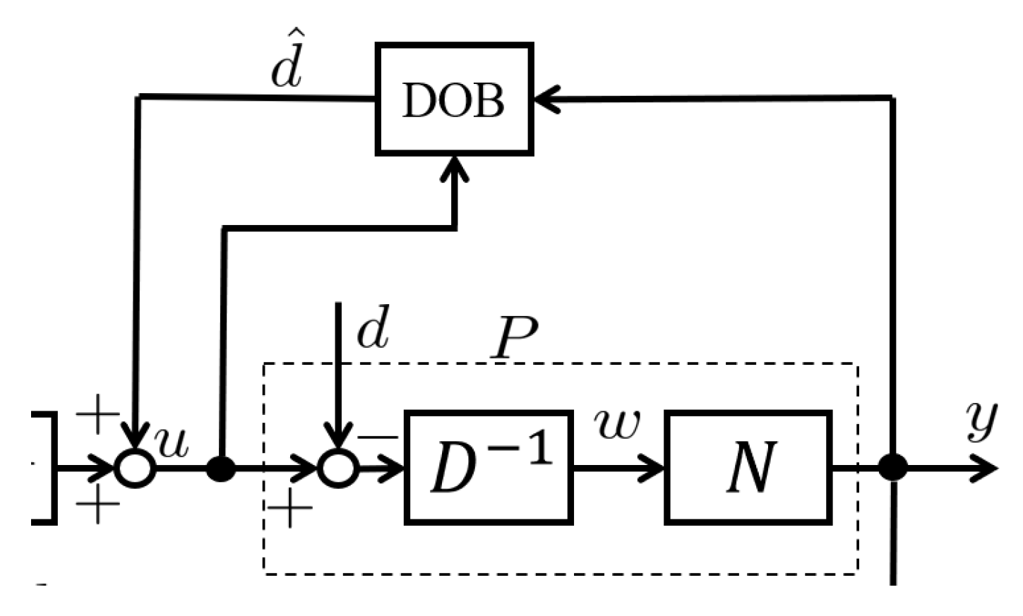
In the previous section, the reference-following performance is compensated. However, the response of the control plant is affected by the disturbance. In this study, the step disturbances, such as friction, are considered. It affects the response, e.g., leading to steady-state error. In this section, the disturbance eliminating controller is proposed using a nonlinear disturbance observer (DOB)-based gradient descent method. The block diagram of the designed observer is expressed in Figure 11. Where d is the input disturbance, and $\widehat{d}$ is the estimated disturbance value by the observer.

The state equation of DOB is as follows.

$$\begin{array}{cc}\hfill & \widehat{\mathit{x}}={\left(\begin{array}{cccc}\widehat{y}& \widehat{v}& \widehat{i}& \widehat{d}\end{array}\right)}^T\hfill \\ \hfill & \frac{d}{dt}\widehat{\mathit{x}}\left(t\right)=\left(\begin{array}{c}\widehat{v}\left(t\right)\\ -\frac{k}{m}\widehat{y}\left(t\right)-\frac{c}{m}\widehat{v}\left(t\right)-\frac{\mathsf{\Phi }\left(\widehat{y}\right)}{m}\widehat{i}\left(t\right)\\ -\frac{\mathsf{\Phi }\left(\widehat{y}\right)}{L}\widehat{v}\left(t\right)-\frac{R}{L}\widehat{i}\left(t\right)-\frac{1}{L}\widehat{d}\left(t\right)+\frac{1}{L}u\left(t\right)\\ 0\end{array}\right)+\mathit{H}\left(t\right)\frac{\partial h\left(\widehat{\mathit{x}}\right)}{\partial \widehat{\mathit{x}}}(y\left(t\right)-h\left(\widehat{\mathit{x}}\right)\left(t\right))\hfill \\ \hfill & h\left(\widehat{\mathit{x}}\right)=\left(\begin{array}{cccc}1& 0& 0& 0\end{array}\right)\widehat{\mathit{x}}\hfill \\ \hfill & \mathsf{\Phi }\left(\widehat{y}\right)=\widehat{a}-\widehat{b}\left(cosh\left(\widehat{k}\widehat{y}\right)-1\right)\hfill \end{array}$$

(42)

Then, $\mathit{H}$ is going to be designed to stabilize the DOB. To stabilize DOB, all eigenvalues $\lambda$ in (43) must be placed on the left side of the complex plane.

$$\begin{array}{cc}\hfill & det\left(\lambda \mathit{I}-{\left.\left(\frac{\partial \mathit{f}(\widehat{\mathit{x}},u)}{\partial \widehat{\mathit{x}}}\left(t\right)-\mathit{H}\left(t\right){\frac{\partial h\left(\widehat{\mathit{x}}\right)}{\partial \widehat{\mathit{x}}}}^2\left(t\right)\right)\right|}_t\right)=0\hfill \\ \hfill & {\forall }_{\lambda },Re\left(\lambda \right)<0\hfill \end{array}$$

(43)

Then, the controller design is completed. The block diagram of the controller is indicated in Figure 12.

6. Simulation and Experiment

6.1. Simulating Response of Reference and Disturbance

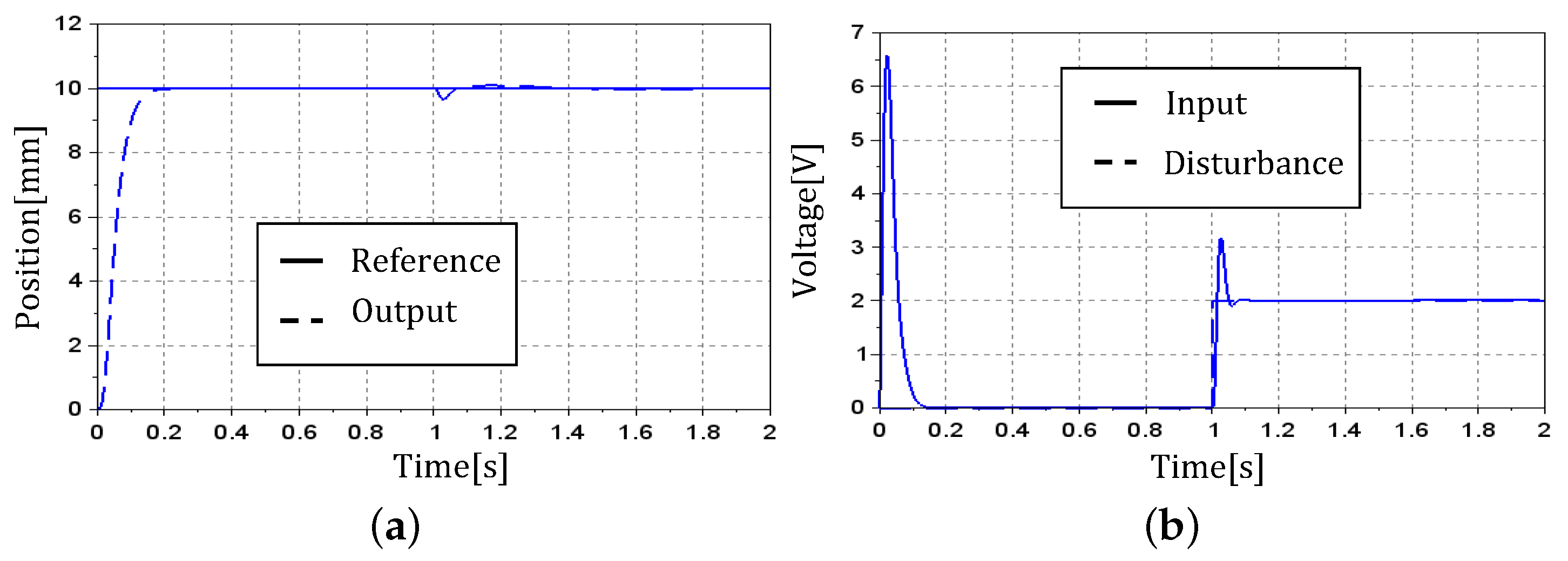
The result of simulating the response to references and disturbances is shown in this section. The inputs of the simulation are set as $r=10\mathrm{mm}$ and $d=2\mathrm{V}(t>2\mathrm{s})$. The sampling time of this simulation is $1\mathrm{ms}$. The parameters of the simulation are indicated in

Table 2. Parameters for the simulation.

Symbol	Value	Unit	Symbol	Value	Unit
m	$1.00$	$\mathrm{kg}$	${\tau }_m$	$0.005$	$\mathrm{s}$
c	$0.10$	$\mathrm{kg}/\mathrm{s}$	$p^{*}$	50	$/\mathrm{s}$
k	$1.10$	$\mathrm{kg}/{\mathrm{s}}^2$	$K_P$	400	$\mathrm{N}/\mathrm{m}$
R	$17.5$	$\mathsf{\Omega }$	$K_I$	5000	$\mathrm{N}/(\mathrm{m}·\mathrm{s})$
L	$27.5$	$\mathrm{mH}$	$K_D$	100	$\mathrm{N}·\mathrm{s}/\mathrm{m}$
$\widehat{a}$	$31.7$	$\mathrm{N}/\mathrm{A}$	$\tau$	$0.002$	$\mathrm{s}$
$\widehat{b}$	$12.0$	$\mathrm{N}/\mathrm{A}$	l	$0.01$	$\mathrm{m}$
$\widehat{k}$	100	$/\mathrm{m}$	$\lambda$	$-200$	$/\mathrm{s}$

. In this condition, the result of the simulation is indicated in Figure 13. The tracking performance for the reference is high-speed, and there are no overshooting and no stationary errors for the feedforward filter F. According to this, the equivalent model $P^{\prime }$ is obtained with high precision by an operator-based controller with a nonlinear model. It can rapidly eliminate the effect of disturbance by feedback operator B and the disturbance observer. It is indicated that a nonlinear DOB can estimate disturbance and stability.

6.2. Comparing with Linear Controller

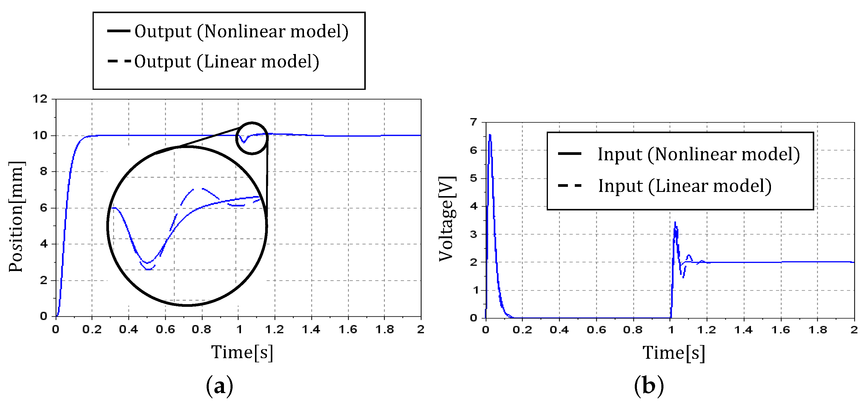
In this section, we compare our design with a design with the same controller for a linear model (24). The linear controller is designed the same as the nonlinear controller. However, its operator $R^{-1}$ is designed as (44), in which the plant model is linear, and DOB is used as a linear observer. The simulation conditions are the same as in the previous section. The results of the simulations are indicated in Figure 14. The results show the performance of the reference cannot find differences. However, in response to the disturbance, a nonlinear model has less oscillation than a linear model, both for input and output. From this, it is confirmed that the proposed model is effective for controlling VCM.

$$\begin{array}{cc}\hfill R^{-1}& \left\{\begin{array}{cc}\hfill & {\stackrel{⃛}{x}}_{r_n}\left(t\right)=-\left(\frac{c}{m}+{\tau }_m^{-1}\right){\ddot{x}}_{r_n}\left(t\right)-\left(\frac{k}{m}+\frac{c}{m}{\tau }_m^{-1}\right){\dot{x}}_{r_n}\left(t\right)\hfill \\ \hfill & -\frac{k-1}{m}{\tau }_m^{-1}{x}_{r_n}\left(t\right)+\frac{{\tau }_m^{-1}}{m}e\left(t\right)\hfill \\ \hfill & x_{r_m}\left(t\right)=e\left(t\right)+x_{r_n}\left(t\right)\hfill \\ \hfill & {\dot{w}}_r\left(t\right)=-{\tau }_m^{-1}{w}_r\left(t\right)+{\tau }_m^{-1}{x}_{r_m}\left(t\right)\hfill \\ \hfill & u\left(t\right)=\frac{L}{\mathsf{\Phi }\left(x_{r_n}\right)}{\dot{w}}_r\left(t\right)+\frac{L}{\mathsf{\Phi }\left(x_{r_n}\right)}{w}_r\left(t\right)+\mathsf{\Phi }\left(x_{r_n}\right){\dot{x}}_{r_n}\left(t\right)\hfill \\ \hfill & \mathsf{\Phi }\left(x_{r_n}\right)=\widehat{a}\hfill \end{array}\right.\hfill \end{array}$$

(44)

6.3. Experimental Results

The results of the experiment in response to the reference and disturbance are shown in this section. In this experiment, it is compared with four conditions. Condition 1: with DOB and operator theory (proposed method); Condition 2: with DOB and without operator theory; Condition 3: without DOB and with operator theory; Condition 4: without DOB and operator theory; In the condition without operator theory, $P^{\prime }$ in Figure 10 is designed as an actual plant P. Therefore, $D{N}^{-1}$ is used as the feedforward controller instead of $M{N}^{-1}$. The reference is $r=3\mathrm{mm}$, and the disturbance is $d=0.2\mathrm{V}$, which are generated by a control program as step signals. The control cycle is $0.1\mathrm{ms}$. The parameters are indicated in

Table 3. Parameters of the experiment.

Symbol	Value	Unit	Symbol	Value	Unit
m	0.0045	kg	${\tau }_m$	0.005	s
c	0.0205	kg/s	p*	100	/s
k	3.08	$\mathrm{kg}/{\mathrm{s}}^2$	$K_P$	10	$\mathrm{N}/\mathrm{m}$
R	$17.5$	$\mathsf{\Omega }$	$K_I$	200	$\mathrm{N}/(\mathrm{m}·\mathrm{s})$
L	$27.5$	$\mathrm{mH}$	$K_D$	$0.65$	$\mathrm{N}·\mathrm{s}/\mathrm{m}$
$\widehat{a}$	$31.7$	$\mathrm{N}/\mathrm{A}$	$\tau$	$0.001$	$\mathrm{s}$
$\widehat{b}$	$12.0$	$\mathrm{N}/\mathrm{A}$	l	$0.005$	$\mathrm{m}$
$\widehat{k}$	100	$/\mathrm{m}$

.

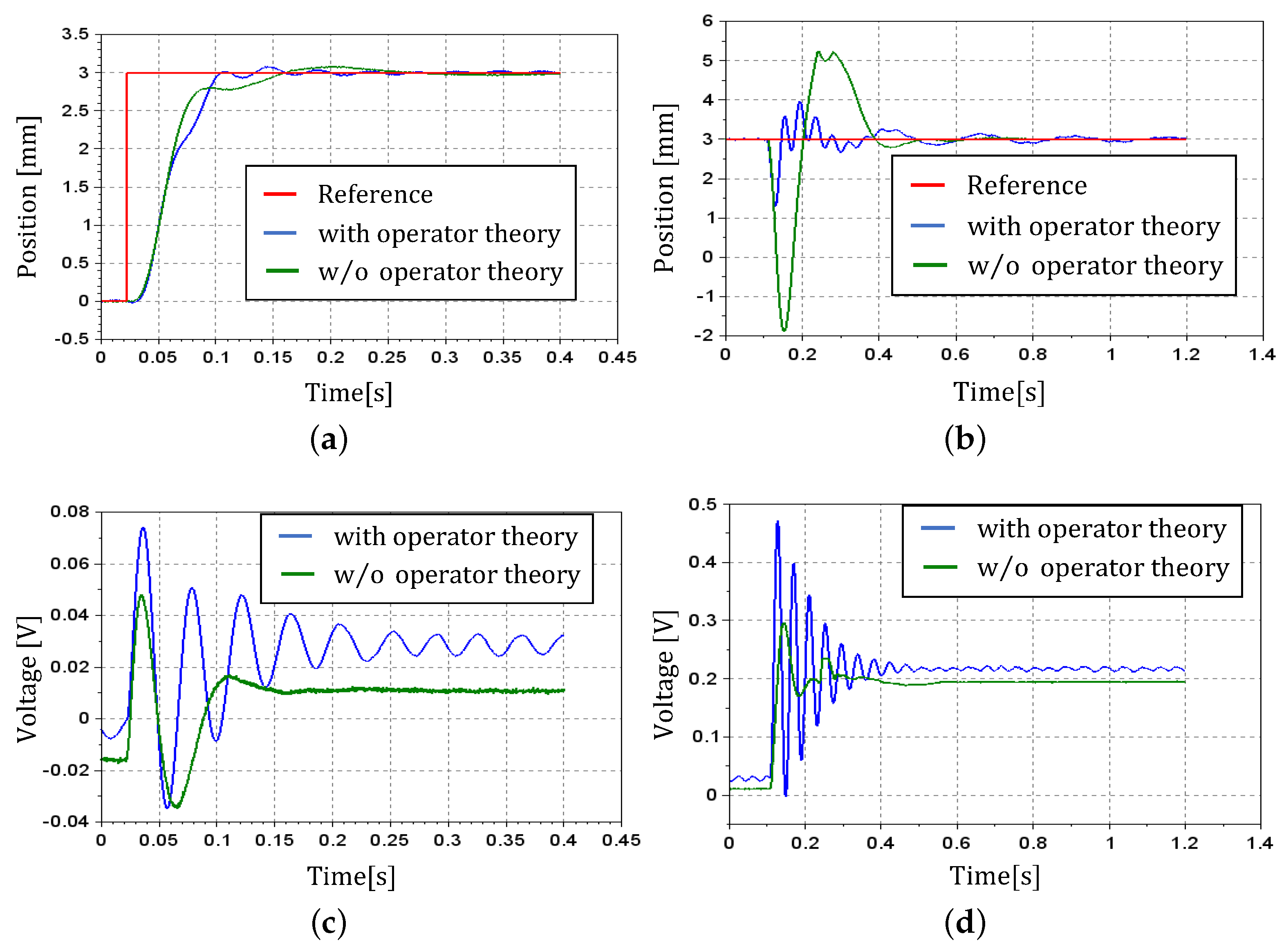
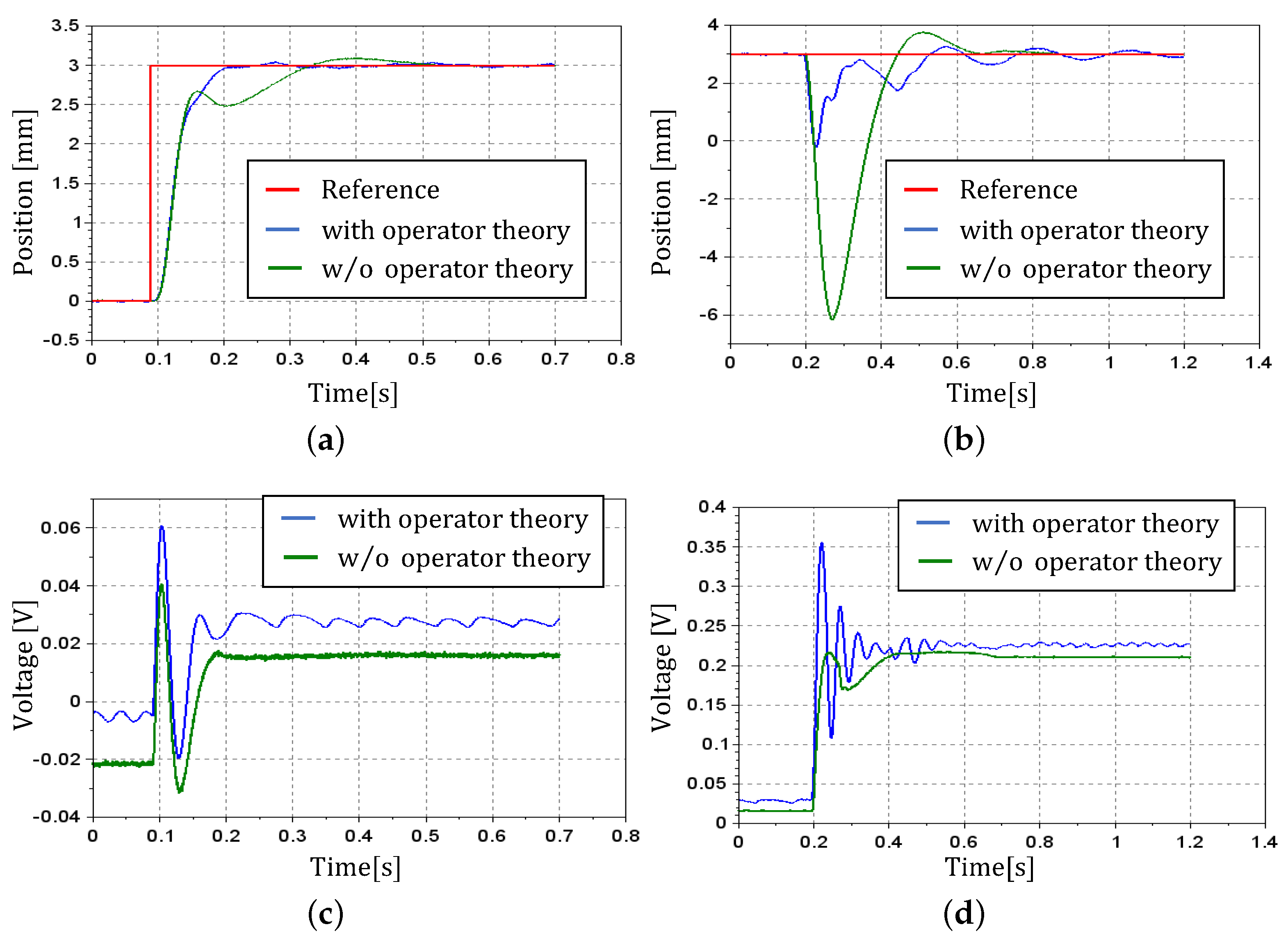
Under these conditions, the results of the experiment with DOB (Conditions 1 and 2) are indicated in Figure 15, and without DOB (Condition 3 and 4) are indicated in Figure 16. In the results, designs with operator theory got faster responses and smaller vibration amplitudes than without operator theory. This is thought to be due to the improved robustness against uncertainties by the operator-based right coprime factorization. In addition, the use of a disturbance observer allows for the faster removal of disturbances. It indicates that the observer is able to estimate the disturbances quickly and accurately.

The maximum overshoot and settling time are measured under each condition for a more detailed analysis. Here, the settling time is defined as the time it takes to get within $2\%$ of the reference value. The data are shown in

Table 4. Overshoot and settling time under each condition for reference.

Conditions:	1	2	3	4
Overshoot ($\mathrm{mm}$)	0.0765	0.0749	0.0386	0.872
Settling time ($\mathrm{s}$)	0.1293	0.1986	0.1057	0.3577

and

Table 5. Overshoot and settling time under each condition for disturbance.

Conditions:	1	2	3	4
Overshoot ($\mathrm{mm}$)	1.70	4.90	3.22	9.16
Settling time ($\mathrm{s}$)	0.9480	0.3857	1.008	0.6114

.

According to the tables, using operator theory achieves a greater settling time for reference than without operator theory. However, when it is combined with DOB, it is less than without operator theory in terms of overshoot. These results may be attributed to the high sensitivity of the operator-based controller to small errors due to the time derivative of $w_r$ in $R^{-1}$. For the same reason, the output fluctuation is reduced for external disturbances, but the settling time is longer due to residual vibration. Comparing the case with and without DOB, both overshoot and settling time are smaller for disturbances when DOB is used. This indicates that DOB is fast and accurate in estimating disturbances, and thus the use of DOB based on the gradient descent method is effective in terms of disturbance elimination. According to these results, the proposed method is effective at improving tracking performance to reference and eliminating the influence of step disturbance.

7. Conclusions

In this study, the nonlinearity of the input-output characteristics of a linear motor is expressed by a proposed model, and the feedback control of the position is performed. Specifically, a more precise model of the linear motor considering the characteristics of the position dependence of the interlinkage flux is expressed using a distributed constant magnetic circuit. In addition, the stability is compensated for and ensured using an operator-based feedback control. According to the experimental results, it is confirmed that the proposed method is effective for linear motor control.

References

- Miyagawa, H.; Yamamoto, A.; Hamamatsu, H.; Goto, S.; Nakamura, M. The mechanical resonance repression control for high–speed positioning of linear motor by using velocity estimated observer of center of gravity. J. Jpn. Soc. Precis. Eng. 2002, 68, 284–290. [Google Scholar] [CrossRef]
- Takahashi, M.; Ogawa, H.; Kato, T. Development of compact maglev nanometer—Scale positioning stage. Precis. Eng. J. Int. Soc. Precis. Eng. Nanotechnol. 2018, 66, 447–448. [Google Scholar]
- Mitsui, Y.; Ahmed, S. Detent force reduction by positional shifting of permanent magnets for a pmlsm without compromising thrust. IEEE Electron. Express 2021, 18, 1–6. [Google Scholar] [CrossRef]
- Manabe, T.; Wakui, S. Production and application of horizontal jerk sensor. In Proceedings of the 2018 International Conference of Advanced Mechatronic Systems, Zhengzhou, China, 30 August–2 September 2018; pp. 305–310. [Google Scholar]
- Nakamura, Y.; Morimoto, K.; Wakui, S. Position control of linear slider via feedback error learning. In Proceedings of the 2011 Third Pacific–Asia Conference on Circuits, Communications and System (PACCS), Piscataway, NJ, USA, 17–18 July 2011; pp. 1–4. [Google Scholar]
- Shao, K.; Zheng, J.; Wang, H.; Xu, F.; Wang, X.; Liang, B. Recursive sliding mode control with adaptive disturbance observer for a linear motor positioner. Mech. Syst. Signal Process. 2021, 146, 107014. [Google Scholar] [CrossRef]
- Zhang, J.; Wang, H.; Cao, Z.; Zheng, J.; Yu, M.; Yazdani, A.; Shahnia, F. Fast nonsingular terminal sliding mode control for permanent-magnet linear motor via elm. Neural Comput. Applic. 2020, 32, 14447–14457. [Google Scholar] [CrossRef]
- Shirani, H.; Wakui, S. Control of an isolated table’s fluctuation caused by supplied air pressure using a voice coil motor. J. Syst. Des. Dyn. 2010, 4, 406–415. [Google Scholar] [CrossRef] [Green Version]
- Liu, T.H.; Lee, Y.C.; Crang, Y.H. Adaptive controller design for a linear motor control system. IEEE Trans. Aerosp. Electron. Syst. 2004, 40, 601–616. [Google Scholar]
- Furukawa, I.; Deng, M. Prescribed performance based nonlinear vibration control of a flexible arm with shape memory alloy actuator. In Proceedings of the 2021 International Conference on Cyber-Physical Social Intelligence, Beijing, China, 18–20 December 2021. [Google Scholar]
- Hoshina, T.; Deng, M. Operator based robust nonlinear position control of linear slider. In Proceedings of the 2021 International Conference on Advanced Mechatronic Systems, Tokyo, Japan, 9–12 December 2021; pp. 1–6. [Google Scholar]
- Jiang, L.; Deng, M.; Inoue, A. Obstacle avoidance and motion control of a two wheeled mobile robot using svr technique. Int. J. Innov. Comput. Inf. Control 2009, 5, 253–262. [Google Scholar]
- Kawamura, S.; Deng, M. Recent developments on modeling for a 3–dof micro–hand based on ai methods. Micromachines 2020, 11, 792. [Google Scholar] [CrossRef] [PubMed]
- Ueno, K.; Kawamura, S.; Deng, M. Operator–based nonlinear control for a miniature flexible actuator using funnel control method. Machines 2021, 9, 26. [Google Scholar] [CrossRef]
- Wen, S.; Deng, M. Operator–based robust nonlinear control and fault detection for a peltier actuated thermal process. Math. Comput. Model. 2013, 57, 16–29. [Google Scholar] [CrossRef]
- Wen, S.; Deng, M.; Inoue, A. Operator–based robust nonlinear control for gantry crane system with soft measurement of swing angle. Int. J. Model. Identif. Control 2012, 16, 86–96. [Google Scholar] [CrossRef]
- Deng, M.; Inoue, A.; Ishikawa, K. Operator–based nonlinear feedback control design using robust right coprime factorization. IEEE Trans. Autom. Control 2006, 51, 645–648. [Google Scholar] [CrossRef] [Green Version]
- Deng, M.; Bu, N. Isomorphism–based robust right coprime factorization of nonlinear unstable plants with perturbations. IET Control Theory Appl. 2006, 4, 2381–2390. [Google Scholar] [CrossRef]
- Wang, A.; Deng, M. Robust nonlinear multivariable tracking control design to a manipulator with unknown uncertainties using operator–based robust right coprime factorization. Trans. Inst. Meas. Control 2013, 35, 788–797. [Google Scholar] [CrossRef]
- Shah, S.; Iwai, Z.; Mizumoto, I.; Deng, M. Simple adaptive control of processes with time–delay. J. Process Control 1997, 7, 439–449. [Google Scholar] [CrossRef]
- Deng, M.; Kawashima, T. Adaptive nonlinear sensorless control for an uncertain miniature pneumatic curling rubber actuator using passivity and robust right coprime factorization. IEEE Trans. Control Syst. Technol. 2016, 24, 318–324. [Google Scholar] [CrossRef]
- Takahashi, K.; Deng, M. Nonlinear sensorless cooling control for a peltier actuated aluminum plate thermal system. In Proceedings of the 2013 International Conference on Advanced Mechatronic Systems, Luoyang, China, 25–27 September 2013; pp. 1–6. [Google Scholar]
- Deng, M.; Wen, S.; Inoue, A. Operator–based robust nonlinear control for a peltier actuated process. Meas. Control J. Inst. Meas. Control 2011, 44, 116–120. [Google Scholar] [CrossRef]
- Sato, H.; Wakui, S. Implementation of disturbance observer without differentiator and suppression of high frequency vibration, international conference on mechanical. In Proceedings of the International Conference on Mechanical, Electrical and Medical Intelligent System 2019, IPS–04–05, Xi’an China, 25–27 October 2019. [Google Scholar]
- Sato, H.; Wakui, S. Adjustment and implementation of a disturbance observer without differentiator. In Proceedings of the 2018 International Conference on Advanced Mechatronic Systems, Zhengzhou, China, 30 August–2 September 2018; pp. 311–315. [Google Scholar]
- Shimizu, K. Nonlinear state observers by gradient descent method. In Proceedings of the 2000 IEEE International Conference on Control Applications, Anchorage, AK, USA, 27 September 2000; pp. 616–622. [Google Scholar]
- Naiborhu, J.; Shimizu, K. Direct gradient descent control for global stabilization of general nonlinear control systems. IEICE Trans. Fundam. Electron. Commun. Comput. Sci. 2000, 83, 516–523. [Google Scholar]
Figure 1.
Operator-based control system.
Figure 2.
Output response using an operator-based control system.
Figure 3.
Nonlinear feedback system including uncertainty.
Figure 4.
Experimental system. (a) Picture, (b) Schematic.
Figure 5.
Structure of VCM.
Figure 6.
Signal flow of VCM.
Figure 7.
Circuit diagram of armature coil-equipped VCM.
Figure 8.
Magnetic circuit model of VCM.
Figure 9.
Operator-based stabilizer.
Figure 10.
Proposed tracking controller.
Figure 11.
Disturbance observer.