
Analytical Study on the Cornering Behavior of an Articulated Tracked Vehicle †


DIMEAS—Department of Mechanical and Aerospace Engineering, Politecnico di Torino, 10129 Turin, Italy
*
Author to whom correspondence should be addressed.
†
This work is an expansion of the paper presented at The 3rd International Conference of IFToMM Italy (IFIT 2020): Tota, A.; Galvagno, E.; Velardocchia, M.; Rota, E.; Novara, A. Articulated Steering Control for an All-Terrain Tracked Vehicle. In Advances in Italian Mechanism Science: Mechanisms and Machine Science 91, Springer, Cham, Switzerland, 2020 (in print).
Machines 2021, 9(2), 38; https://0-doi-org.brum.beds.ac.uk/10.3390/machines9020038
Submission received: 31 December 2020
/
Revised: 4 February 2021
/
Accepted: 5 February 2021
/
Published: 9 February 2021
(This article belongs to the Special Issue Italian Advances on MMS)
Abstract
:Articulated tracked vehicles have been traditionally studied and appreciated for the extreme maneuverability and mobility flexibility in terms of grade and side slope capabilities. The articulation joint represents an attractive and advantageous solution, if compared to the traditional skid steering operation, by avoiding any trust adjustment between the outside and inside tracks. This paper focuses on the analysis and control of an articulated tracked vehicle characterized by two units connected through a mechanical multiaxial joint that is hydraulically actuated to allow the articulated steering operation. A realistic eight degrees of freedom mathematical model is introduced to include the main nonlinearities involved in the articulated steering behavior. A linearized vehicle model is further proposed to analytically characterize the cornering steady-state and transient behaviors for small lateral accelerations. Finally, a hitch angle controller is designed by proposing a torque-based and a speed-based Proportional Integral Derivative (PID) logics. The controller is also verified by simulating maneuvers typically adopted for handling analysis.
1. Introduction
The cornering behavior of tracked vehicles has peculiar characteristics that are different from wheeled vehicles. The steering operation of these vehicles can be accomplished through different mechanisms: skid-steering and steering by articulation. In skid steering, a turning yaw moment is obtained by applying a different longitudinal thrust force between left and right track sides [1,2]. For tracked vehicles with two or more units, the steering operation may be achieved by a relative yaw rotation between units through a specific mechanism on the connecting joint [3,4]. This solution is also preferred to the skid steering since it does not require a thrusts adjustment between the outside and inside tracks so that the resultant forward thrust can be maintained during a turning maneuver, as shown in [5]. Nowadays, articulated tracked vehicles have been widely adopted in several engineering fields, e.g., planetary exploration, military [6], agriculture [7] and construction [8].
The articulated steering is usually accomplished by installing a hydraulic steering system able to provide the power required to overcome vehicle lateral resistances arising during the relative rotation between the two units [8]. The kineto-dynamic behavior of the hydraulic steering mechanism on articulated vehicles was analyzed in [9,10], thus showing a correlation between the hydraulic steering dynamics with the oscillatory articulation response and weaving motion of the vehicle. Moreover, the increasing research focus on autonomous driving has encouraged the development of an automatic steering controller for path tracking or path following applications. Conventional hydraulic steering systems can be replaced or adapted to allow an automatic control: in [11,12,13] a pressure following control is obtained by exploiting the current onboard vehicle hydraulic systems, meanwhile an automatic steering was proposed by [14] through the design of a multifunctional hydraulic steering circuit; an autonomous guidance strategy was also presented in [15] for a load haul dump vehicle where the relationship between vehicle stability and speed is obtained to improve the vehicle dynamic response.
However, these research activities are limited to articulated wheeled vehicles and they cannot be directly extended to articulated tracked vehicles (ATVs) due to the continuous track–terrain contact distribution. Indeed, only few similar studies are available in literature about tracked articulated vehicles. A mathematical model for plane motion to predict the steerability and mobility of an ATV was developed in [5] through numerical simulations. More recently, an improved ATV dynamics model was proposed in [16] by considering the shear stress–shear displacement relation of the soil at the track–terrain interface. The soil deformation on track–soil interaction was also developed in [17], where the side bulldozing effect was also included for improving the model accuracy in simulating the ATV steering operation. A non-linear mathematical model of an ATV was also described by [18,19] where the effect of a hitch angle, i.e., the relative yaw angle between the ATV units, feedback controller was analyzed through steady-state cornering maneuvers. The control of the ATV hitch angle was also adapted for autonomous applications as described in [20], where a path tracking control was designed based on the distance deviation and the heading angle deviation between the ATV and the desired path.
To the best knowledge of the authors, there is a general lack of comprehensive analytical investigation of the ATV transient and steady-state behaviors. Most of the results available in literature are numerically obtained through detailed mathematical models but without any analytical correlation to ATV parameters and operative conditions, e.g., vehicle speed. The activity presented in this paper aims at bridging the gap by providing an analytical approach for analyzing and controlling the ATV cornering response. The paper content represents an extension of the preliminary work introduced in [19] by providing further details related to the non-linear ATV model and by introducing a simplified linearized model, valid for small lateral accelerations. Moreover, the concept of the understeer characteristics, typical of wheeled passenger cars, is also extended to ATV categories. Although the main paper contribution focuses on the methodology for an analytical evaluation of the ATV lateral dynamics behavior, a hitch angle controller is presented to explore the influence of a hydraulic actuation system for the steering operation. The hitch angle controller is designed and calibrated on the non-linear model through an optimization procedure.
The paper structure is organized as follows: a non-linear mathematical model of the ATV is presented in Section 2 by including the effect of rigid bodies planar dynamics, hydraulic steering dynamics, and angular tracks dynamics. The ATV model is then linearized and an analytical solution for the transient and steady-state responses is provided for small lateral accelerations in Section 3. A hitch angle controller is then designed in Section 4 to achieve the desired performance. The controller is then validated through simulations with the non-linear model. Finally, some conclusions are drawn in Section 5.
2. ATV Non-Linear Mathematical Model
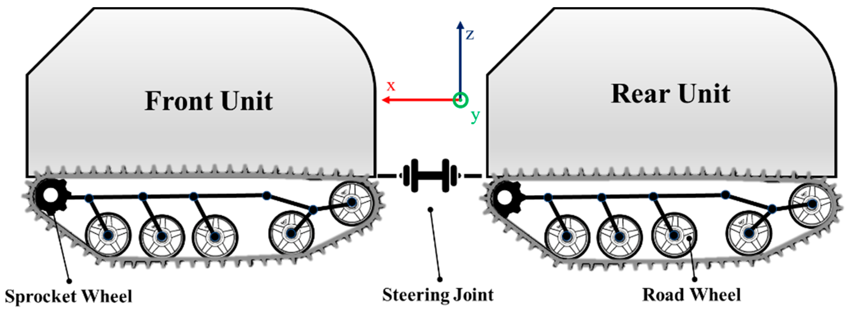
A simplified schematic of the ATV considered within the rest of the paper is reported in Figure 1.
The vehicle architecture is characterized by two units connected through a multi degrees of freedom steering joint. The front unit hosts the driveline components so that the second unit may fulfill the payload functionalities of goods and personnel transportation. The weight of each ATV unit is supported by four or five couples of road wheels. Each road wheel is connected to the hull through a torsion bar suspension system that, together with the set of bushing, represents the elastic-damping components of the ATV. The road wheels are driven by the two sprocket wheels of each unit through a track mechanism. The engine torque is assumed to be equally distributed between the two units and further split in equal parts between the two sprocket wheels of each unit. The ATV steering operation is entrusted to a hydraulic system mounted on the steering joint that provides a steering torque to each unit through the regulation of a flow rate proportional valve.
The ATV dynamics was analyzed through a non-linear mathematical model with eight degrees of freedom (8-DOF) by including the longitudinal, lateral and yaw motion of the front unit, the yaw motion of the rear unit and the angular motion of the four sprocket wheels. The main assumptions for the ATV non-linear model are:
- the two units are considered as rigid bodies with mass and and moment of inertia around the vertical axis through the center of gravity (CoG) and ;
- the road is considered rigid and flat (the effect of terrain slopes or sinkage is neglected);
- the continuous track–terrain contact force distribution is discretized with four contact points for each track;
- the steering joint is considered as an ideal yaw rotational hinge placed at a distance of from the front CoG and from the rear CoG;
- the front and rear tracks width is equal to ;
- the number of road wheels is for each track;
- flexible deformation of the tracks is not considered.
2.1. Rigid Bodies Dynamics
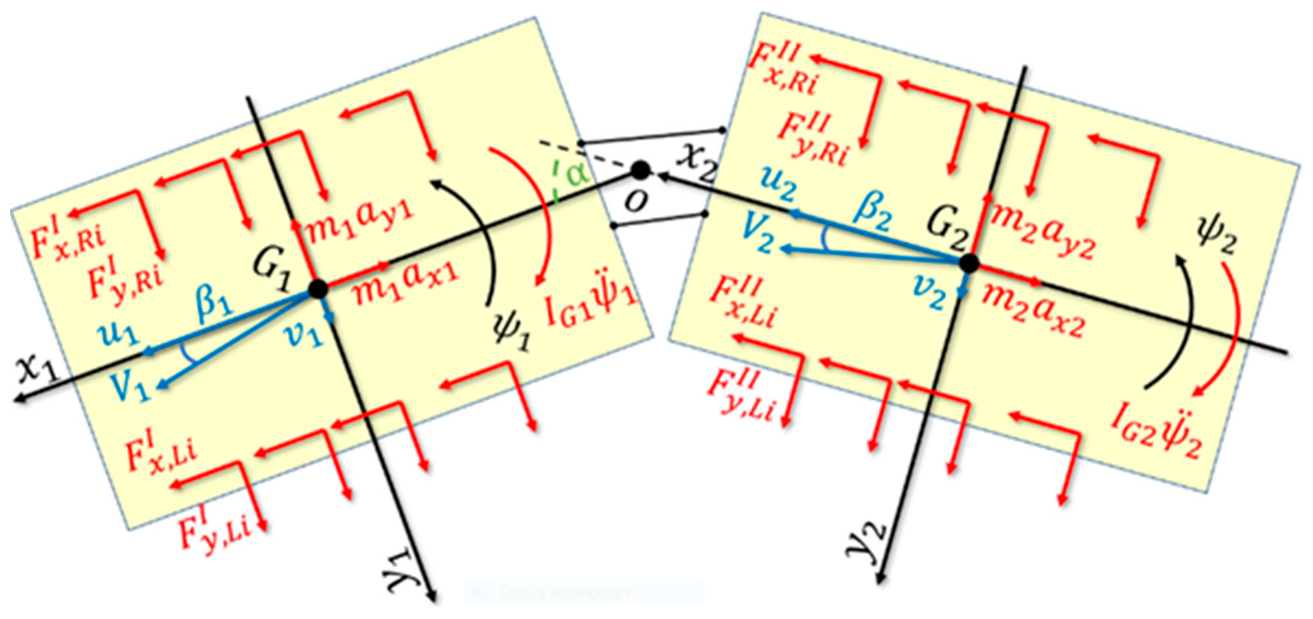
The free body diagram for the ATV planar motion modelling is shown in Figure 2 where a moving reference coordinate system is centered in the front unit CoG and a second moving reference coordinate system is placed in the rear unit CoG.
The ATV longitudinal and lateral equilibrium equations are described by (see also [18]):
where and are the front unit longitudinal and lateral acceleration components; and are the rear unit longitudinal and lateral acceleration components; and are the front unit longitudinal and lateral velocity components; and are the rear unit longitudinal and lateral velocity components. Front and rear velocity vectors, and , are inclined by an angle of and with respect to the corresponding longitudinal direction. and are the yaw angles of the front and rear units, respectively. represents the hitch angle between the two ATV units. and represent the longitudinal force components between the track and the terrain in the road wheel contact point for the front and rear units, respectively. and represent the lateral force components between the track and the terrain in the road wheel contact point for the front and rear units, respectively; is the longitudinal component of the aerodynamics force.
The front and rear yaw moment balance equations are described by:
where and are the front and rear yaw moments generated by the track–terrain forces for the front and rear units, respectively. and are the distances between the axle to the front and rear CoG, respectively, and they are assumed positive if placed in front of their respective CoG; is the steering torque applied by the hydraulic system.
2.2. Track Angular Dynamics
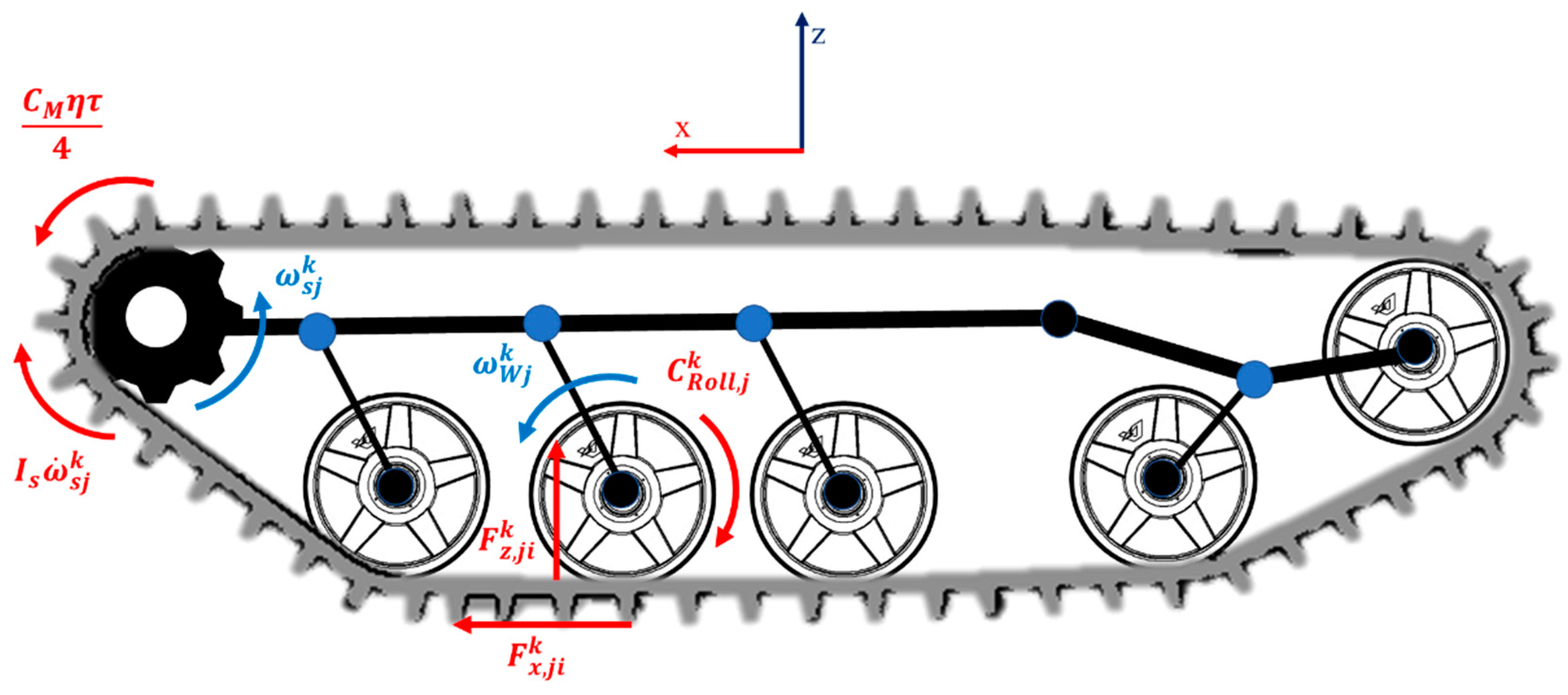
Each track rotational dynamics is described by the free body diagram in Figure 3.
The rotational equilibrium is expressed by:
where is the angular speed of the sprocket wheel and is the road wheel angular speed on the left/right ( side of the unit. and are the sprocket wheels and road wheels radius, respectively. is the engine torque, is the overall transmission efficiency, is the transmission ratio between engine shaft and each sprocket wheel. is the dynamic vertical force on each road wheel. is the equivalent moment of inertia around each sprocket wheel axis and includes all main inertial contributions of the whole powertrain system. Each track rolling resistance is described with a hyperbolic tangent function by introducing the constant coefficient and the track speed () dependent coefficient . Finally, is a pre-defined threshold for the hyperbolic tangent shape factor.
2.3. Track–Terrain Contact Model
The track–terrain contact distribution is modeled by an equivalent finite number of contact patches equal to the number of road wheels [21]. Both contact patch force components and are modeled as hyperbolic tangent functions, depending on their longitudinal slip ratios and slip angles :
where the coefficients , and , are introduced to consider the saturation of the available adhesion to the vertical load. The peak longitudinal and lateral forces occur at and at , respectively. and coefficients enable the longitudinal/lateral combined slips influence.
Each road wheel slip ratio and slip angle is defined as:
where and are, respectively, the longitudinal and lateral components of the road wheel in the side of the unit.
2.4. Dynamic Vertical Forces
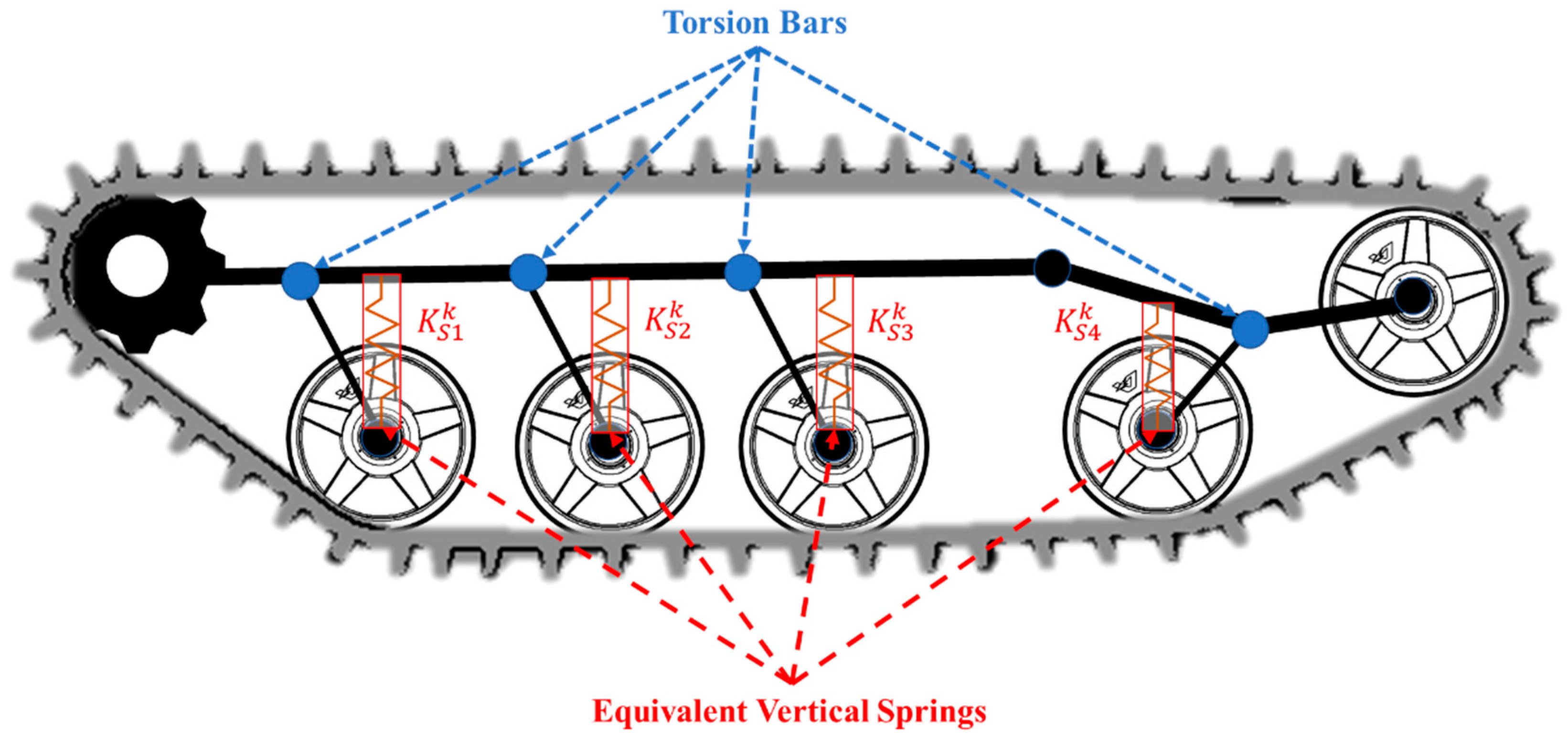
The vertical forces on each road wheel are calculated as the sum of the static and the dynamic load contributions. The static load contribution is evaluated by considering the mass distribution among the four axles of each unit. Due to the statically indeterminate nature of the problem, i.e., cantilever beam supported by a redundant number of constraints, the mass distribution is correlated to the suspension system between the sprung (ATV hull) and the unsprung (track mechanisms) masses. Indeed, each road wheel is connected to the ATV hull by a torsion bar, as shown in Figure 4.
Each torsion bar reacts to the relative motion between the road wheel and the ATV hull, thus behaving as an equivalent vertical spring. The following assumptions are considered for the ATV suspension system:
- Each suspension torsion bar is modeled with a linear characteristic of the equivalent spring deflection.
- Each equivalent spring has no static preload.
- The static deflection is equal for each spring of the same unit (no static pitch and/or roll).
- The corresponding right and left springs of each unit’s axle share the same stiffness value.
Under these assumptions, the static load contribution is then calculated as:
where and are the equivalent vertical spring stiffness for the front and rear units, respectively; and represent the mass distribution on the axle for the front and rear units, respectively. It is remarkable to note that the assumptions made for the ATV suspension system imply that the static mass distribution corresponds to the spring stiffness distribution among each unit’s axle.
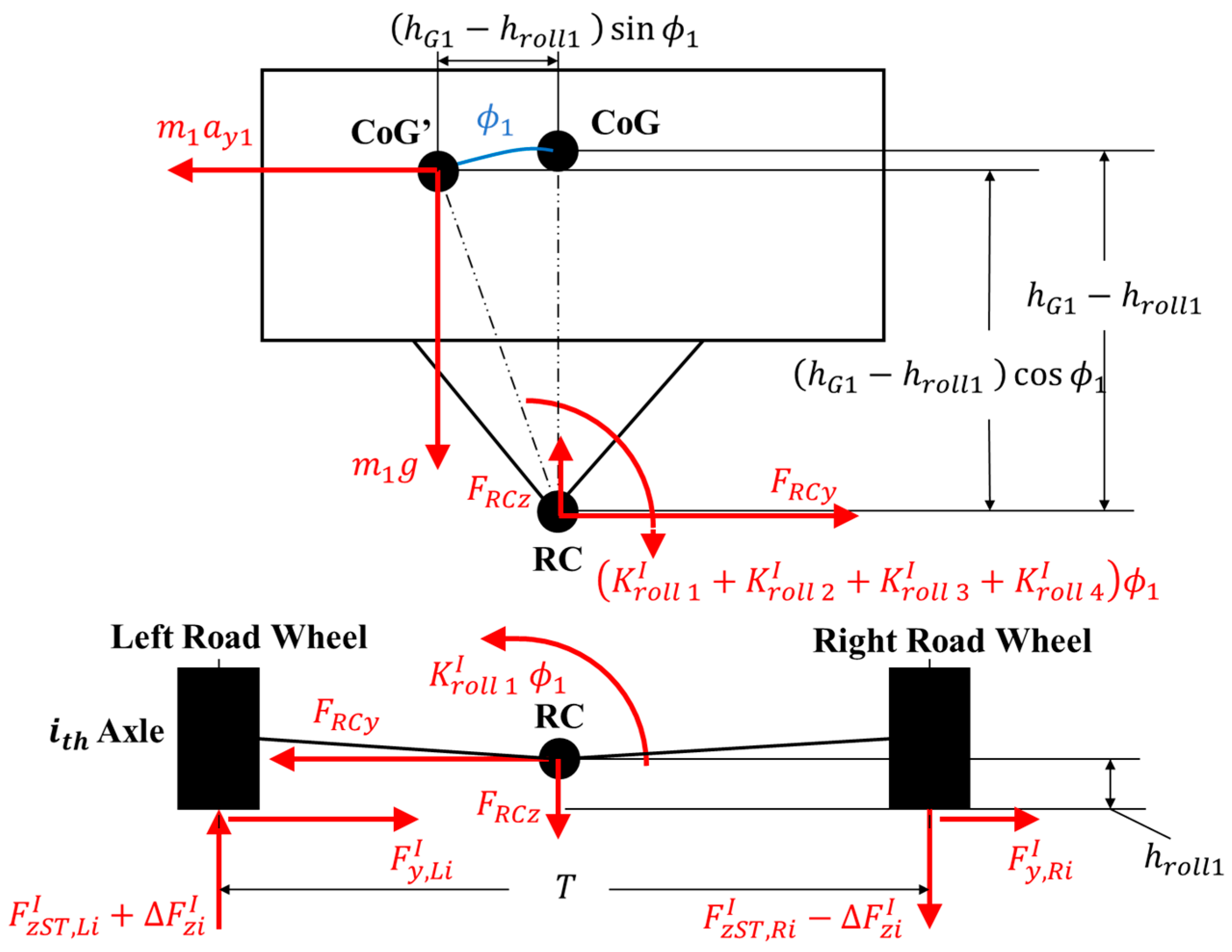
During cornering maneuvers, the lateral acceleration implies a load transfer between the inside and outside tracks for the front unit, , and for the rear unit, . Even if the roll dynamics is not included in the model, the steady-state roll angle represents an internal variable required to evaluate the spring deflection on each unit’s track. The steady-state roll angle is calculated through the moment balance equation of each unit sprung mass around the correspondent roll axis, assumed in a fixed position from the ground.
By assuming small roll angles, i.e., neglecting the distance between CoG and CoG’ in Figure 5, the moment balance equation of each unit sprung mass around its respective roll axis is expressed by:
where and are the roll angles for the front and rear units, respectively; and are the roll axis height for the front and rear units, respectively; and represent the equivalent roll stiffness produced by the two side springs of each axle for the front and rear units, respectively.
The moment balance equation of each unsprung mass around the roll axis provides the lateral load transfer on each axle for the front () and rear () units, as shown in the free body diagram of Figure 5:
By assuming and the load transfer on each axle for the front and rear units is finally defined as:
Equation (11) states the load transfer due to lateral acceleration is distributed as the mass distribution among each unit’s axles. Finally, the total vertical force on each track road wheel for the front and rear units is expressed by:
where the sign of the lateral load transfers and is referred to the left ( or to the right ( side of the front and rear units, respectively, as shown in Figure 5.
2.5. Hydraulic Steering System
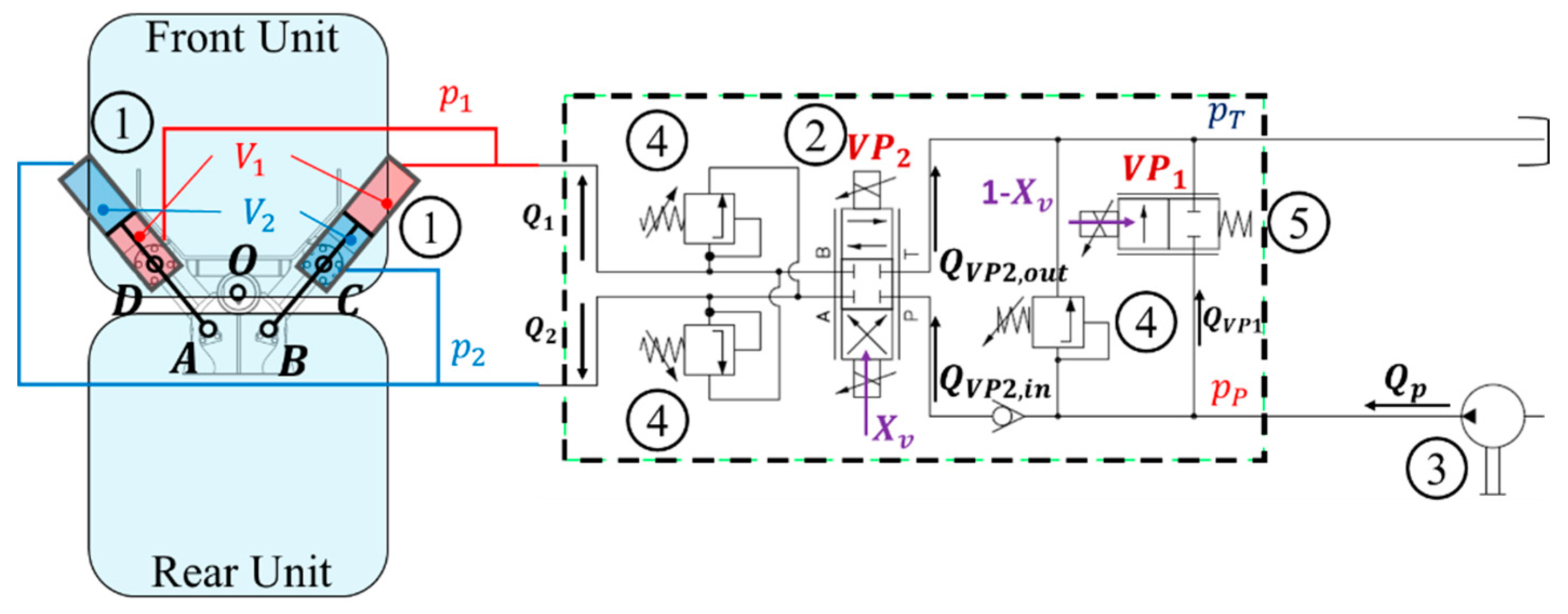
An example of the hydraulic steering circuit is represented in Figure 6.
Two hydraulic cylinders are linked to the front unit through and hinges and their piston rods are linked to the rear unit through and hinges. The fluid pressure and between the cylinder chambers depends on flow rates and controlled by a flow rate proportional valve through the regulation of the command. A constant displacement pump provides the flow rate to cope with the valve request, . The excessive flow rate, , is absorbed by a second flow rate proportional valve that receives the complimentary command . This solution also prevents the pump delivery pressure from growing excessively. For safety reasons, all pressures are saturated by pressure relief valves.
The steering torque is generated by the two hydraulic piston forces as results of pressure and by:
where and are, respectively, the minimum distance of the right and the left piston rods from the hinge (see Appendix A for their analytical expression). and represent the right and left forces, respectively, applied by the corresponding piston rod to ATV bodies:
where is the cylinder bore area and is the piston rod area. is the damping coefficient due to the hydraulic fluid. and are the right and left piston rod extension/compression speeds, respectively (see Appendix A for their analytical expression).
Pressure , and dynamics are defined by the following expressions:
where is the fluid bulk modulus. and are the equivalent cylinder chambers corresponding to , , respectively. Their variation is kinematically imposed on the ATV bodies’ dynamics (see Appendix A for their analytical expression). is the equivalent pipes volume used for the pump pressure, , dynamics. and are the flow rates delivered to chambers and . and when otherwise and . and are the flow rates through the valve pump-connected and tank-connected ports, respectively. is the flow rate delivered through the valve. , and are calculated by:
where is the coefficient of discharge; is and maximum opening valve area. pressure drops are and when otherwise and . pressure drop is .
2.6. Stable Equilibrium Points
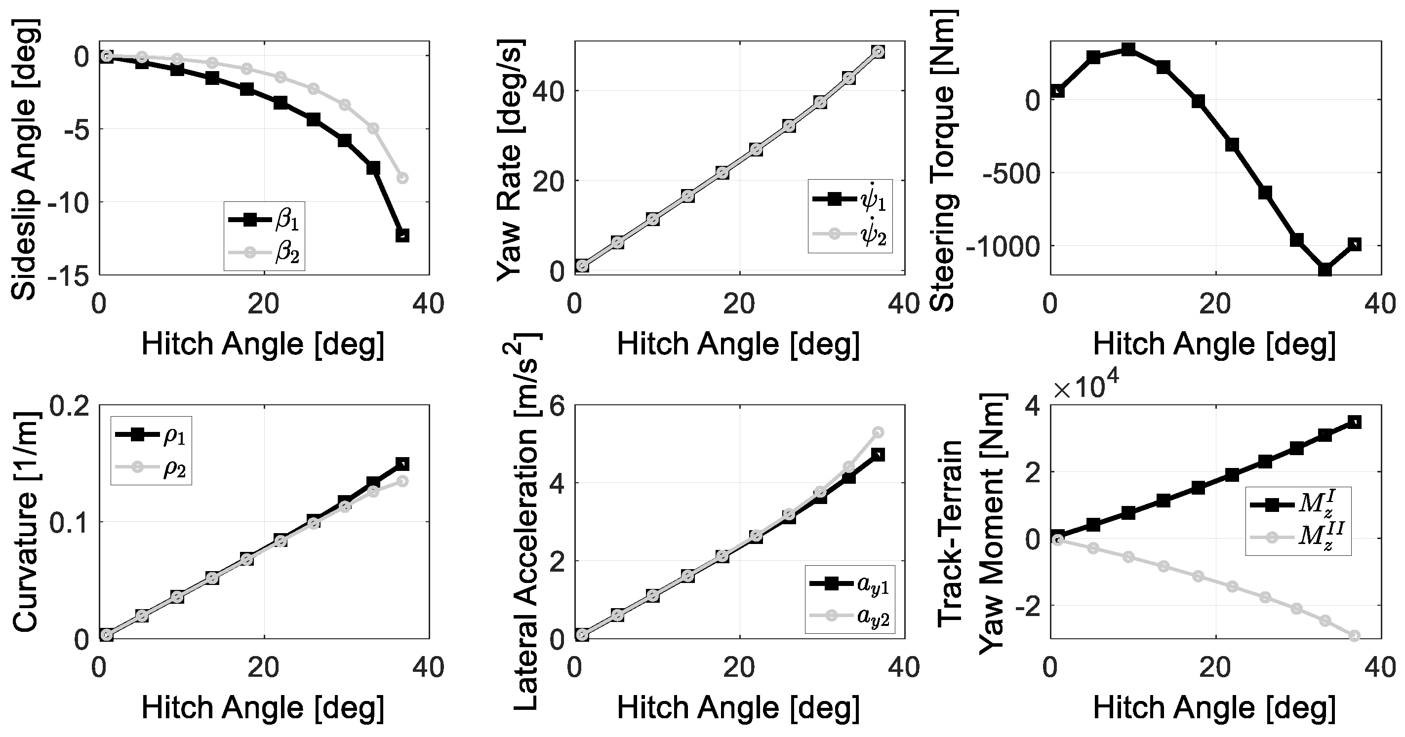
The ATV non-linear model was implemented in MATLAB® and Simulink® environments. The ATV equilibrium conditions were then obtained and represented as characteristic plots between the desired quantities versus the hitch angle, as shown in Figure 7.
Each subplot marker in Figure 7 (square markers refer to the front unit quantities and circle markers to the rear unit) represents an ATV equilibrium condition. Sideslip angles, yaw rates, curvatures, lateral accelerations, and yaw moments characteristics show a linear dependence at least for a limited range of the hitch angle. On the other hand, the relation between the steering torque and the hitch angle is strongly non-linear. The presence of a peak, occurring at 10 deg for km/h, represents a critical point for the relation between the hitch angle and the steering torque: before the peak, the steering torque monotonically increases with the hitch angle, meanwhile, after that peak, an increment of the hitch angle will cause a reduction of the steering torque. This trend leads to an inversion of the steering torque sign that can cause an ATV jackknifing effect for higher hitch angles (see also [18]). Based on these simulation results, a linearized model of the ATV in different equilibrium points may simplify the analysis of the vehicle lateral dynamics.
3. Linearized ATV Lateral Dynamics Model
This section aims to present a linearized version of the ATV non-linear model for lateral dynamics analysis. Since the paper focus is on lateral dynamics, the following hypothesis are considered within the rest of the paper:
- 1.
- Decoupled lateral and longitudinal dynamics: only Equations (2)–(4) are considered for the linearized ATV model and
- 2.
- Neglected longitudinal acceleration and rear unit longitudinal force ;
- 3.
- The longitudinal speed of the front unit is considered a time-independent quantity: is kept constant during each simulation/maneuver.
The effect of the hydraulic steering dynamics, introduced for the non-linear model in Equation (15), was not included in the linearized ATV model: an ideal actuator is assumed for the steering operation so that the actuator applies a desired steering torque with an infinite torque bandwidth that is not influenced by the internal feedback between the actuator and system dynamics. This represents a strong hypothesis since the actuation system may influence the overall vehicle dynamics, but the main purpose of the ATV linearized model is to analyze only the ATV rigid bodies dynamics. The effect of the hydraulic steering dynamics is partially assessed through numerical simulations with the non-linear model in Section 4, where the hydraulic pressure dynamics influences the design of the hitch angle controller.
Equations (2)–(4) show that it is convenient to introduce the axle forces instead of single road wheel contact forces. Given the ATV geometrical symmetry, the left and right road wheels of each axle have almost the same slip angle value () so that the axle lateral force for each unit is calculated as follows:
where is the equivalent slip angle of the axle for the unit:
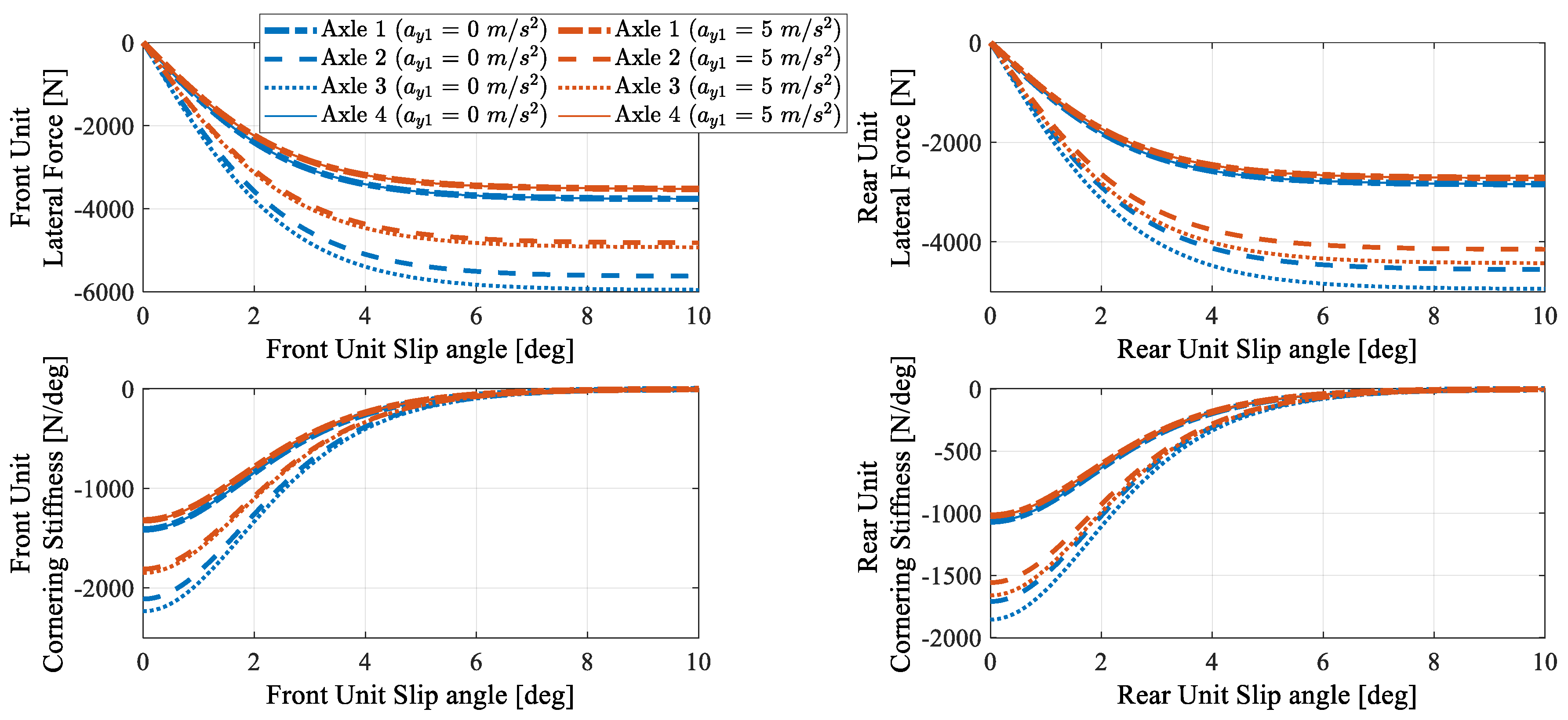
Each axle characteristics , together with their cornering stiffness, are reported in Figure 8 for the front unit (left subplot) and the rear unit (right subplot).
The axle force characteristics shows a linear behavior for small slip angles, which tends to saturate for higher values. Based on that, each axle lateral force in Equation (17) is linearized around the linearization point identified by :
where , and represent the value of the axle lateral force, slip angle and cornering stiffness, respectively, calculated at the linearization point. The cornering stiffness is expressed as:
where and represent the left and right vertical loads, respectively, on each road wheel calculated at the linearization point. By introducing the track–terrain lateral forces linearization and by considering that , the ATV lateral and yaw dynamics is given by:
where the vector collects all the terms related to the linearization point in Equation (20). The rear unit vehicle speed components, and , are kinematically related to the front unit vehicle speed by the following relations:
By substituting Equation (25) into Equations (21)–(23), the following non-linear system of four equations is obtained:
where is the states vector and is the input from the hydraulic steering system.
The ATV dynamics with linear track–terrain lateral forces described in Equation (26) is still non-linear due to the presence of trigonometric functions and states/input products. These non-linearities are then simplified by introducing the first order Taylor expansion around the point :
The matrices , and represent the state, the input and the linearization matrices and contain vehicle geometrical and inertial parameters, axles cornering stiffness and the front unit longitudinal speed .
The first step for analyzing the system dynamics is the identification of the steady-state equilibrium condition so that . A stable ATV steady-state cornering behavior is characterized by a constant hitch angle, i.e., , meaning that the ATV is behaving as a single solid unit with a steering joint locked at a constant hitch angle . The ATV steady-state equilibrium is then obtained from Equation (27) by:
where , and represent the steady-state front unit lateral speed, vehicle yaw rate and hitch angle, respectively.
Analytical Solution for Small Lateral Accelaratons
The analysis of the linearized system described by Equation (27), and its steady-state solution in Equation (28), is carried out by considering a null linearization point , i.e., and . This hypothesis is well representative for small ATV front unit lateral accelerations (). The general expression of Equation (27) can be linked to the characteristic matrices of the dynamic system under investigation:
where matrices , and are defined by:
Equation (28) provides the steady-state relation from the input steering torque to the front lateral speed (or, equivalently, the front sideslip angle ), the ATV yaw rate () and the hitch angle . Nevertheless, the steady-state characteristics vs. and vs. represent a more attractive solution from the steering controller point of view. The explicit dependence of is removed by subtracting the third equation to the second one in Equation (29), thus obtaining the relation among the three states , and :
where , , , and are the speed-dependent coefficients defined by:
The steady-state response is then computed by solving the algebraic system of equations in Equation (33):
where and represent the steady-state sideslip angle and yaw rate gains, respectively.
The steady-state gains of rear sideslip angle , front lateral acceleration , front curvature , front axle slip angles and rear axle slip angles are calculated from and :
The ATV linearized model for small lateral accelerations, through Equations (29), (35) and (36), is then analyzed by providing a realistic parametrization in Table 1.
It is worth noting that each axle cornering stiffness is evaluated for a constant vertical force equal to the static contribution, which represents a realistic assumption if small lateral accelerations are considered.
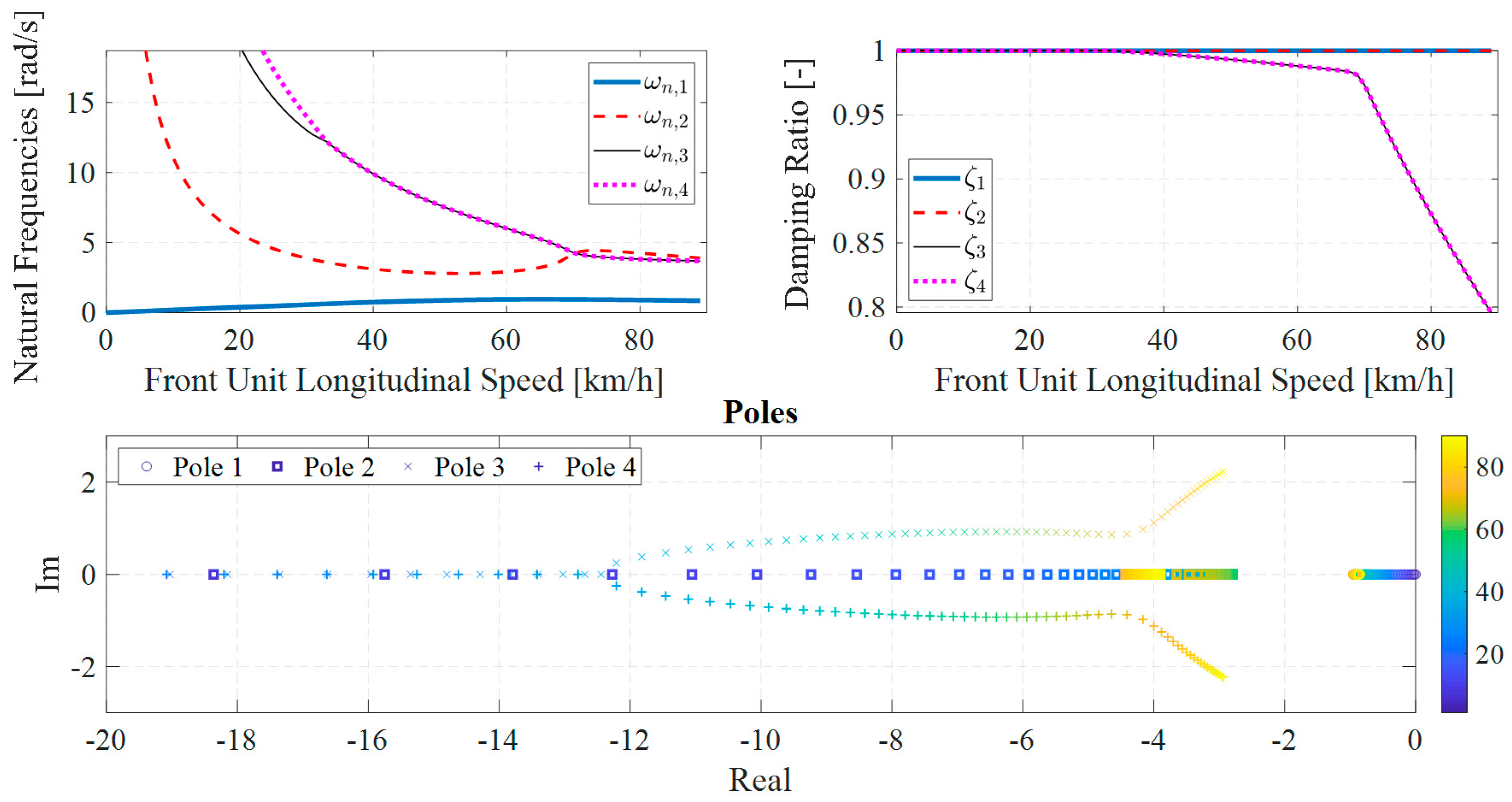
Matrices and in Equation (29) are still influenced by the ATV front longitudinal speed . Despite the assumption of constant speed for the linearized mode, plays an important role for ATV lateral stability and dynamics. The linear model dynamics was then investigated by using the modal analysis, as shown in Figure 9, where the poles, the natural frequencies and the damping ratios are reported as functions of vehicle speed.
All damping ratios are positive, hence the ATV linear model is stable in the whole speed range. The lower natural frequency increases with ATV longitudinal speed up to 65 km/h, where a peak value of 1 rad/s is reached, after which it tends to slightly reduce for higher speed values. The first two poles are real and negative in the whole operative speed range; meanwhile, the third and the fourth eigenvalues are real and distinct for low vehicle speed, while they form a couple of complex conjugate eigenvalues for speeds greater than 33 km/h.
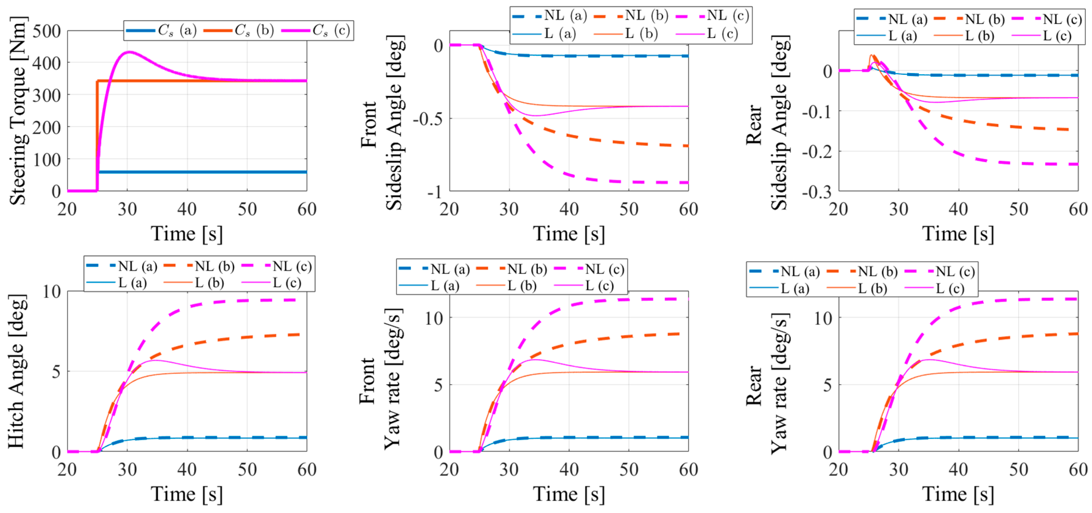
To evaluate the validation range of the linearized ATV model, a step steering torque was applied to both linear and non-linear models to compare their transient and steady-state responses. Simulation results are shown in Figure 10 for three different steering torque histories.
The steering input torques were selected to reach three stable operative points from the steady-state characteristics between steering torque and hitch angle in Figure 7: a step steering torque of 59 Nm (a), a step steering torque of 343 Nm (b), and a smoothed step steering torque of 343 Nm where an overshoot of 432 Nm is imposed during the initial phase. The perfect match between the non-linear and linear responses to the steering torque (a) shows that the assumptions behind the linearization procedure are verified for an ATV operative range characterized by low speed and hitch angle values. When a higher steering torque is applied, e.g., input (b), the starting phase of transient response is still well described by the linear model, but its steady-state response is not aligned with the non-linear model. This result is justified by the selection of the linearization point in the origin of the state space: the more the state deviation from the state space origin, the lower the accuracy level of the linear model in approximating the ATV non-linearities. The non-linear characteristics between the steering torque and the hitch angle is well emphasized by the different response between the linear and the non-linear models to the steering input (c). Indeed, the steering input (c) is designed to reach the same final value of the steering step (b) but with a different time history that aims at moving from the left to the right side of the maximum peak in the characteristics shown in Figure 7. Even if the final value of the steering torque (c) is the same as (b), the steady-state hitch angle from the non-linear model is higher; meanwhile, the linear model approaches the same hitch angle.
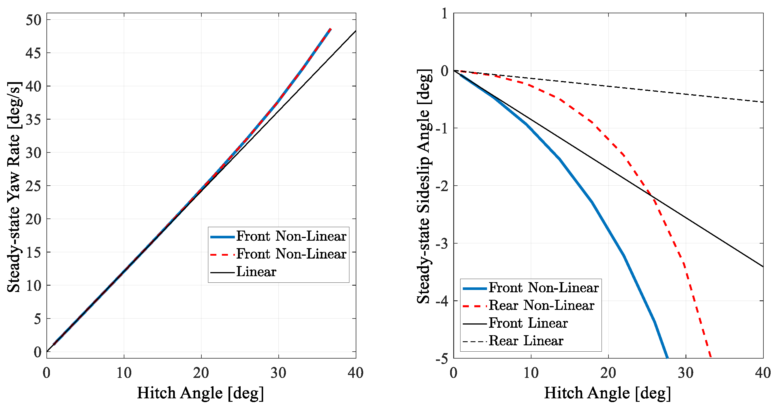
The steady-state response of the linear model was further analyzed by comparing the yaw rate and sideslip angles characteristics with respect to the non-linear model, as reported in Figure 11:
Even if the yaw rate response of the non-linear model is well described by the ATV linearized model for a wider range, the sideslip angles of the front and rear units are only validated for hitch angles lower than 10 deg at a constant speed of 20 km/h. By considering the yaw rate values limited within this range, the liner approximation in Equation (29) is representative of the steady state ATV cornering behavior only for lateral accelerations lower than 1 m/s2.
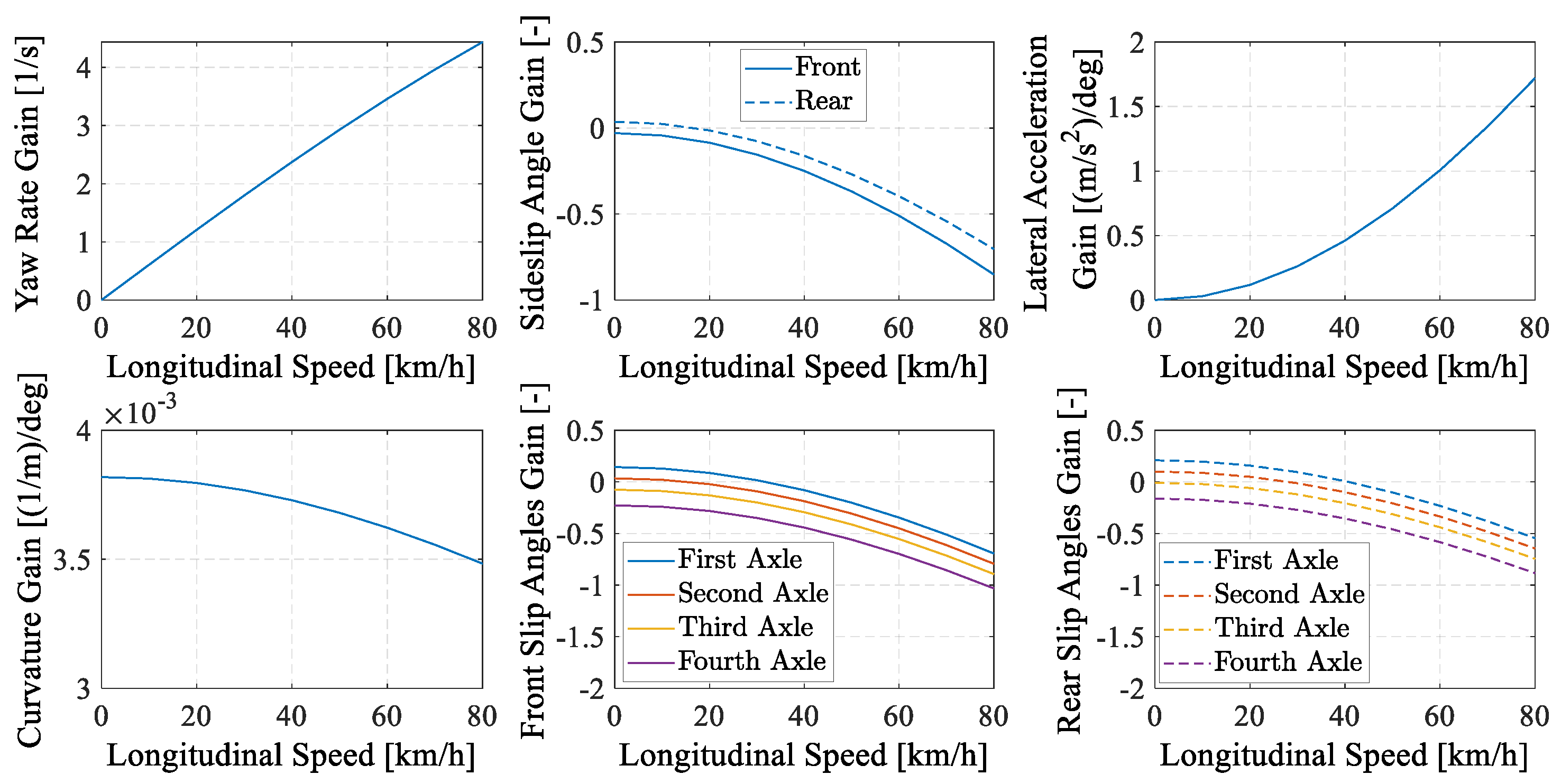
By focusing the analysis within the linear ATV cornering behavior, the influence of the front vehicle speed on steady-state gains, defined in Equation (36), is shown in Figure 12.
The gains evaluated at zero longitudinal speeds represent the “kinematic” ATV steady-state behavior where the effect of inertial forces, due to lateral accelerations, are negligible. The non-null kinematic front and rear slip angle gains show that all the four axles slip on the terrain even at low or zero speed conditions. Moreover, from the curvature gain plot, the ATV shows an evident steady-state understeer behavior: the same value of hitch angle produces a larger curvature radius (inverse of the curvature) and higher front and rear sideslip angles (in module) for higher speeds.
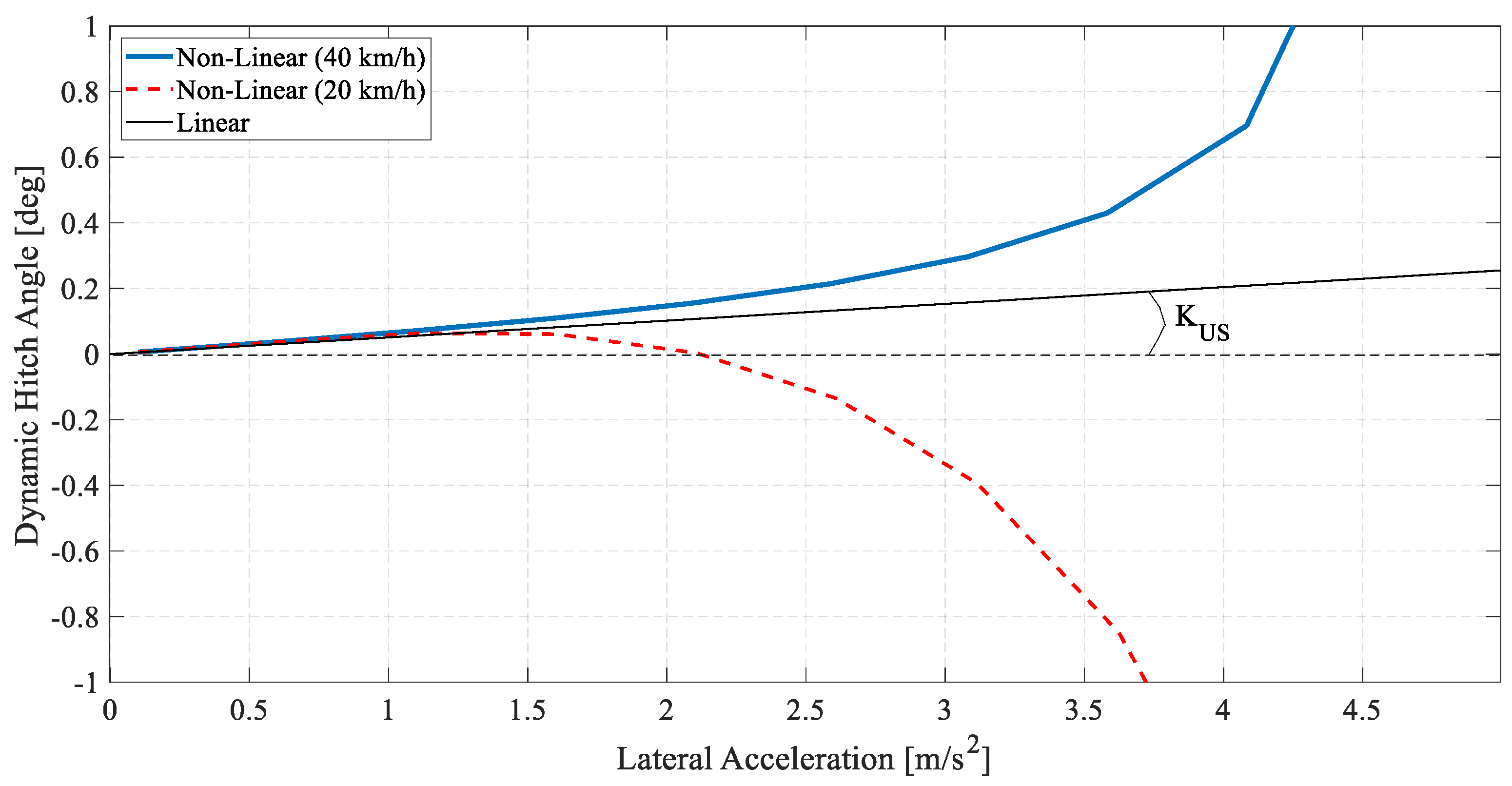
The ATV cornering behavior is also well described by the equivalent understeer characteristics, typical of passenger vehicles. For the ATV, the understeer characteristics represents the dynamic hitch angle correction, with respect to the kinematic condition, required to keep a desired curvature radius for different lateral accelerations. The kinematic hitch angle, , that must be set to follow a desired trajectory at lower speeds (or lateral accelerations) is calculated by considering the kinematic curvature gain :
It must be noted that the single-track model assumptions commonly used for the handling analysis of passenger cars lead to a kinematic gain equal to the inverse of the vehicle wheelbase. On the other hand, the ATV kinematic curvature gain depends on front and rear axle cornering stiffness as well as on vehicle geometrical parameters.
The dynamic hitch angle is then calculated as the difference between the current and the kinematic hitch angles:
The understeer gradient, , is positive for understeering and negative for oversteering ATV behaviors. It can be analytically proved that the understeer gradient of Equation (38) is speed-independent for the linearized model, but the understeering behavior of the non-linear model is strongly influenced by the vehicle speed, especially at higher lateral accelerations, as shown in Figure 13.
In the range of low lateral accelerations ( m/s2), the understeer gradient of the non-linear model is also speed-independent and aligned with the linear model. For higher lateral accelerations ( m/s2), the non-linear model shows a more understeering behavior at 40 km/h and an oversteering behavior at 20 km/h if compared to the linear model. However, the magnitude of the dynamic hitch angle obtained with the non-linear model at high lateral accelerations is not so significant if compared to the absolute hitch angle . For example, at m/s2 the absolute hitch angle obtained with the non-linear model (at km/h) is deg.
4. Hitch Angle Controller
4.1. Controller Design
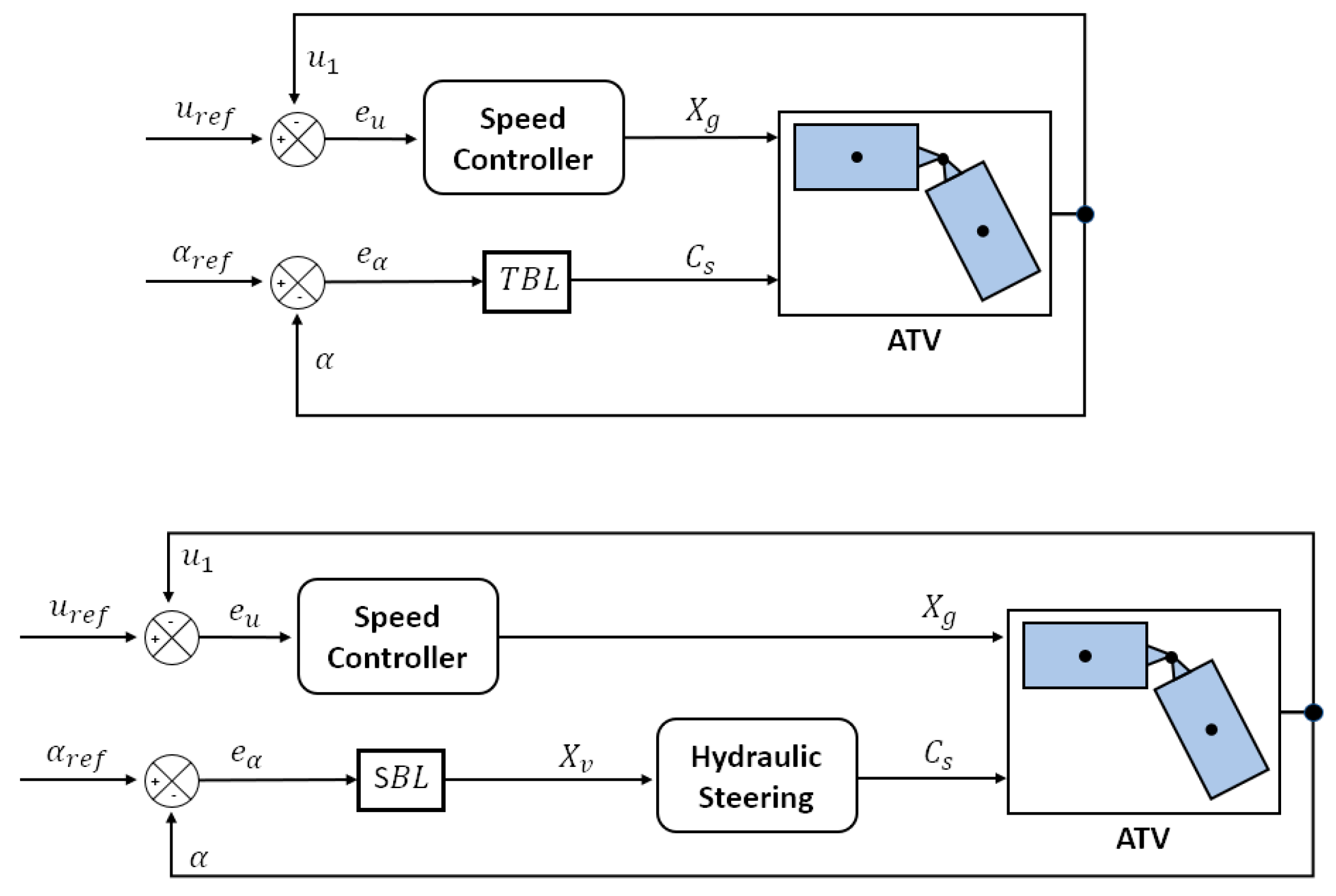
While the previous section analyzed the ATV dynamic behavior through the linearized model, the present section evaluates the influence of the hydraulic actuation system by introducing a hitch angle controller. The hitch angle controller was designed based on the non-linear model, due to the presence of strong nonlinearities that characterize the ATV and the hydraulic pressure dynamics. Two alternatives logics are proposed for controlling the ATV hitch angle, as shown in Figure 14.
Both hitch angle controllers use the error as input for a Proportional Integral Derivative (PID) control logic, where represents the desired hitch angle. One PID logic is designed to elaborate a steering torque , named “Torque-Based Logic” (TBL), and the second PID calculates a hydraulic command valve , named as “Speed-Based Logic” (SBL). In the first case, the hydraulic steering dynamics is excluded by considering an ideal actuator that directly provides the desired steering torque, as assumed for the ATV linearized model and in [22], where an electric motor is directly mounted on the steering joint. For the SBL, the steering torque applied to the ATV depends on the pressure dynamics within the hydraulic circuit of the steering system. The reason behind the selection of these two logics aims at analyzing the impact of a direct steering torque on the ATV lateral dynamics if compared to the steering action applied by the hydraulic circuit, which is influenced by the internal feedback between the actuator and system dynamics. A speed controller is also included in Figure 14 to reduce the speed error by regulating the gas pedal position (not described in this paper). Furthermore, all the feedback signals shown in Figure 14 are assumed to be fully available but feasible estimators are required for practical implementations, as also described in [23]. The two alternative logics are expressed by:
The PID’s gains , , , , and were obtained through the Simulink® “Response Optimization” toolbox. The optimizations process is designed to achieve the desired response to a step input on at a desired ATV speed , kept constant by the speed controller shown in Figure 14, based on the requirements reported in Table 2.
Optimal solution for the set of PID gains depends on the boundary conditions for the optimization problem, such as the ATV speed and the final hitch angle value . An example for optimal PID gains selection is provided in Table 3.
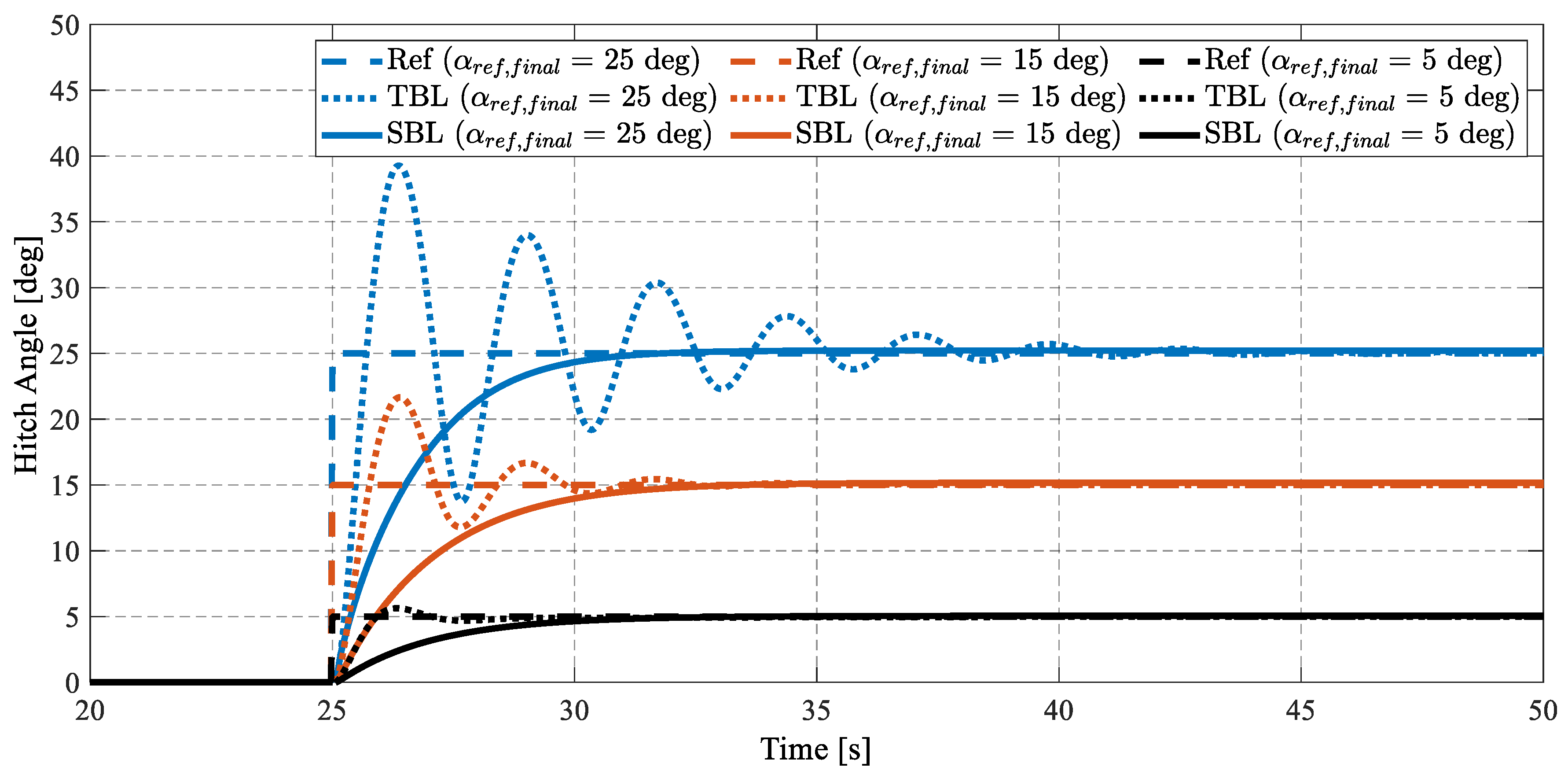
The comparison between the two logics shows that the TBL requires an extreme PID adaptation, in terms of gains magnitude and sign variation, to the maneuver operative conditions. This is mainly due to the strong non-linear characteristics between the steering torque and the hitch angle. On the other hand, the SBL does not require such a drastic PID gains variation since the hydraulic steering circuit automatically adapts the fluid pressure to provide the needed steering torque. This result implies that the SBL structure is more stable than the TBL. A further verification of this concept is represented by the ATV non-linear model response to a step input when a fixed set of PID gains, e.g., the first row in Table 3, is applied for each final hitch angle values. Results are shown in Figure 15.
Even if the PID gains are not adapted for the three operative conditions, the SBL provides a clearly better response if compared to the TBL, which does not respect all the desired performance requirements reported in Table 2, especially in terms of maximum settling time and overshoot. Although the stability of both logics was not assessed through an analytical formulation, the time domain responses described in Figure 15 represent a numerical verification of the controller performance and stability. The SBL shows a more stable response to the reference hitch angle variation with respect to the TBL, which tends to reduce the ATV stability when the amplitude of the reference signal rises, as can be seen by the increase of hitch angle oscillations.
4.2. Controller Validation
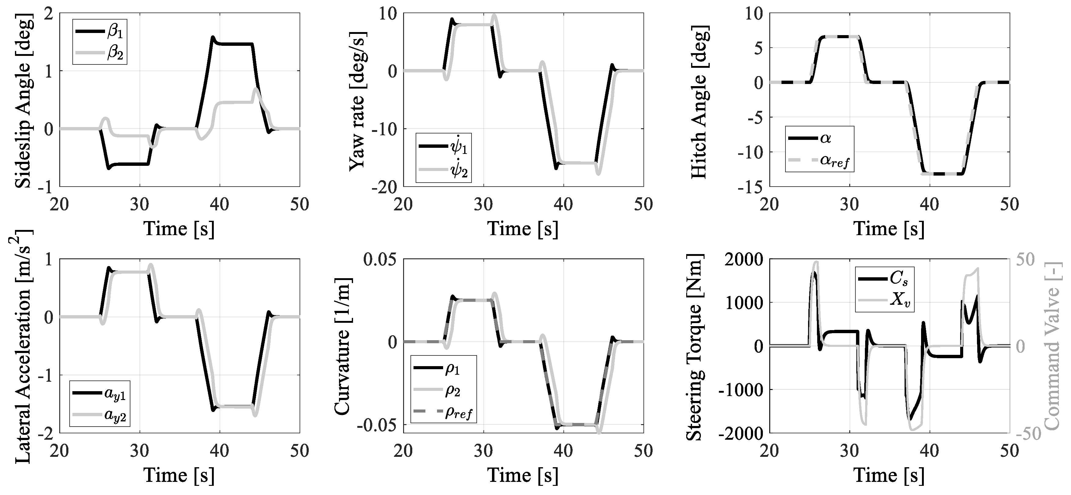
The hitch angle controller with SBL design for deg (first row in Table 3) is then validated through a more realistic multiple turn maneuver. Figure 16 reports the time histories of the main lateral dynamics’ quantities during a multiple turn maneuver at a constant speed of 20 km/h. The simulated maneuver consists of a first swift turn with a curvature radius of 40 m counterclockwise, a second one that brings the ATV on a straight line, a third one with a curvature radius of 20 m clockwise, and a final one that brings back the ATV on a straight line.
The ATV well follows the variable hitch angle required even if a fixed PID gains is adopted for the SBL. It is also remarkable to see that, given the strong non-linear relation between the steering torque and the hitch angle shown in Figure 7, the steering torque required to track the reference hitch angle during a multiple turn maneuver is extremely variable despite the maneuver not being considered as aggressive as proven by the low lateral acceleration condition.
5. Conclusions
The activity presented in this paper describes a non-linear model for a typical ATV and a methodology to linearize the model for the lateral dynamics analysis. The following conclusions are drawn from simulation results:
- The linearized ATV model represents a promising tool for ATV dynamics analysis only in the range of small lateral accelerations ( m/s2).
- The linearized ATV model shows a stable behavior over the whole speed operative range, and it is characterized by a “slow” open-loop dynamics due to the presence of relatively small natural frequencies.
- The steady-state ATV cornering behavior for small lateral accelerations is understeering with the proposed set of vehicle parameters. This is also proven by extending to the ATV the concept behind the understeer characteristics commonly adopted for passenger cars.
- At higher lateral accelerations, the ATV steady-state understeering attitude obtained with the non-linear model is strongly influenced by the vehicle speed. An undesteering behavior is observed for 40 km/h and an oversteering attitude is obtained for 20 km/h.
- The hitch angle controller with SBL represents a better solution if compared to the TBL, since the hydraulic steering circuit automatically adapts the pressure dynamics to the ATV load conditions without any direct steering torque regulation.
Future investigations are necessary to propose a similar methodology to design the hitch angle controller for higher lateral accelerations and in the presence of ATV parameters variation, e.g., the axles’ cornering stiffness. The enhancement of the linearized model represents a fundamental requirement for extending the analytical approach to the hitch angle controller design and its stability and performance assessment as well as its robustness level against uncertain parameters and external disturbances. Moreover, other future developments of this work aim at improving the analytical methodology by including (a) the hydraulic actuation dynamics for enhancing the ATV linearized model accuracy in predicting the ATV lateral behavior, (b) the effect of the ATV track tension on slip angles generation and (c) the modification of the track–terrain contact forces when a soft-soil interaction is required with a non-negligible track sinkage.
Author Contributions
Conceptualization, A.T., E.G. and M.V.; Data curation, A.T.; Formal analysis, A.T.; Methodology, A.T., E.G. and M.V.; Software, A.T.; Supervision, M.V.; Writing—original draft, A.T.; Writing—review & editing, E.G., and M.V. All authors have read and agreed to the published version of the manuscript.
Funding
This research received no external funding.
Conflicts of Interest
The authors declare no conflict of interest.
Appendix A
The aim of this appendix is to provide the non-linear kinematic relation imposed by the steering joint geometry as shown in Figure A1.
The right and left rod displacement, and are evaluated by considering the triangles and :
where , and angle are constant geometric parameters. The speeds of right and left pistons and are obtained by deriving the previous equation:
The hydraulic chamber volumes , and their time derivatives , are then calculated as:
where is the total volume when the ATV is moving in a straight line ().
Finally, the right and left piston force arms and with respect to the steering hinge are calculated by:
Figure A1.
Steering joint kinematics: straight line (blue), turning (red).

References
- Maclaurin, B. A skid steering model with track pad flexibility. J. Terramechanics 2007, 44, 95–110. [Google Scholar] [CrossRef]
- Thai, T.D.; Muro, T. Numerical analysis to predict turning characteristics of rigid suspension tracked vehicle. J. Terramechanics 1999, 36, 183–196. [Google Scholar] [CrossRef]
- Loh, H.F.; Shu, J.; Tu, S.J.; Tay, C.M.; Soon, D.P.Y.; Poon, Y.C.; Leong, H.C. Articulated vehicle, an articulation device and a drive transmission. U.S. Patent No. 6,880,651, 19 April 2005. [Google Scholar]
- Wagner, S.; Nitzsche, G. Rear Carriage Steering Mechanism and Method. U.S. Patent No. 10,336,368, 2 July 2019. [Google Scholar]
- Watanabe, K.; Kitano, M. Study on steerability of articulated tracked vehicles—Part 1. Theoretical and experimental analysis. J. Terramechanics 1986, 23, 69–83. [Google Scholar] [CrossRef]
- Hohl, G.H. Military terrain vehicles. J. Terramechanics 2007, 44, 23–34. [Google Scholar] [CrossRef]
- He, Y.; Khajepour, A.; McPhee, J.; Wang, X. Dynamic modelling and stability analysis of articulated frame steer vehicles. Int. J. Heavy Veh. Syst. 2005, 12, 28–59. [Google Scholar] [CrossRef]
- Rowduru, S.; Kumar, N.; Kumar, A. A critical review on automation of steering mechanism of load haul dump machine. Proc. Inst. Mech. Eng. Part I: J. Syst. Control Eng. 2020, 234, 160–182. [Google Scholar] [CrossRef]
- Pazooki, A.; Rakheja, S.; Cao, D. Kineto-dynamic directional response analysis of an articulated frame steer vehicle. Int. J. Veh. Des. 2014, 65, 1–30. [Google Scholar] [CrossRef]
- Gao, Y.; Shen, Y.; Xu, T.; Zhang, W.; Güvenç, L. Oscillatory yaw motion control for hydraulic power steering articulated vehicles considering the influence of varying bulk modulus. IEEE Trans. Control Syst. Technol. 2018, 27, 1284–1292. [Google Scholar] [CrossRef]
- Tota, A.; Galvagno, E.; Velardocchia, M.; Vigliani, A. Passenger car active braking system: Model and experimental validation (Part I). Proc. Inst. Mech. Eng. Part C: J. Mech. Eng. Sci. 2018, 232, 585–594. [Google Scholar] [CrossRef] [Green Version]
- Galvagno, E.; Tota, A.; Vigliani, A.; Velardocchia, M. Pressure Following Strategy for Conventional Braking Control Applied to a HIL Test Bench. SAE Int. J. Passeng. Cars-Mech. Syst. 2017, 10, 721–727. [Google Scholar] [CrossRef]
- Tota, A.; Galvagno, E.; Velardocchia, M.; Vigliani, A. Passenger car active braking system: Pressure control design and experimental results (part II). Proc. Inst. Mech. Eng. Part C: J. Mech. Eng. Sci. 2018, 232, 786–798. [Google Scholar] [CrossRef] [Green Version]
- Liu, J.Y.; Tan, J.Q.; Mao, E.R.; Song, Z.H.; Zhu, Z.X. Proportional directional valve based automatic steering system for tractors. Front. Inf. Technol. Electron. Eng. 2016, 17, 458–464. [Google Scholar] [CrossRef]
- Ridley, P.; Corke, P. Load haul dump vehicle kinematics and control. J. Dyn. Syst. Meas. Control 2003, 125, 54–59. [Google Scholar] [CrossRef]
- Dong, C.; Cheng, K.; Hu, W.; Yao, Y. Dynamic modelling of the steering performance of an articulated tracked vehicle using shear stress analysis of the soil. Proc. Inst. Mech. Eng. Part D: J. Automob. Eng. 2017, 231, 653–683. [Google Scholar] [CrossRef]
- Yao, Y.; Cheng, K.; Zhang, B.; Lin, J.; Jiang, D.; Gao, Z. A steering model for articulated tracked vehicle considering soil deformation on track–soil interaction. Adv. Mech. Eng. 2018, 10, 1–11. [Google Scholar] [CrossRef] [Green Version]
- Tota, A.; Velardocchia, M.; Rota, E.; Novara, A. Steering Behavior of an Articulated Amphibious All-Terrain Tracked Vehicle. SAE Tech. Pap. 2020. [Google Scholar] [CrossRef]
- Tota, A.; Galvagno, E.; Velardocchia, M.; Rota, E.; Novara, A. Articulated Steering Control for an All-Terrain Tracked Vehicle. In Proceedings of the International Conference of IFToMM ITALY, Naples, Italy, 9–11 September 2020; Springer: Cham, Switzerland, 2020; Volume 91, pp. 823–830. [Google Scholar]
- Cui, D.; Wang, G.; Zhao, H.; Wang, S. Research on a Path-Tracking Control System for Articulated Tracked Vehicles. Stroj. Vestn. J. Mech. Eng. 2020, 66, 311–324. [Google Scholar] [CrossRef]
- Galvagno, E.; Rondinelli, E.; Velardocchia, M. Electro-mechanical transmission modelling for series-hybrid tracked tanks. Int. J. Heavy Veh. Syst. 2012, 19, 256–280. [Google Scholar] [CrossRef] [Green Version]
- Wu, J.; Wang, G.; Zhao, H.; Sun, K. Study on electromechanical performance of steering of the electric articulated tracked vehicles. J. Mech. Sci. Technol. 2019, 33, 3171–3185. [Google Scholar] [CrossRef]
- Guercioni, G.R.; Galvagno, E.; Tota, A.; Vigliani, A.; Zhao, T. Driveline backlash and half-shaft torque estimation for electric powertrains control. SAE Tech. Pap. 2018. [Google Scholar] [CrossRef]
Figure 1.
Simplified schematic of the articulated tracked vehicle (ATV).

Figure 2.
Free body diagram of ATV (top view). Reprinted with permission from ref. [19]. Copyright 2020 Springer Nature Switzerland AG.
Figure 2.
Free body diagram of ATV (top view). Reprinted with permission from ref. [19]. Copyright 2020 Springer Nature Switzerland AG.

Figure 3.
Free body diagram of each track rotational dynamics.

Figure 4.
Simplified schematic of the ATV suspension system.

Figure 5.
Free body diagram of the ATV (front unit view).

Figure 6.
Hydraulic steering circuit 1—Double-acting cylinders; 2—Double-solenoid flow rate proportional valve; 3—Pump; 4—Pressure relief valves; 5—Single-solenoid flow rate proportional valve. Adapted with permission from ref. [19]. Copyright 2020 Springer Nature Switzerland.
Figure 6.
Hydraulic steering circuit 1—Double-acting cylinders; 2—Double-solenoid flow rate proportional valve; 3—Pump; 4—Pressure relief valves; 5—Single-solenoid flow rate proportional valve. Adapted with permission from ref. [19]. Copyright 2020 Springer Nature Switzerland.

Figure 7.
Sideslip angles, yaw rates, steering torque, curvatures, lateral accelerations, and track–terrain yaw moment characteristics from the non-linear model at a constant speed 20 km/h.
Figure 7.
Sideslip angles, yaw rates, steering torque, curvatures, lateral accelerations, and track–terrain yaw moment characteristics from the non-linear model at a constant speed 20 km/h.

Figure 8.
Front (left) and rear (right) unit axle lateral forces (top) and cornering stiffness (down) as a function of slip angles for different values of the lateral acceleration.
Figure 8.
Front (left) and rear (right) unit axle lateral forces (top) and cornering stiffness (down) as a function of slip angles for different values of the lateral acceleration.

Figure 9.
Natural frequencies , damping ratio and poles of the ATV linear model as functions of vehicle longitudinal speed .
Figure 9.
Natural frequencies , damping ratio and poles of the ATV linear model as functions of vehicle longitudinal speed .

Figure 10.
Non-linear (NL) and Linear (L) models response in terms of front () and rear () sideslip angles, hitch angle (), front () and rear () yaw rates for three steering input torques at a constant longitudinal speed km/h.
Figure 10.
Non-linear (NL) and Linear (L) models response in terms of front () and rear () sideslip angles, hitch angle (), front () and rear () yaw rates for three steering input torques at a constant longitudinal speed km/h.

Figure 11.
Steady--state yaw rate, front and rear sideslip angles characteristics for a constant longitudinal speed km/h.
Figure 11.
Steady--state yaw rate, front and rear sideslip angles characteristics for a constant longitudinal speed km/h.

Figure 12.
Steady-state gains of yaw rate (top left), front and rear sideslip angles (top central), front lateral accelerations (top right), curvatures (down left), front slip angles (down central) and rear slip angles (down right) for different front longitudinal speeds.
Figure 12.
Steady-state gains of yaw rate (top left), front and rear sideslip angles (top central), front lateral accelerations (top right), curvatures (down left), front slip angles (down central) and rear slip angles (down right) for different front longitudinal speeds.

Figure 13.
Understeer characteristics for the non-linear model at 40 km/h (blue solid line) and at 20 km/h (red dashed line) and for the linear model (black solid line).
Figure 13.
Understeer characteristics for the non-linear model at 40 km/h (blue solid line) and at 20 km/h (red dashed line) and for the linear model (black solid line).

Figure 14.
Simplified schematic of the Torque-Based Logic (TBL) and Speed-Based Logic (SBL) applied to the ATV non-linear model.
Figure 14.
Simplified schematic of the Torque-Based Logic (TBL) and Speed-Based Logic (SBL) applied to the ATV non-linear model.

Figure 15.
Step response of the non-linear ATV model with TBL and SBL at km/h.

Figure 16.
Sideslip angles, yaw rates, hitch angle, lateral accelerations, curvatures, steering torque, and hydraulic command valve during a multiple turn maneuver, with the hitch angle controller with SBL and fixed PID gains applied to the non-linear model at constant ATV speed 20 km/h. Reprinted with permission from ref. [19]. Copyright 2020 Springer Nature Switzerland AG.


Table 1.
ATV linearized model parameters.
| Quantity | Value | Description |
|---|---|---|
| 3440 kg | Front unit mass | |
| 2440 kg | Rear unit mass | |
| 4472 kg m2 | Front unit moment of inertia around | |
| 3172 kg m2 | Rear unit moment of inertia around | |
| 2.09 m | Front CoG distance from the steering joint | |
| 2.18 m | Rear CoG distance from the steering joint | |
| 0.79 m | Front axle 1 distance from the front CoG | |
| 0.29 m | Front axle 2 distance from the front CoG | |
| −0.21 m | Front axle 3 distance from the front CoG | |
| −0.90 m | Front axle 4 distance from the front CoG | |
| 0.79 m | Rear axle 1 distance from the rear CoG | |
| 0.29 m | Rear axle 2 distance from the rear CoG | |
| −0.21 m | Rear axle 3 distance from the rear CoG | |
| −0.90 m | Rear axle 4 distance from the rear CoG | |
| −0.81 × 10⁵ N/rad | Front axle 1 cornering stiffness 1 | |
| −1.21 × 10⁵ N/rad | Front axle 2 cornering stiffness 1 | |
| −1.28 × 10⁵ N/rad | Front axle 3 cornering stiffness 1 | |
| −0.81 × 10⁵ N/rad | Front axle 4 cornering stiffness 1 | |
| −0.61 × 10⁵ N/rad | Rear axle 1 cornering stiffness 1 | |
| −0.98 × 10⁵ N/rad | Rear axle 2 cornering stiffness 1 | |
| −1.06 × 10⁵ N/rad | Rear axle 3 cornering stiffness 1 | |
| −0.61 × 10⁵ N/rad | Rear axle 4 cornering stiffness 1 |
1 The cornering stiffness is calculated for ( and ).
Table 2.
Desired ATV step response requirements.
| Property | Requirement | Description |
|---|---|---|
| Rise Time | s | Time for the hitch angle to reach the 80% of the step final value |
| Settling Time | s | Time for the hitch angle to settle within a range of 1% around the step final value |
| Overshoot | % | The amount by which the hitch angle can exceed the step final value before settling |
| Undershoot | % | The amount by which the hitch angle can undershoot the step initial value |
Table 3.
Optimal Proportional Integral Derivative (PID) set of gains for different final hitch angles at km/h.
Table 3.
Optimal Proportional Integral Derivative (PID) set of gains for different final hitch angles at km/h.
deg | Nm/rad | Nm/(rad s) | Nm/(rad/s) | 1/rad | 1/(rad s) | 1/(rad/s) |
|---|---|---|---|---|---|---|
| 29093 | 5176 | −1223.5 | 2.0418 | 0.0121 | −0.09323 | |
| 21178 | 2591.5 | 1036.2 | 2.2987 | 0.0131 | −0.1525 | |
| 6345.1 | −265.3351 | 2315.5 | 2.1310 | 0.0119 | −0.1759 |
Publisher’s Note: MDPI stays neutral with regard to jurisdictional claims in published maps and institutional affiliations. |
© 2021 by the authors. Licensee MDPI, Basel, Switzerland. This article is an open access article distributed under the terms and conditions of the Creative Commons Attribution (CC BY) license (http://creativecommons.org/licenses/by/4.0/).
Share and Cite
MDPI and ACS Style
Tota, A.; Galvagno, E.; Velardocchia, M. Analytical Study on the Cornering Behavior of an Articulated Tracked Vehicle. Machines 2021, 9, 38. https://0-doi-org.brum.beds.ac.uk/10.3390/machines9020038
AMA Style
Tota A, Galvagno E, Velardocchia M. Analytical Study on the Cornering Behavior of an Articulated Tracked Vehicle. Machines. 2021; 9(2):38. https://0-doi-org.brum.beds.ac.uk/10.3390/machines9020038
Chicago/Turabian StyleTota, Antonio, Enrico Galvagno, and Mauro Velardocchia. 2021. "Analytical Study on the Cornering Behavior of an Articulated Tracked Vehicle" Machines 9, no. 2: 38. https://0-doi-org.brum.beds.ac.uk/10.3390/machines9020038
Note that from the first issue of 2016, this journal uses article numbers instead of page numbers. See further details here.