
VIAM-USV2000: An Unmanned Surface Vessel with Novel Autonomous Capabilities in Confined Riverine Environments


1
Department of Control & Automation, Faculty of Electrical & Electronics Engineering, Ho Chi Minh City University of Technology (HCMUT), 268 Ly Thuong Kiet Street, District 10, Ho Chi Minh City 754000, Vietnam
2
Vietnam National University Ho Chi Minh City, Linh Trung Ward, Thu Duc District, Ho Chi Minh City 754000, Vietnam
3
Department of Mechanical Engineering, Korea Maritime and Ocean University, Busan 49112, Korea
4
Interdisciplinary Major of Ocean Renewable Energy Engineering, Korea Maritime and Ocean University, Busan 49112, Korea
*
Author to whom correspondence should be addressed.
Machines 2021, 9(7), 133; https://0-doi-org.brum.beds.ac.uk/10.3390/machines9070133
Submission received: 29 May 2021
/
Revised: 5 July 2021
/
Accepted: 8 July 2021
/
Published: 15 July 2021
(This article belongs to the Special Issue Dynamics and Motion Control of Unmanned Aerial/Underwater Vehicles)
Abstract
:Unmanned Surface Vessels (USVs) have witnessed an increasing growth in demand for development due to their compactness, mobility and maneuverability, which make them well-suited for environmental monitoring on narrow water in Vietnam in particular and in general at several similar tropical regions. However, current surface vessels are limited to operation on open water only. In this paper, we design a USV, namely, VIAM-USV2000, equipped with advanced autonomous capabilities to satisfactorily carry out missions in confined riverine environments. More specifically, our prototype is designed to follow a smooth B-Spline path that is self-planned to meet the limiting curvature and avoid static obstacles. Moreover, the vessel is capable of avoiding dynamic obstacles by an advanced Set-based Guidance mechanism. Simulated and experimental results at a local lake prove the effectiveness of the proposed capabilities, thereby paving the way for the extensive deployment of USVs in many real-world applications.
1. Introduction
The growing demand for water-based environmental monitoring, resource exploiting and hydrology surveying leads to an increasing interest in the development of innovative unmanned surface vessels [1,2,3]. In particular, USV shows enormous potential in leveraging the task of monitoring water quality at canals and narrow rivers due to its high compactness, mobility and maneuverability, thereby reducing the operating cost to a minimum.
In recent decades, several USV prototypes have been introduced [4,5], all of which are developed for open-sea operation, thus not satisfying the autonomous requirements in confined, complicated and dynamic environments. This fact is particularly held in the case of Vietnam and many tropical regions, making water sampling and monitoring tasks in those areas extremely difficult. Recently, some new prototypes such as Roboat [6] and Roboat II [7] succeed in maneuvering through narrow and crowded urban waterways for transportation of goods and passengers. This helps encourage USV to be more extensively deployed in other restricted regions such as riverine ones.
This paper focuses on designing an unmanned surface vessel, namely, VIAM-USV2000, that inherits and enhances the mechanical and electrical design of VIAM-USV1000 [8]. USV2000 differs from its predecessor in its advanced autonomous capabilities: generate and follow a smooth parameterized curve, avoid dynamic obstacles. For path planning, on the grounds of our former results [9], the B-Spline path [10] is used, and its shape is optimized by a genetic algorithm [11] to meet the limiting curvature. We make an improvement to this path planner so that it can avoid static obstacles. In comparison with other path-generating schemes such as rapidly exploring random trees [12] and Dubins paths [13], B-Spline curves possess several notable advantages, some of which are multi-degree smoothness and local deformation when altering waypoints, thus being suitable for planning collision-free paths through restricted areas. To diminish overshoot when changing waypoints in straight Line-of-Sight (LOS) path following [14], a continuous LOS law for tracking curves is proposed, which features an iterative approach to find the projection of the vessel’s center of navigation onto the curve by Newton–Raphson method.
During navigation of USV, sudden encounters with dynamic obstacles are unavoidable. To avoid these, while Dynamic Window Approach [15] and Vector Field Histogram [16] depend on the vehicle’s dynamics, Velocity Obstacle (VO) [17] presents a study on the accuracy of estimated distance and relative velocity to each obstacle to determine an efficient, local, collision-free path. As a result, by utilizing VO, USV is not only able to easily avoid multiple obstacles from different directions, but it can also return to the global path quickly. Another benefit of VO comes from integration with COLOREGS law [18] and straight LOS law to achieve an obstacle avoidance mechanism, namely, Set-based Guidance (SBG) [19]. In this paper, an advanced SBG law that generates a collision-free trapezium-like local path is proposed for the vessel to maintain a safe distance with each obstacle more easily. We further complement our simulated results in [20] with experimental ones, using USV2000 as the main surface vessel in different avoiding scenarios.
Our main contributions in this paper can be summarized as follows:
- Design hardware-related and software-related components for an unmanned surface vessel, namely, USV2000, to realize advanced autonomous capabilities in confined riverine environments.
- Enhance the B-Spline path planner so that it can automatically optimize the curve’s shape to meet the limiting curvature and avoid static obstacles.
- Develop a continuous LOS path follower for USV to smoothly follow any arbitrary parameterized curve.
- Develop an advanced SBG law that generates a trapezium-like path for the vessel to avoid dynamic obstacles.
- Provide extensive simulated and experimental results to verify the effectiveness of the proposed algorithms in USV2000.
This paper is structured as follows: Section 2 gives a brief overview of hardware specifications and software components, Section 3 gives a detailed description of the path planner, Section 4 explains the path follower in detail, Section 5 illustrates how the obstacle avoider works, Section 6 presents simulated and experimental results and Section 7 concludes the paper.
2. System Development
2.1. Hardware Construction
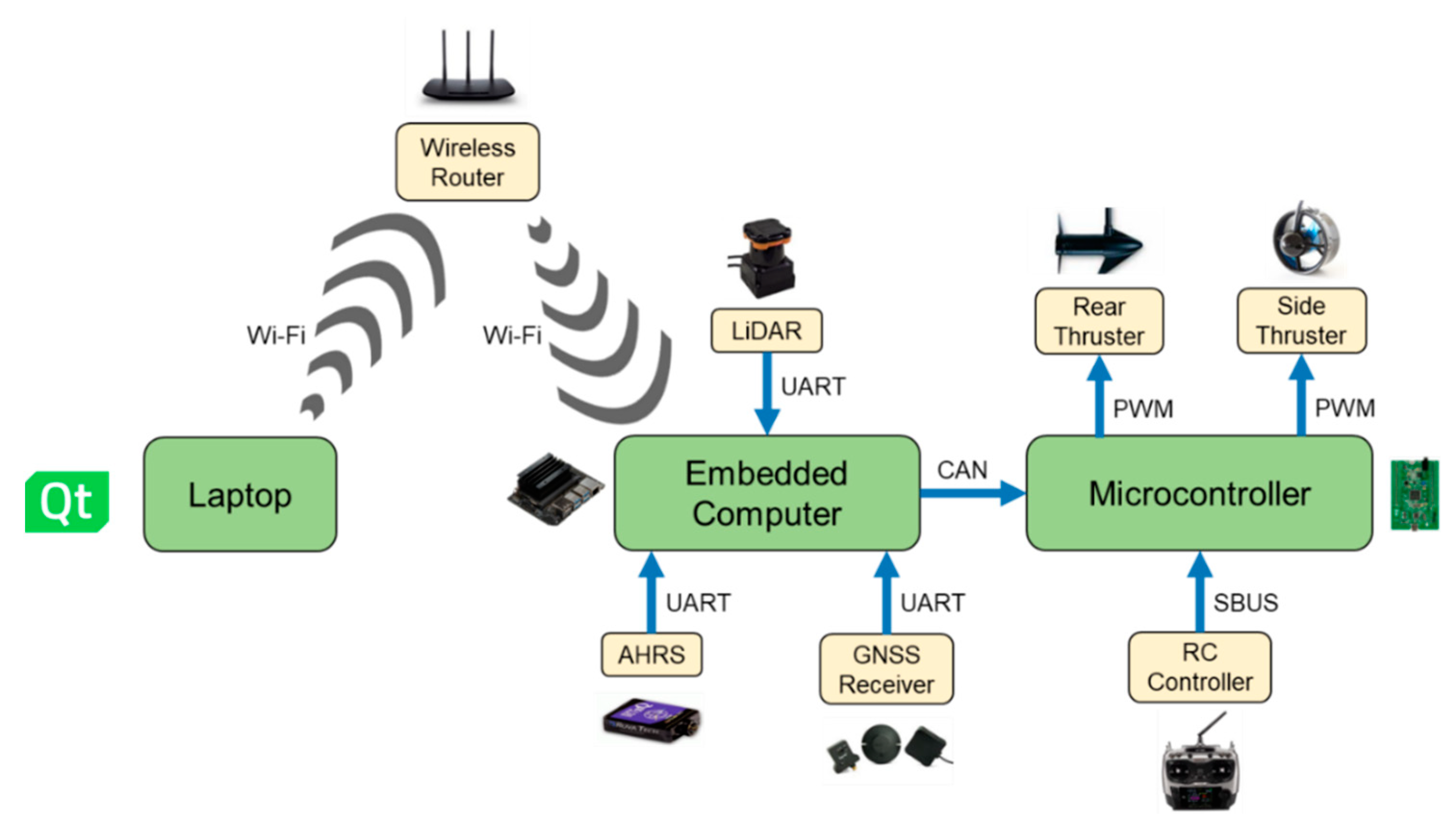
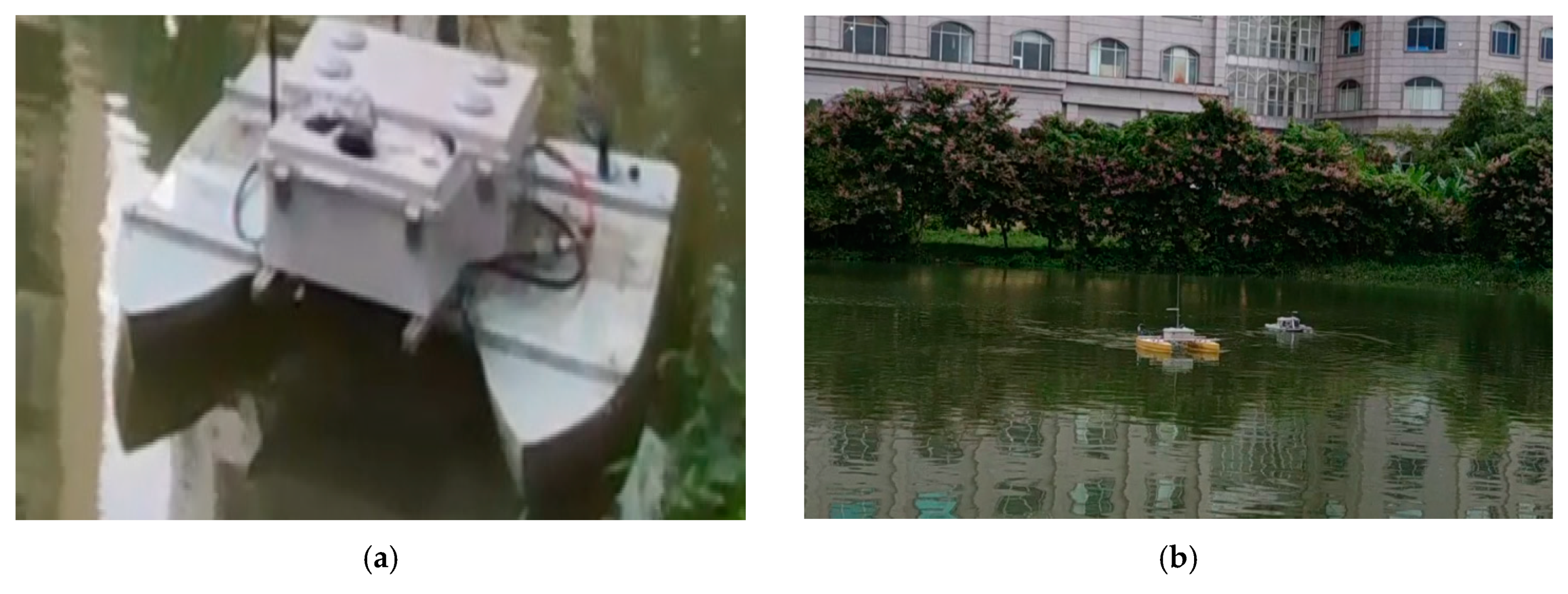
USV2000 features a catamaran design (Figure 1). As shown in Figure 2, the vessel’s actuators are composed of two rear thrusters for moving forward and two side ones for turning. A microcontroller is used to control these thrusters by exporting PWM signals and receive commands from a remote RC controller. An embedded computer plays a central role in realizing navigation, guidance and control strategies: each software component is modularized and exchanges messages in Robot Operating System (ROS) ecosystem. GNSS receiver, AHRS and LiDAR communicate with an embedded computer through UART interface. Data interchange of the embedded computer with a microcontroller is realized by CAN bus, with laptop by Wi-Fi protocol. Detail about each hardware component is mentioned in Table 1.
2.2. Software Composition
As in Figure 3, the vessel’s autopilot software suite in embedded computer, namely, VIAM-USV-VC, for USV2000 is composed of components that are modularized on the ground of the ROS platform. Each software is organized into a task-specific C++ ROS node that communicates with one another via TCPROS protocol. While Navigator publishes the vessel’s pose from GNSS receiver’s and AHRS’s data, Guider realizes a variety of guidance modes (straight-line path following, curve path following, SBG obstacle avoidance) and Controller exports PWM signal for each side thruster based on the current heading error. In addition, LiDAR Transceiver, STM Transceiver and GCS Transceiver are in charge of converting from packets of ROS-exterior protocols (UART, CAN, MAVLink) to that of ROS-interior ones (TCPROS). To maximize resource usage efficiency, we utilize two types of TCPROS connection: message (periodic update by a publish–subscribe mechanism) and service (temporarily available on demand by a request–respond mechanism).
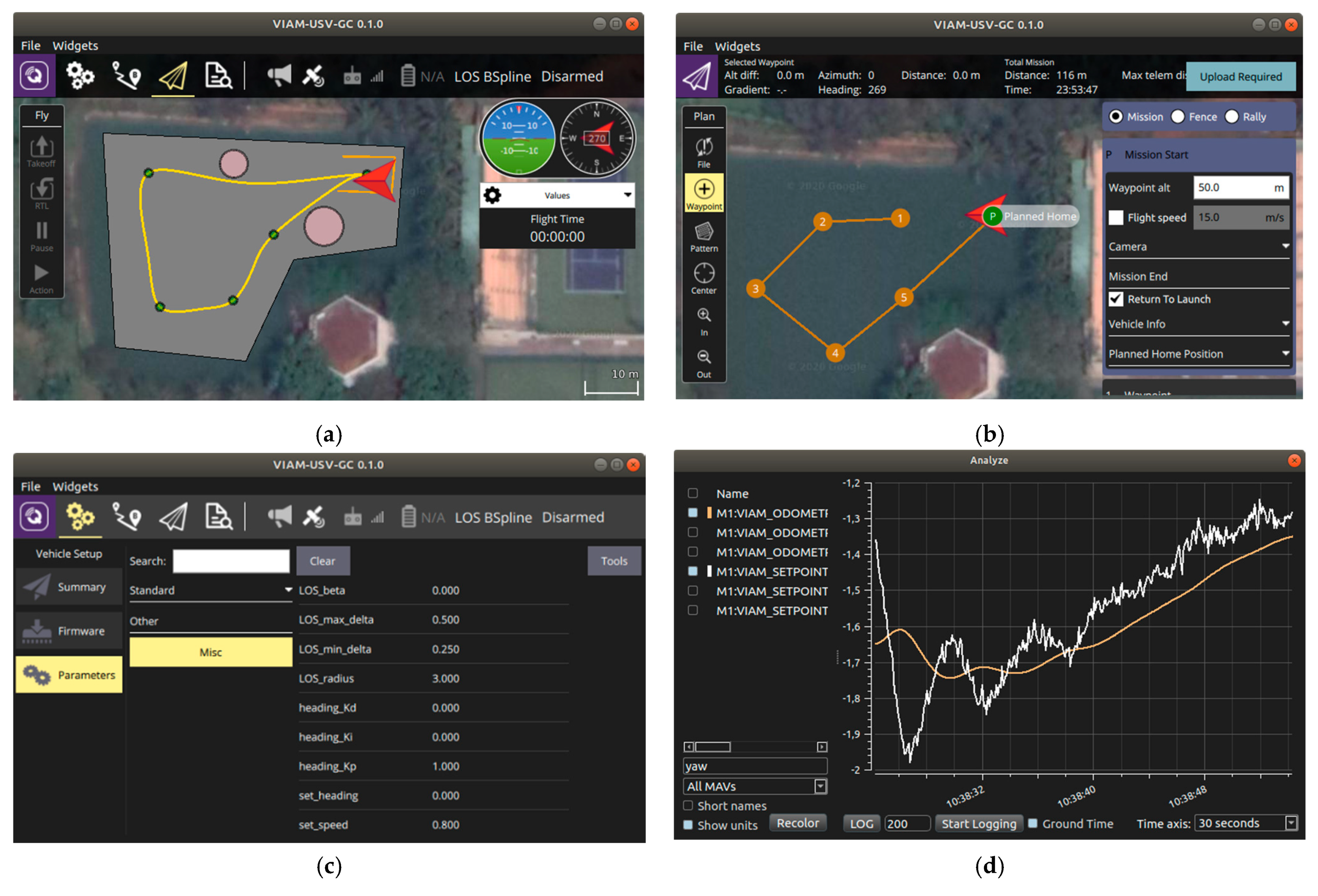
The vessel’s ground control station (GCS) (Figure 4), namely, VIAM-USV-GC, is a highly customized version of QGroundControl that features two programming layers: QML and C++. QML deals with the front-end part of GCS, offering user-friendly interaction via images, sound, notifications, data visualization, data plotting, etc. On the other hand, C++ makes up the back-end part of GCS, handling computer-intensive tasks such as database management, memory management, device drivers and threading. MAVLink is used to facilitate an efficient, reliable and remote data interchange between ROS-based autopilot and GCS for several advantages: tiny packet’s length (max. 279 bytes); support for detecting packet drops, corruption and packet authentication; cross-platform compatibility.
3. Path Planning
3.1. B-Spline Path Generation
B-Spline [10] is a combination of polynomial curves with a degree that goes through a set of pre-defined waypoints . It is parameterized by a variable as follows:
where is the position vector at every curve’s point, is the control vector and is the normalized basis polynomial of a degree. Value of at every is recursively calculated by the following formula [10]:
Control vectors are derived from the solution of the following equation:
where an intermediate variable for every waypoint is selected by the centripetal method [21].
From our observation, if the initial heading of the vessel is not taken into account, the generated B-Spline path may contain sharp turns that make it difficult for the vessel to track. Therefore, as in [22], we constrain the path to the desired initial and final velocity vectors of the vessel, denoted and , respectively, and extend by two more equations as follows:
3.2. Genetic Algorithm for Optimal B-Spline Shaping
To adjust the curvature and avoid obstacles, we generate an additional waypoint between initially assigned ones and optimize their positions for minimum path length using a genetic algorithm (GA). Our method takes advantage of the B-Spline’s locality: the shape of a B-Spline curve is only locally affected when adding, removing or altering waypoints. This property also helps boost the convergence rate when a heuristic search is performed to optimize the curve’s shape.
GA [11] is a popular search-based technique for finding optimal or near-optimal solutions to multi-objective problems. Inspired by biological mechanisms such as mutation, crossover and selection, GA is particularly suited for path planning because of its efficiency when the search space is large and a large number of parameters is involved. In GA, each possible solution is termed an individual, and each search space at every iteration is called a population. By selectively performing crossover across members of the parental population, the descent one is expected to produce a higher number of fitter individuals, or in other words, solutions that are nearer to the optimum. In addition, mutation is employed to maintain genetic diversity from one generation to the next.
Similar to [9], every individual in a population is encoded as follows:
where is the added waypoint to reshape the curve and and are the initial and final velocity vectors.
To create the initial population, every added waypoint is randomly selected in a square region formed by two nearby original waypoints. Panmictic generalized intermediate recombination [23] is used for crossover. Inspired by [24], the cost function to evaluate each individual’s fitness is as follows:
where represents the path’s length associated with each individual , is the maximum path’s length in the current population and is the total penalty function as follows:
If all individuals satisfy constraints, only depends on the path’s length. Otherwise, depends on both the path’s length and penalty function. The philosophy behind this cost function’s design is to favor satisfying all constraints, which includes curvature limiting and obstacle avoidance to search for the shortest path.
After finding the vessel’s radius of turning through maneuvering test, the limiting curvature is defined as:
The penalty component of curvature is calculated using and the maximum curvature of the curve associated with each individual :
where of a parameterized curve is calculated as follows:
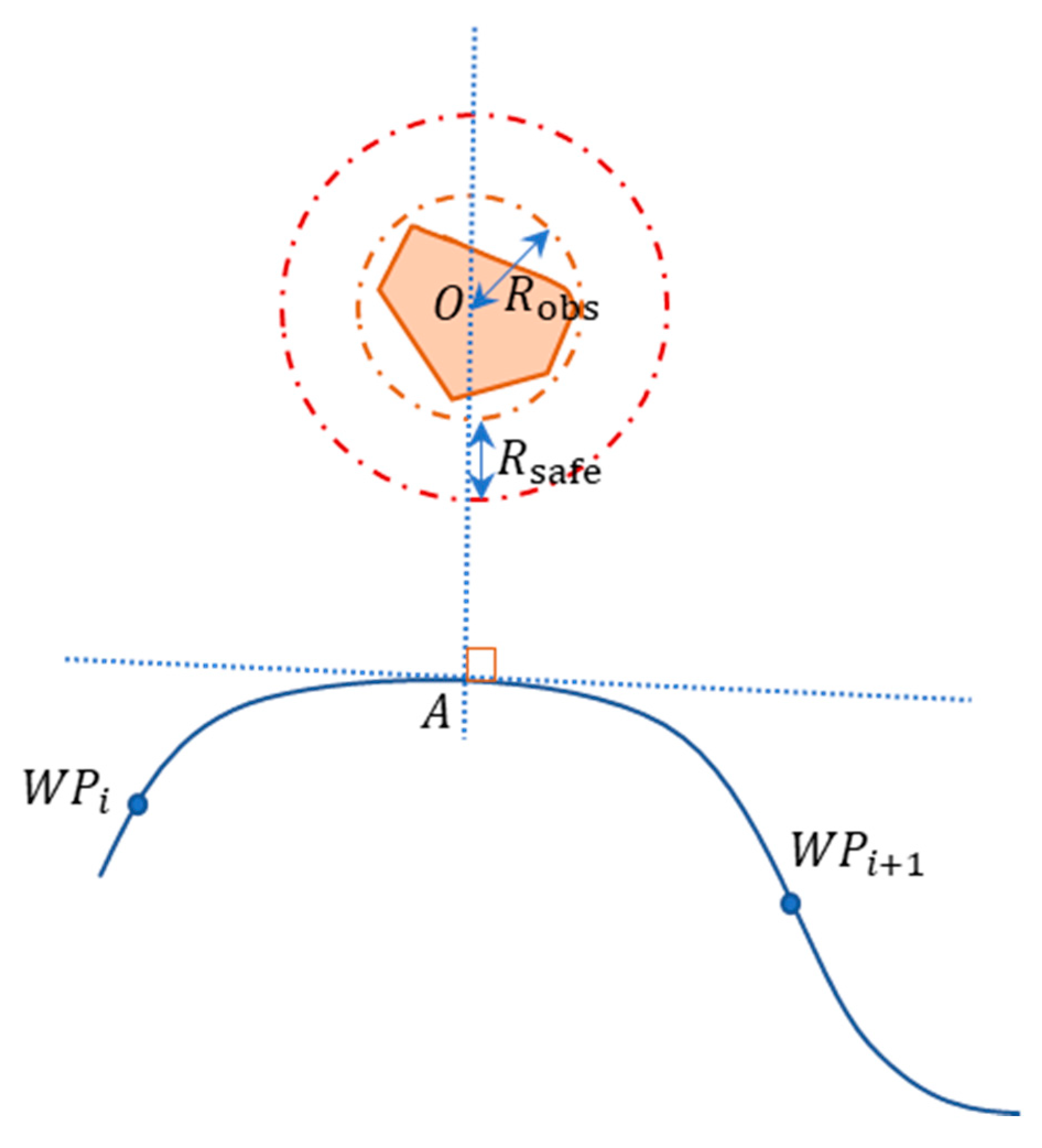
To plan a collision-free path through static obstacles, we complement our former path planner [9] with an additional penalty term in that punishes the act of obstacle collision. Consider an obstacle i with center in Figure 5:
The radius of avoidance is the summation of the obstacle’s radius and radius of safety :
For efficiency, instead of a brute-force search at every point on the curve for , we limit the searching region between two nearest original waypoints from . Then , which is the projection of onto the curve, can be found by an iterative procedure based on Newton–Raphson method in Section 4. After is found, we obtain and compare with to arrive at the penalty component relating to obstacle :
4. Path Following
Given a smooth parameterized curve as follows:
Our task is to design a law that makes the vessel follow this curve as close as possible. As in Figure 6, instead of discretizing the curve and applying straight LOS law among infinitesimal displacements, we devise a new method to track the curve by first finding the projection of the vessel’s center of navigation .
Then cross-track error (CTE) is calculated based on coordinates of the projection , coordinates of the vessel and the tangent angle :
where is continuously computed by trigonometric relation between partial derivatives:
Finally, the desired heading sent to the controller is as follows:
where determines how quickly the vessel returns to the path. If is set too high, the vessel returns quickly but can oscillate.
To find , we apply the Newton–Raphson iterative method. Our new scheme to find the projection is as follows in Table 2:
5. Obstacle Avoidance
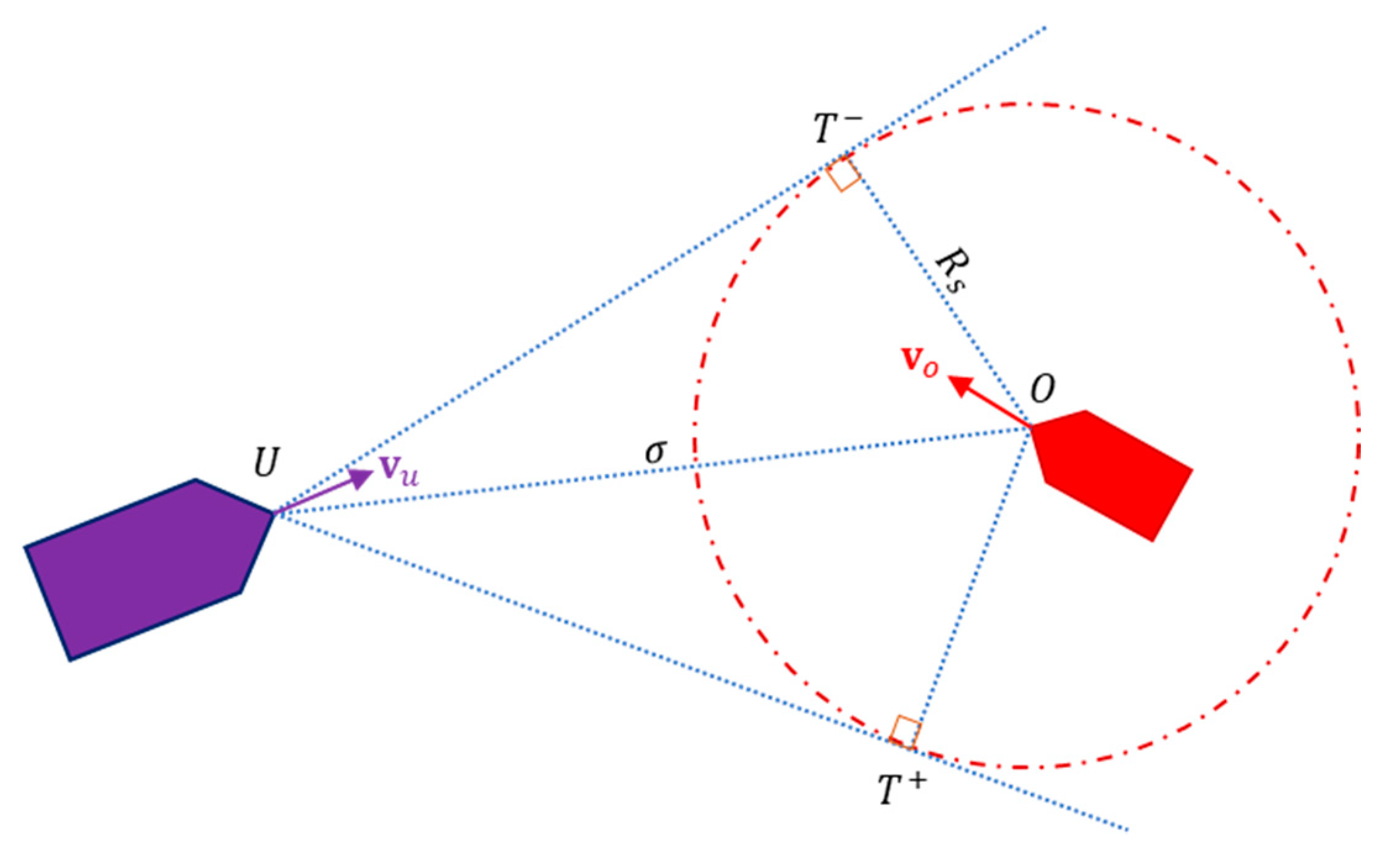
According to Velocity Obstacle (VO) algorithm (Figure 7), in the obstacle’s frame of reference, the obstacle can be considered static and the vessel moves with a relative velocity , so we can simplify a dynamic obstacle avoidance problem into a static one.
An obstacle is modeled by a single point with a radius of danger . The region bounded by the polygon is denoted . When , anchored in the vessel, lies within , it may collide. So to prevent collision, must satisfy:
where is the relative displacement between the vessel and obstacle. Upon obstacle detection, the vessel must change direction so that the new relative velocity satisfies . This is realized by making collide with or according to COLOREGS law in Table 3, where is the current heading of the obstacle.
The final desired heading that the vessel must drive towards is as follows:
where and is the desired velocity of the vessel.
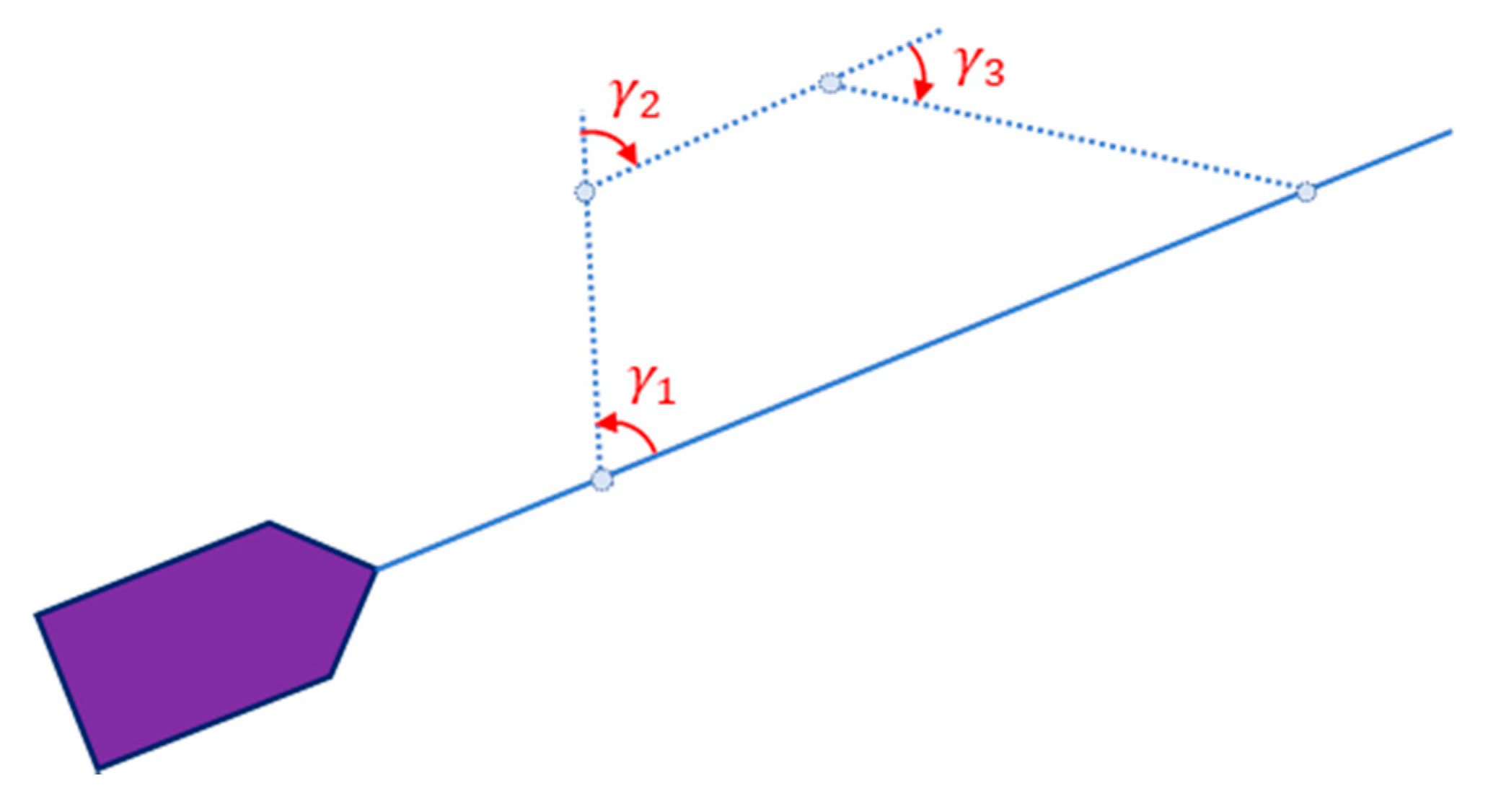
Advanced SBG (Figure 8) enhances the performance of SBG with four distinct modes: tracking (mode 1), avoiding (mode 2), distance keeping (mode 3) and homing (mode 4). Within modes 2–4, the vessel is commanded to track every trapezoid’s side with desired headings auto-selected from VO to efficiently and safely avoid obstacles.
To realize the advanced SBG, we need to find , and as follows:
where is the slope of the global path, in case of head-on and in case of overtaking and crossing, is the moment to enter mode 2 when the distance between our vessel and the obstacle drops below a threshold. The moment to enter mode 3 and mode 4 is when meets but with the assumption that equals and , respectively.
6. Simulated and Experimental Results
To verify the effectiveness of the proposed algorithms, we carry out computer simulations in MATLAB and experiments in a local lake. The B-Spline path planner is firstly implemented in MATLAB for ease of design and evaluation, then realized by C++ code in VIAM-USV-GC to facilitate user-friendly interaction. The continuous LOS path follower is validated by simulated MATLAB results before C++ realization in VIAM-USV-VC for experiments. We only provide experimental results of our advanced SBG scheme since simulated ones are extensively discussed in [20].
6.1. Simulated Result of B-Spline Path Planner and Continuous LOS Path Follower
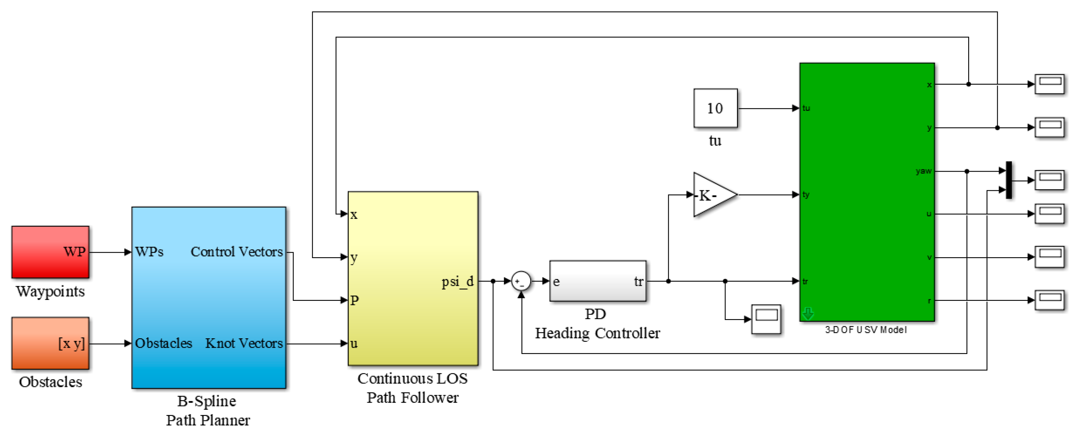
As in Figure 9, we build a MATLAB/Simulink system to simulate the behavior of B-Spline path planner and continuous LOS path follower before real-world deployment. A PD heading controller is implemented to generate heading torque for a reduced 3-DOF USV model.
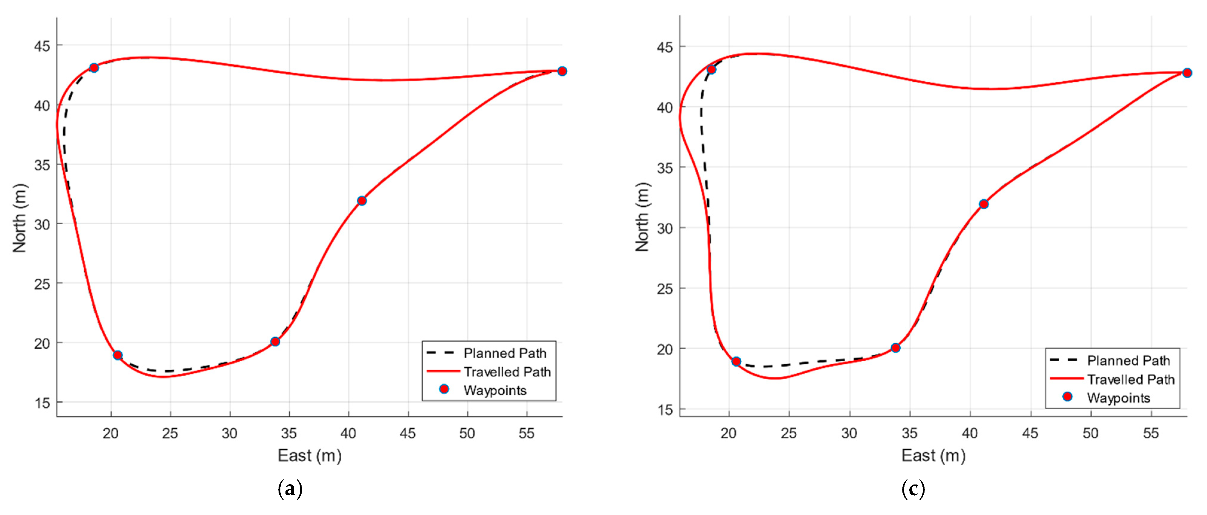
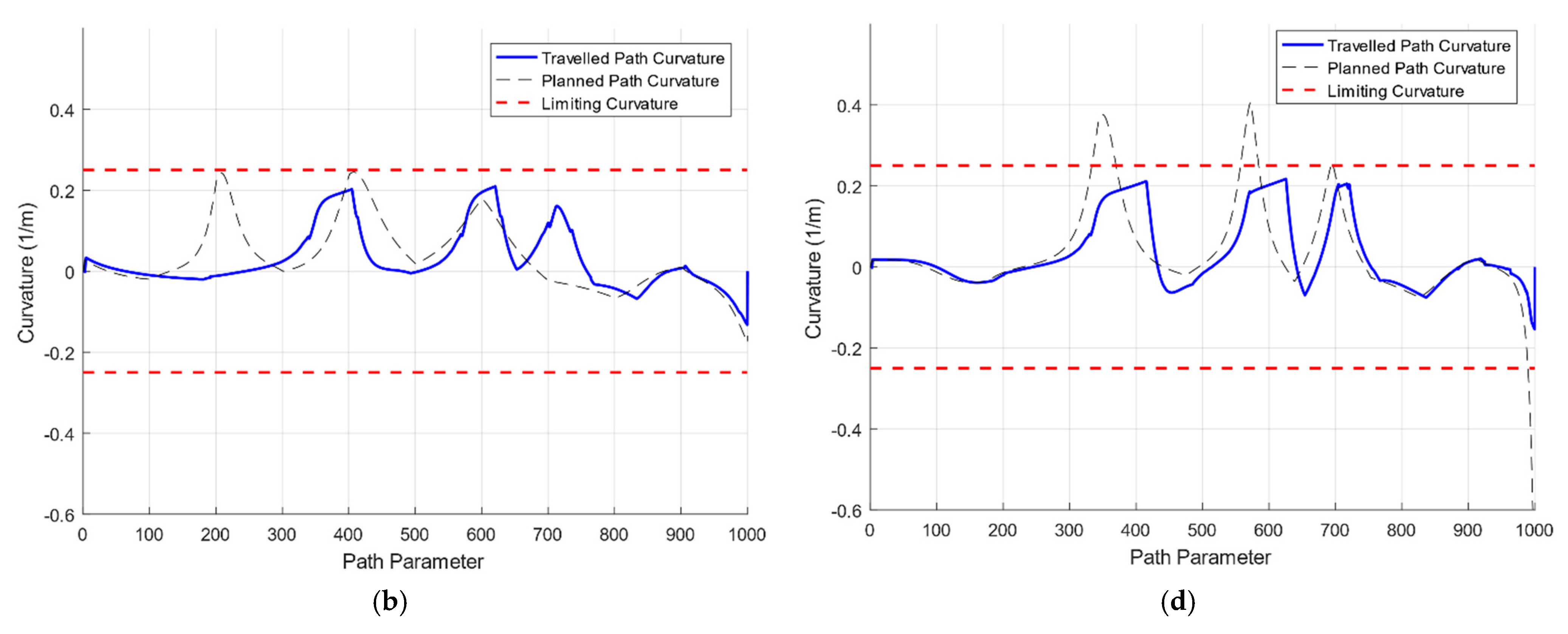
It is essential that the vessel go past every waypoint. To accomplish this mission, we examine how the vessel’s physical turning capability affects the tracking performance by planning two paths, one satisfying (case 1) the limiting curvature and the other not (case 2) (Figure 10).
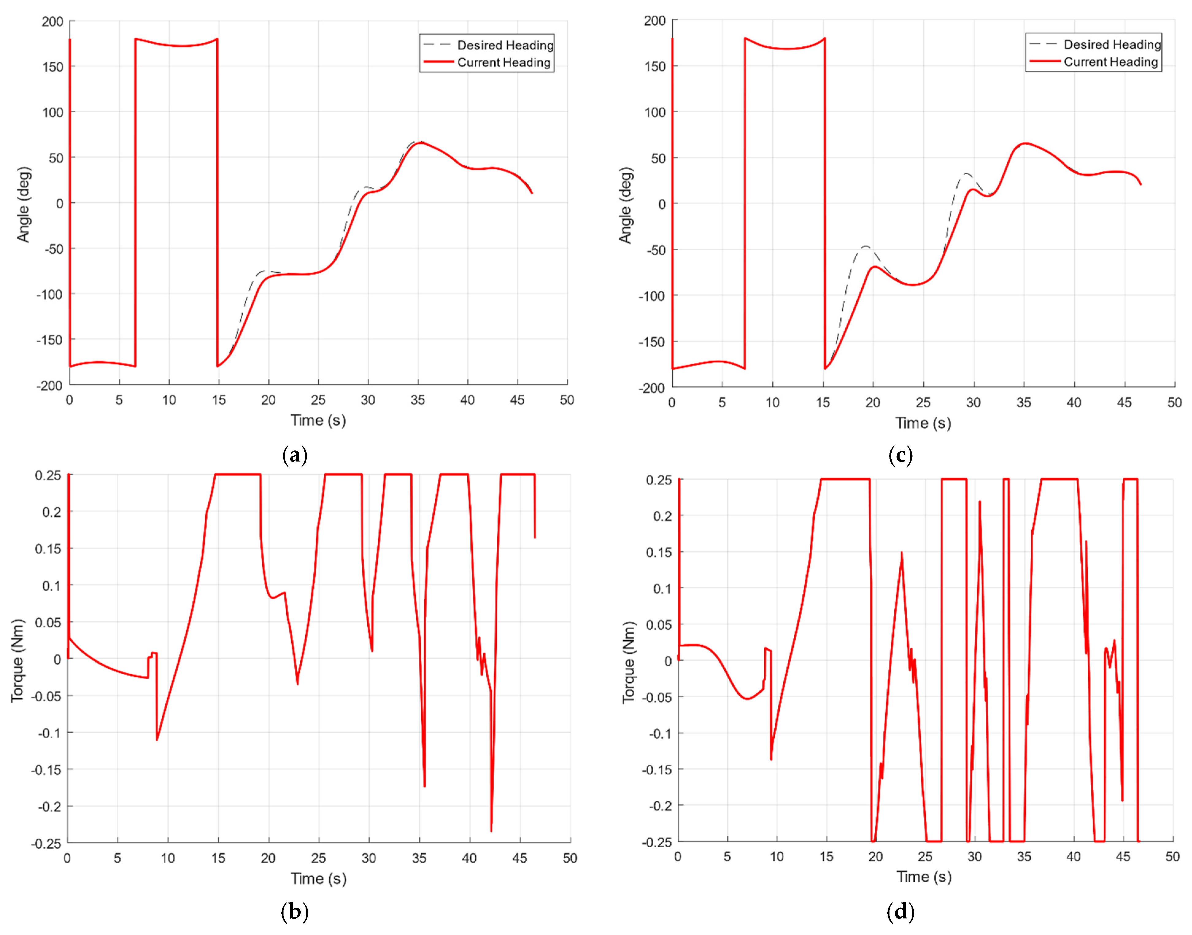
Figure 11 and Table 4 imply that although the length of the planned path in case 2 is shorter than that of case 1; the traveled distance is longer since the vessel cannot physically follow this path. In terms of heading tracking, according to Figure 12 and Table 4, the heading error in case 1 is smaller than that of case 2, resulting in the control signal in case 1 fluctuating less. This makes CTE in case 1 significantly smaller compared to that of case 2. Finally, the original objective to go past waypoints in case 1 is accomplished to a greater extent. A conclusion worth drawing from this simulated result is that designing a path that meets the limiting curvature plays an essential role in excelling the path following’s performance in general.
6.2. Maneuvering Test
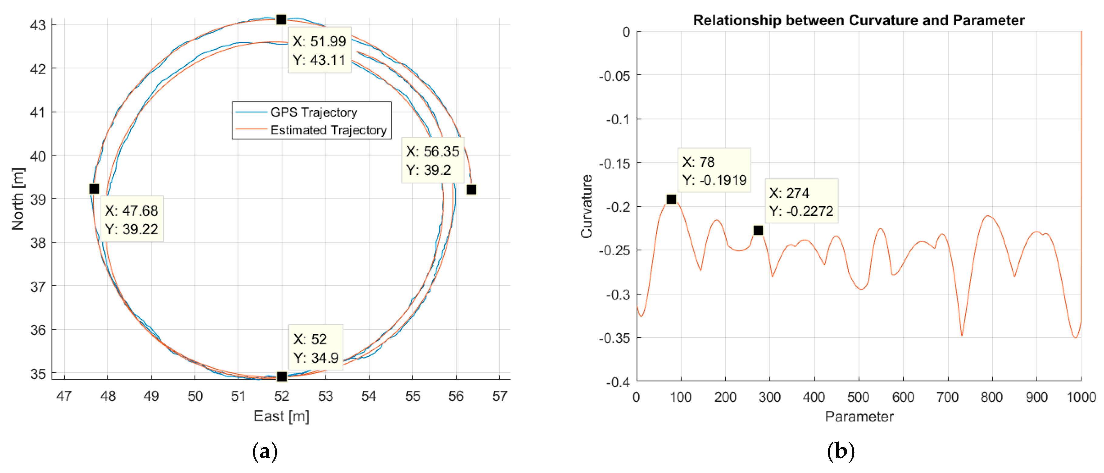
The purpose of this test is to determine the USV2000′s radius of turning, whose inversion is the limiting curvature of the vessel. The procedure is as follows: we export a fixed PWM signal (40%) to two rear thrusters but a maximum (100%) PWM signal to two side ones. Given that the obtained GPS position is very noisy, approximate B-Spline interpolation [22] is chosen to interpolate a smooth parameterized curve from noisy GPS data in order to calculate the curvature at every point on the traveled trajectory. As in Figure 13, it is apparent that the estimated trajectory is very smooth and fits quite well with the original GPS one.
From this estimated B-Spline path, we can easily plot the curvature at every point (Figure 13) and pick the suitable curvature (Table 5) as a candidate for the calculation of the radius of turning. From now on, USV2000′s radius of turning is chosen as 4 m, resulting in the limiting curvature being 0.25 m−1.
6.3. Experimental Result of B-Spline Path Planner and Continuous LOS Path Follower
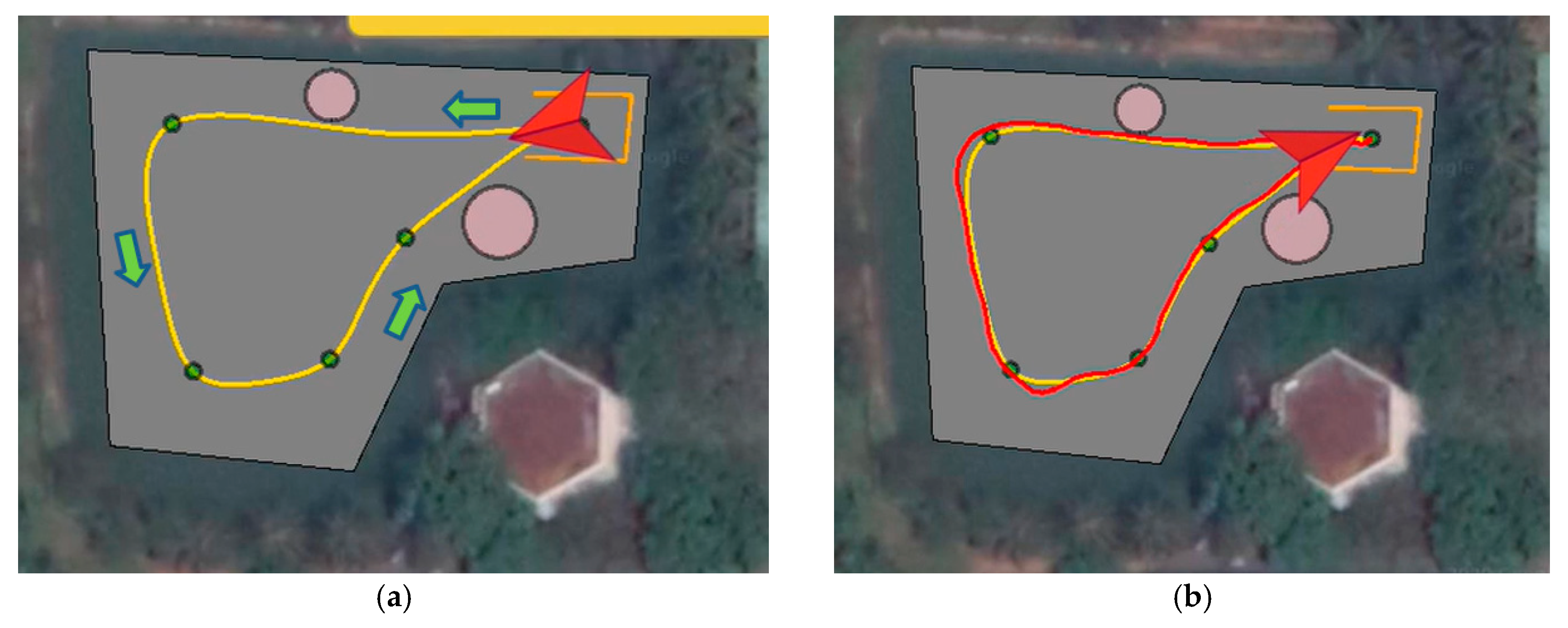
In this experiment, we design a mission as follows: first, USV2000 departs from a harbor with a minus-90-degree heading, then follows the planned path as close as possible and finally returns home with a 90-degree heading. The environment that our vessel must operate is a local lake, which is confined in space and small in size. This poses a huge challenge to vessels, since they can accidentally collide with the bank when making a sharp turn. This type of collision is uncontrollable and mainly stems from the fact that our vessel cannot physically follow those paths whose maximum curvature exceeds the vessel’s limiting one. To solve the problem, our proposed path planner comes into play. Parameters of B-Spline path planner with GA optimization are listed in Table 6. As can be seen in Figure 14, the planned B-Spline path not only goes through all waypoints and avoids static obstacles but also meets the limiting curvature of USV2000 (Figure 15).
After path planning, the vessel needs to follow the pre-defined path as close as possible. A PD heading controller is implemented, and a constant PWM signal (40%) is exported to two rear thrusters. As in Figure 14, the fitness between the traveled and planned paths is acceptable in relation to the overall traveled distance. From Table 7 and Figure 16, it is noticeable that the heading error is quite small, resulting in the control signal exhibiting a slight fluctuation in amplitude. Our vessel tracks well through all waypoints with a maximum deviation of 0.47 m and does not violate prohibited regions.
6.4. Experimental Result of Advanced SBG for Obstacle Avoidance
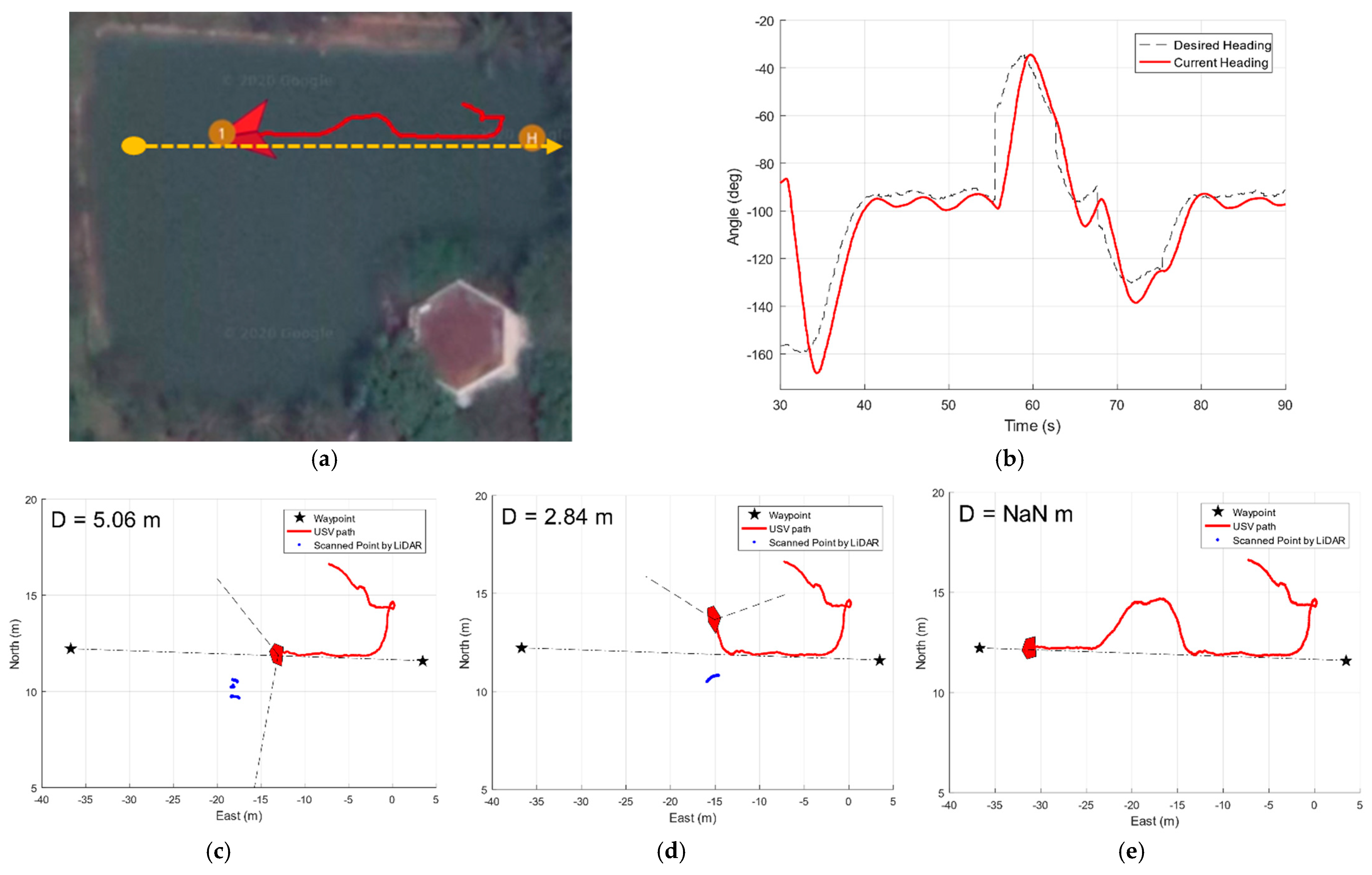
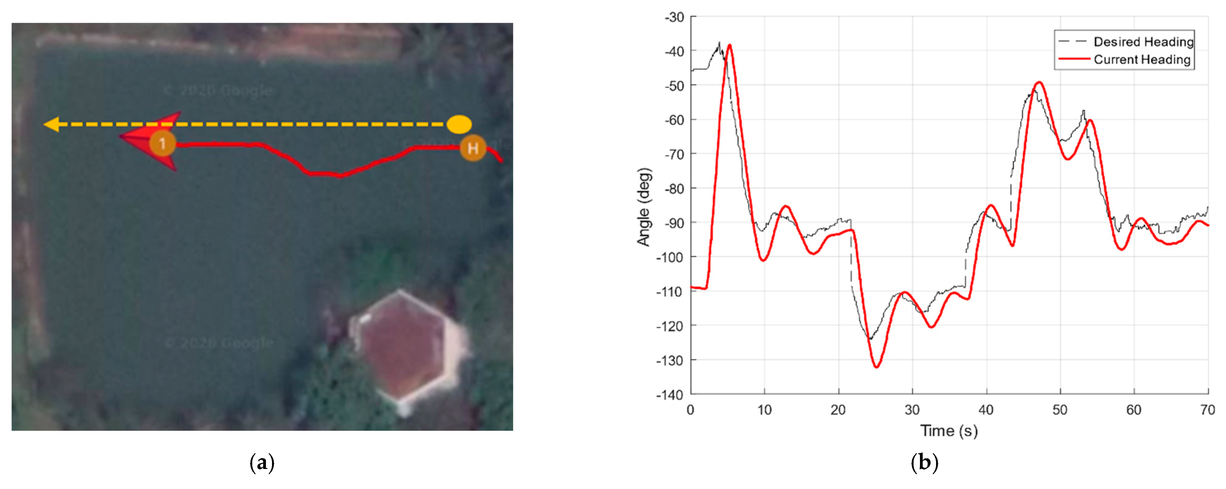
In this experiment, USV2000 is planned to follow a straight line. During operation, the vessel must avoid any dynamic obstacle upon detection, then return along the original global path as fast as possible. The type of obstacle deployed is another moving vessel (Figure 17), which is frequently encountered in practice. All vessels must obey COLOREGS law. Three typical situations are taken into consideration: head-on, overtaking and crossing. While in a head-on case, USV2000 encounters an obstacle moving straight towards; the overtaking situation requires that USV2000 bypass an obstacle moving away from it. In crossing cases, USV2000 is required to avoid an obstacle coming from the right. While USV2000 performs collision avoidance, according to COLOREGS law, the targeted obstacle must maintain its speed and heading. To measure the distance to the obstacle, LiDAR is used. Throughout the experiments, the obstacle’s heading is given in advance. Parameters of the advanced SBG are listed in Table 8.
Experimental results in all three situations (Figure 18, Figure 19 and Figure 20) show that the vessel manages to avoid obstacles and maintain a safe distance during operation. After successful obstacle avoidance, the vessel immediately returns to the original global path, implying that the algorithm does not affect the path following’s performance. It is noticeable that the path’s length in the overtaking case is longer than that of other cases because the relative velocity between vessel and obstacle is smaller. There are abrupt changes in the desired heading’s plot, but USV2000 is flexible enough to perform heading tracking at an acceptable degree, thereby elegantly accomplishing those missions.
7. Conclusions
In this paper, we embed into our newly built USV prototype, namely, VIAM-USV2000, various advanced autonomous capabilities to satisfactorily carry out missions in confined riverine environments in Vietnam and other similar tropical regions. First, a B-Spline path planner is enhanced in that it not only meets the limiting curvature but also exhibits enough flexibility to avoid static obstacles. To smoothly track any arbitrary parameterized curve, we propose a continuous LOS path follower based on a Newton–Raphson iterative procedure that features a continuous projection of the vessel’s center of navigation onto the curve. An advanced SBG law is also proposed to plan a trapezium-like local path for avoiding dynamic obstacles on the fly. Simulated and experimental results show that the proposed B-Spline path planner and continuous LOS path follower enable the vessel to smoothly maneuver with moderate CTE through consecutive, sharp bends. During operation, the safety issue is guaranteed when the vessel always succeeds in avoiding and maintaining a minimum distance from any dynamic obstacle in various circumstances. It is also important to restate that all algorithms are realized by an efficient implementation of hardware–software infrastructure, thereby maintaining modularity, specialty and parallelity to maximize resource usage and facilitate simple maintenance, replacement and upgrade. To our belief, this USV model can open up many real-world applications such as environmental monitoring in a variety of remote areas all around the world.
Author Contributions
Conceptualization, N.-H.T. and H.-S.C.; methodology, N.-H.T.; software, Q.-H.P. and J.-H.L.; validation, N.-H.T. and H.-S.C.; formal analysis, N.-H.T.; investigation, Q.-H.P. and J.-H.L.; resources, N.-H.T. and Q.-H.P.; data curation, N.-H.T. and Q.-H.P.; writing—original draft preparation, N.-H.T. and Q.-H.P. and J.-H.L.; writing—review and editing, N.-H.T. and H.-S.C. and Q.-H.P.; supervision, N.-H.T. and H.-S.C.; project administration, N.-H.T.; funding acquisition, N.-H.T. and H.-S.C. All authors have read and agreed to the published version of the manuscript.
Funding
This research was supported by the Unmanned Vehicles Core Technology Research and Development Program through the National Research Foundation of Korea (NRF) and the Unmanned Vehicle Advanced Research Center (UVARC), funded by the Ministry of Science and ICT, the Republic of Korea (NRF-2020M3C1C1A02086321).
Acknowledgments
We acknowledge the support of time and facilities from Laboratory of Advance Design and Manufacturing Processes (ADMP) and Innovation Fablab, Ho Chi Minh City University of Technology (HCMUT), VNU-HCM for this study.
Conflicts of Interest
The authors declare no conflict of interest.
References
- Curcio, J.; Leonard, J.; Patrikalakis, A. SCOUT—A low cost autonomous surface platform for research in cooperative autonomy. In Proceedings of the OCEANS 2005 MTS/IEEE, Washington, DC, USA, 17–23 September 2006. [Google Scholar]
- Hitz, G.; Gotovos, A.; Pomerleau, F.; Garneau, M.-É.; Pradalier, C.; Krause, A.; Siegwart, R.Y. Fully autonomous focused exploration for robotic environmental monitoring. In Proceedings of the 2014 IEEE International Conference on Robotics and Automation (ICRA), Hong Kong, China, 31 May–7 June 2014. [Google Scholar]
- Yang, T.; Hsiung, S.; Kuo, C.; Tsai, Y.; Peng, K.; Hsieh, Y.; Shen, Z.; Feng, J.; Kuo, C. Development of unmanned surface vehicle for water quality monitoring and measurement. In Proceedings of the 2018 IEEE International Conference on Applied System Invention (ICASI), Chiba, Japan, 13–17 April 2018. [Google Scholar]
- Manley, J.E. Unmanned surface vehicles, 15 years of development. In Proceedings of the OCEANS 2008, Quebec City, QC, Canada, 15–18 September 2008. [Google Scholar]
- Liu, Z.; Zhang, Y.; Yu, X.; Yuan, C. Unmanned surface vehicles: An overview of developments and challenges. Annu. Rev. Control 2016, 41, 71–93. [Google Scholar] [CrossRef]
- Wang, W.; Gheneti, B.; Mateos, L.A.; Duarte, F.; Ratti, C.; Rus, D. Roboat: An Autonomous Surface Vehicle for Urban Waterways. In Proceedings of the 2019 IEEE/RSJ International Conference on Intelligent Robots and Systems (IROS), Macau, China, 3–8 November 2019. [Google Scholar]
- Wang, W.; Shan, T.; Leoni, P.; Fernandez-Gutierrez, D.; Meyers, D.; Ratti, C.; Rus, D. Roboat II: A Novel Autonomous Surface Vessel for Urban Environments. In Proceedings of the 2020 IEEE/RSJ International Conference on Intelligent Robots and Systems (IROS), Las Vegas, NV, USA, 25–29 October 2020. [Google Scholar]
- Tran, N.-H.; Nguyen, T.-C.; Tran, V.-T.; Nguyen, V.-C.; Nguyen, T.-N. The Design of an VIAM-USVI000 Unmanned Surface Vehicle for Environmental Monitoring Applications. In Proceedings of the 2018 4th International Conference on Green Technology and Sustainable Development (GTSD), Ho Chi Minh City, Vietnam, 23–24 November 2018. [Google Scholar]
- Tran, N.-H.; Nguyen, A.-D.; Nguyen, T.-N. A Genetic Algorithm Application in Planning Path Using B-Spline Model for Autonomous Underwater Vehicle (AUV). Appl. Mech. Mater. 2020, 902, 54–64. [Google Scholar] [CrossRef]
- De Boor, C. On calculating with B-splines. J. Approx. Theory 1972, 6, 50–62. [Google Scholar] [CrossRef] [Green Version]
- Katoch, S.; Chauhan, S.S.; Kumar, V. A review on genetic algorithm: Past, present, and future. Multimed. Tools Appl. 2021, 80, 8091–8126. [Google Scholar] [CrossRef] [PubMed]
- LaValle, S.M.; James, J.; Kuffner, J. Randomized Kinodynamic Planning. Int. J. Robot. Res. 2001, 20, 378–400. [Google Scholar] [CrossRef]
- Dubins, L. On Curves of Minimal Length with a Constraint on Average Curvature, and with Prescribed Initial and Terminal Positions and Tangents. Am. J. Math. 1957, 79, 497–516. [Google Scholar] [CrossRef]
- Fossen, T.I. Handbook of Marine Craft Hydrodynamics and Motion Control; John Wiley & Sons: Hoboken, NJ, USA, 2011; pp. 254–266. [Google Scholar]
- Fox, D.; Burgard, W.; Thrun, S. The dynamic window approach to collision avoidance. IEEE Robot. Autom. Mag. 1997, 4, 23–33. [Google Scholar] [CrossRef] [Green Version]
- Borenstein, J.; Koren, Y. The vector field histogram-fast obstacle avoidance for mobile robots. IEEE Trans. Robot. Autom. 1991, 7, 278–288. [Google Scholar] [CrossRef] [Green Version]
- Fiorini, P.; Shiller, Z. Motion Planning in Dynamic Environments Using Velocity Obstacles. Int. J. Robot. Res. 1998, 17, 760–772. [Google Scholar] [CrossRef]
- Kuwata, Y.; Wolf, M.T.; Zarzhitsky, D.; Huntsberger, T.L. Safe Maritime Autonomous Navigation with COLREGS, Using Velocity Obstacles. IEEE J. Ocean. Eng. 2014, 39, 110–119. [Google Scholar] [CrossRef]
- Moe, S.; Pettersen, K.Y. Set-based Line-of-Sight (LOS) path following with collision avoidance for underactuated unmanned surface vessel. In Proceedings of the 2016 24th Mediterranean Conference on Control and Automation (MED), Athens, Greece, 21–24 June 2016. [Google Scholar]
- Tran, N.-H.; Vu, M.-H.; Nguyen, T.-C.; Phan, M.-T.; Pham, Q.-H. Implementation and Enhancement of Set-Based Guidance by Velocity Obstacle along with LiDAR for Unmanned Surface Vehicles. In Proceedings of the 2020 5th International Conference on Green Technology and Sustainable Development (GTSD), Ho Chi Minh City, Vietnam, 27–28 November 2020. [Google Scholar]
- Hoschek, J.; Lasser, D. Fundamentals of Computer Aided Geometric Design; AK Peters, Ltd.: Natick, MA, USA, 1996. [Google Scholar]
- Tiller, W.; Piegl, L. The NURBS Book; Springer: Berlin, Germany, 1997. [Google Scholar]
- Bäck, T. Evolutionary Algorithms in Theory and Practice: Evolution Strategies, Evolutionary Programming, Genetic Algorithms; Oxford University Press: New York, NY, USA, 1996. [Google Scholar]
- Farin, G.; Hoschek, J.; Kim, M.-S. A History of Curves and Surfaces in CAGD. In Handbook of Computer Aided Geometric Design; Elsevier: Amsterdam, The Netherlands, 2002; pp. 1–21. [Google Scholar]
Figure 1.
Catamaran design of USV2000 in (a); USV2000 during operation in (b).

Figure 2.
Diagram describing connections between different components of USV2000.

Figure 3.
Diagram illustrating connections among different software in VIAM-USV-VC.

Figure 4.
Functionalities of VIAM-USV-GC: itinerary monitoring (a), mission planning (b), parameter tuning (c) and real-time data plotting (d).
Figure 4.
Functionalities of VIAM-USV-GC: itinerary monitoring (a), mission planning (b), parameter tuning (c) and real-time data plotting (d).

Figure 5.
Path planning to avoid static obstacles.

Figure 6.
Continuous LOS path following.

Figure 7.
Dynamic obstacle avoidance by VO: our vessel (purple) needs to avoid another one (red).

Figure 8.
Advanced SBG.

Figure 9.
Simulink model of the overall system with B-Spline path planner and continuous LOS path follower.
Figure 9.
Simulink model of the overall system with B-Spline path planner and continuous LOS path follower.

Figure 10.
Simulated result of path planner: path that meets (blue) and does not (red) meet the limiting curvature are shown in (a); their corresponding curvature plots in (b).
Figure 10.
Simulated result of path planner: path that meets (blue) and does not (red) meet the limiting curvature are shown in (a); their corresponding curvature plots in (b).

Figure 11.
Simulated result of path follower: the traveled path and the corresponding curvature plot in case 1 (a,b) and case 2 (c,d).
Figure 11.
Simulated result of path follower: the traveled path and the corresponding curvature plot in case 1 (a,b) and case 2 (c,d).


Figure 12.
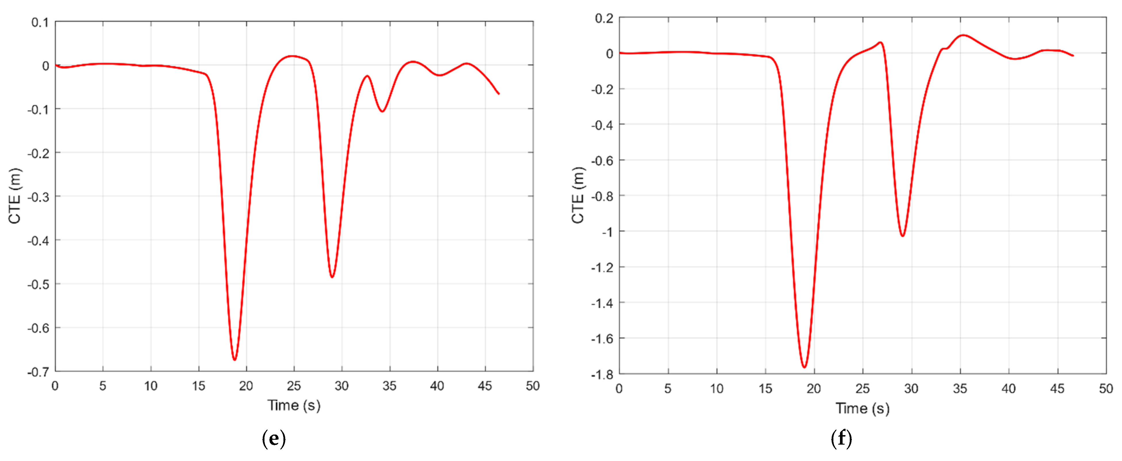
Comparisons of control and guidance performance for two cases in terms of heading error (a,c); control signal (b,d) and CTE (e,f).
Figure 12.
Comparisons of control and guidance performance for two cases in terms of heading error (a,c); control signal (b,d) and CTE (e,f).


Figure 13.
Approximately interpolate B-Spline curve from GPS data in (a); curvature analysis of USV2000 in (b).
Figure 13.
Approximately interpolate B-Spline curve from GPS data in (a); curvature analysis of USV2000 in (b).

Figure 14.
Planned B-Spline path by path planner in GCS in (a); traveled path in (b).

Figure 15.
Curvature analysis of the planned and traveled paths.

Figure 16.
Results of heading error (a), PWM signal (b) and CTE (c) throughout the mission.

Figure 17.
Targeted vessel being an obstacle in (a); obstacle avoidance process in (b).

Figure 18.
Dynamic obstacle avoidance in case of head-on: USV2000′s path (red) and obstacle’s path (yellow) are shown in (a); heading-tracking analysis in (b); obstacle avoidance process with evolving pair of avoiding directions (black) in (c–e).
Figure 18.
Dynamic obstacle avoidance in case of head-on: USV2000′s path (red) and obstacle’s path (yellow) are shown in (a); heading-tracking analysis in (b); obstacle avoidance process with evolving pair of avoiding directions (black) in (c–e).

Figure 19.
Dynamic obstacle avoidance in case of overtaking: USV2000′s path (red) and obstacle’s path (yellow) are shown in (a); heading-tracking analysis in (b); obstacle avoidance process with evolving pair of avoiding directions (black) in (c–e).
Figure 19.
Dynamic obstacle avoidance in case of overtaking: USV2000′s path (red) and obstacle’s path (yellow) are shown in (a); heading-tracking analysis in (b); obstacle avoidance process with evolving pair of avoiding directions (black) in (c–e).


Figure 20.
Dynamic obstacle avoidance in case of crossing: USV2000′s path (red) and obstacle’s path (yellow) are shown in (a); heading-tracking analysis in (b); obstacle avoidance process with evolving pair of avoiding directions (black) in (c–e).
Figure 20.
Dynamic obstacle avoidance in case of crossing: USV2000′s path (red) and obstacle’s path (yellow) are shown in (a); heading-tracking analysis in (b); obstacle avoidance process with evolving pair of avoiding directions (black) in (c–e).


Table 1.
Hardware specifications of USV2000.
| Component | Specification |
|---|---|
| Embedded computer | 1× nVIDIA Jetson Nano |
| Microcontroller | 1× STM32F407 |
| Rear thruster | 2× Endura C2 30 |
| Side thruster | 2× BlueRobotics T200 |
| RC controller | 1× RadioLink AT9S |
| LiDAR | 1× Hokuyo UTM-30LX |
| AHRS | 1× Patech RTxQ |
| GNSS receiver | 1× Here+ RTK GNSS |
| Wireless router | 1× TP-Link TL-WR940N |
Table 2.
Algorithm to find the projection of the vessel’s center of navigation onto the curve.
| Input Vessel’s current center of navigation . Parameterized curve . |
| Output Projection onto the curve. |
Process
|
Table 3.
How to choose direction of collision avoidance according to COLOREGS law.
| Case | ||
|---|---|---|
| Overtaking | ||
| Crossing (from left) | ||
| Head-on | ||
| Head-on | ||
| Crossing (from right) | ||
| Overtaking |
Table 4.
Quantitative evalution in control and guidance performance for two cases.
| Criteria | Case 1 | Case 2 |
|---|---|---|
| Length of planned path (m) | 113.8323 | 112.7625 |
| Travelled distance (m) | 111.3862 | 111.7344 |
| Root-mean-square CTE (m) | 0.1754 | 0.4500 |
| Root-mean-square heading error (deg) | 6.0976 | 13.4719 |
| Distance deviation from WP2 (m) | 0.0085 | 0.1498 |
| Distance deviation from WP3 (m) | 0.0040 | 0.0158 |
| Distance deviation from WP4 (m) | 0.0017 | 0.0003 |
| Distance deviation from WP5 (m) | 0.0001 | 0.0001 |
Table 5.
Radius of turning of USV2000.
| Direction | Radius of Turning (m) |
|---|---|
| Counterclockwise | 3.92–4.30 |
| Clockwise | 3.82–4.25 |
Table 6.
Paramters of B-Spline path planner with GA optimization.
| Parameter | Value |
|---|---|
| Degree of B-Spline | 4 |
| Number of generations | 200 |
| Number of individuals per population | 100 |
| Number of selected individuals | 50 |
| Mutation rate | 10% |
Table 7.
Quantitative evalution in control and guidance performance of USV2000.
| Criteria | Value |
|---|---|
| Average speed (m/s) | 0.55 |
| Travelled distance (m) | 118.5311 |
| Root-mean-square CTE (m) | 0.2868 |
| Root-mean-square heading error (deg) | 5.7701 |
| Distance deviation from WP2 (m) | 0.4762 |
| Distance deviation from WP3 (m) | 0.4509 |
| Distance deviation from WP4 (m) | 0.4306 |
| Distance deviation from WP5 (m) | 0.4466 |
Table 8.
Parameters of the advanced SBG.
| Parameter | Value |
|---|---|
| Safety distance (m) | 2.5 |
| Distance to avoid (m) | 5 |
| Velocity of vessel (m/s) | 1 |
| Velocity of obstacle (m/s) | 0.7 |
| Maximum measurable distance (m) | 30 |
| Minimum measurable distance (m) | 0.1 |
Publisher’s Note: MDPI stays neutral with regard to jurisdictional claims in published maps and institutional affiliations. |
© 2021 by the authors. Licensee MDPI, Basel, Switzerland. This article is an open access article distributed under the terms and conditions of the Creative Commons Attribution (CC BY) license (https://creativecommons.org/licenses/by/4.0/).
Share and Cite
MDPI and ACS Style
Tran, N.-H.; Pham, Q.-H.; Lee, J.-H.; Choi, H.-S. VIAM-USV2000: An Unmanned Surface Vessel with Novel Autonomous Capabilities in Confined Riverine Environments. Machines 2021, 9, 133. https://0-doi-org.brum.beds.ac.uk/10.3390/machines9070133
AMA Style
Tran N-H, Pham Q-H, Lee J-H, Choi H-S. VIAM-USV2000: An Unmanned Surface Vessel with Novel Autonomous Capabilities in Confined Riverine Environments. Machines. 2021; 9(7):133. https://0-doi-org.brum.beds.ac.uk/10.3390/machines9070133
Chicago/Turabian StyleTran, Ngoc-Huy, Quang-Ha Pham, Ji-Hyeong Lee, and Hyeung-Sik Choi. 2021. "VIAM-USV2000: An Unmanned Surface Vessel with Novel Autonomous Capabilities in Confined Riverine Environments" Machines 9, no. 7: 133. https://0-doi-org.brum.beds.ac.uk/10.3390/machines9070133
Note that from the first issue of 2016, this journal uses article numbers instead of page numbers. See further details here.