Do Randomized Algorithms Improve the Efficiency of Minimal Learning Machine?


Abstract
:1. Introduction
2. Methods
2.1. MLM in a Nutshell
2.2. OLS Calculation Methods
3. Experiments and Results
3.1. Details on the Methods
3.2. Datasets
3.3. Experimental Setup
- 1.
- Input layer of size M,
- 2.
- Feedforward layer with sigmoid activation function of size ,
- 3.
- Feedforward layer with sigmoid activation function of size ,
- 4.
- Feedforward layer with sigmoid activation function of size ,
- 5.
- Feedforward layer with sigmoid activation function of size 1,
- 1.
- Input layer of size M,
- 2.
- Feedforward layer with sigmoid activation function of size ,
- 3.
- Feedforward layer with sigmoid activation function of size 1,
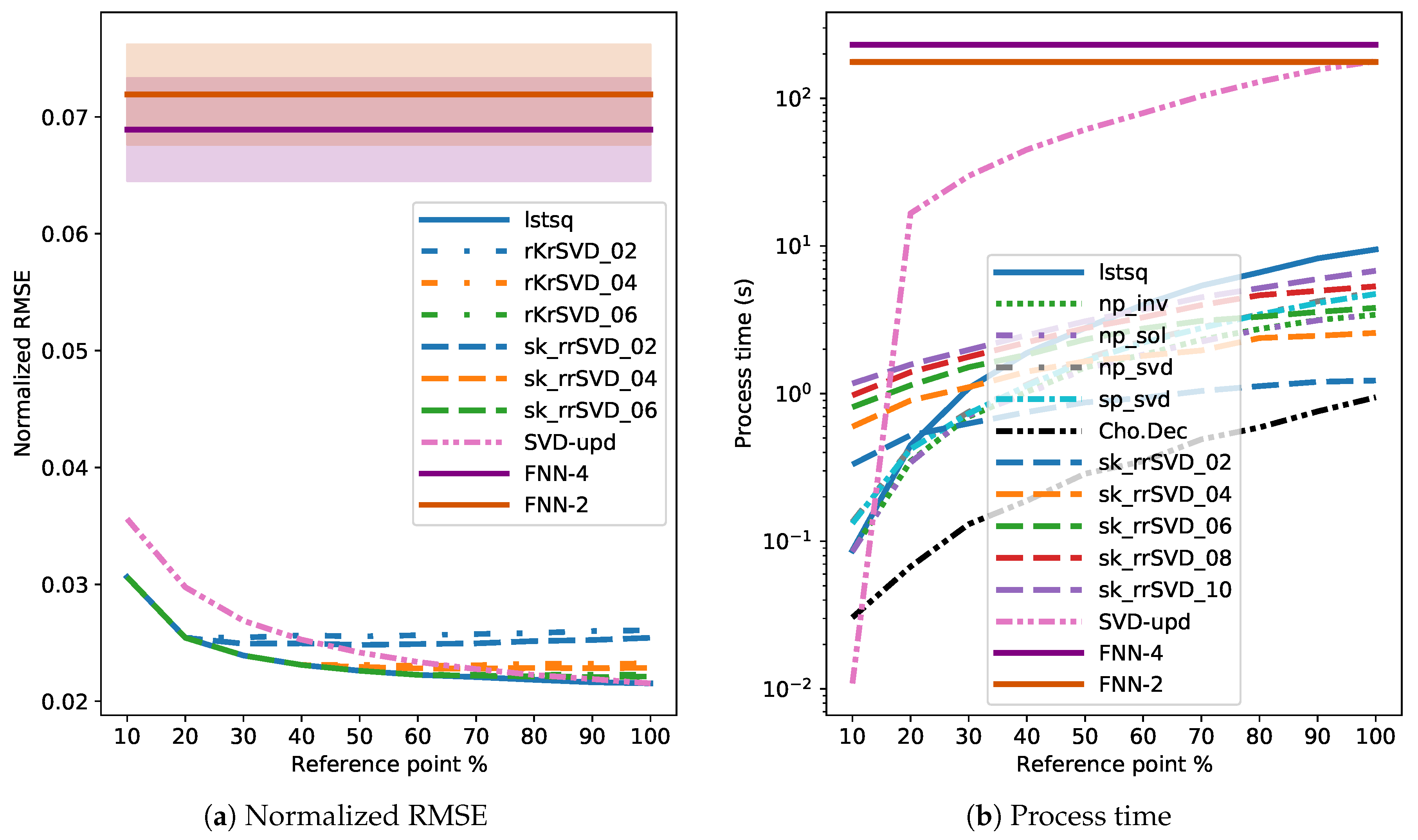
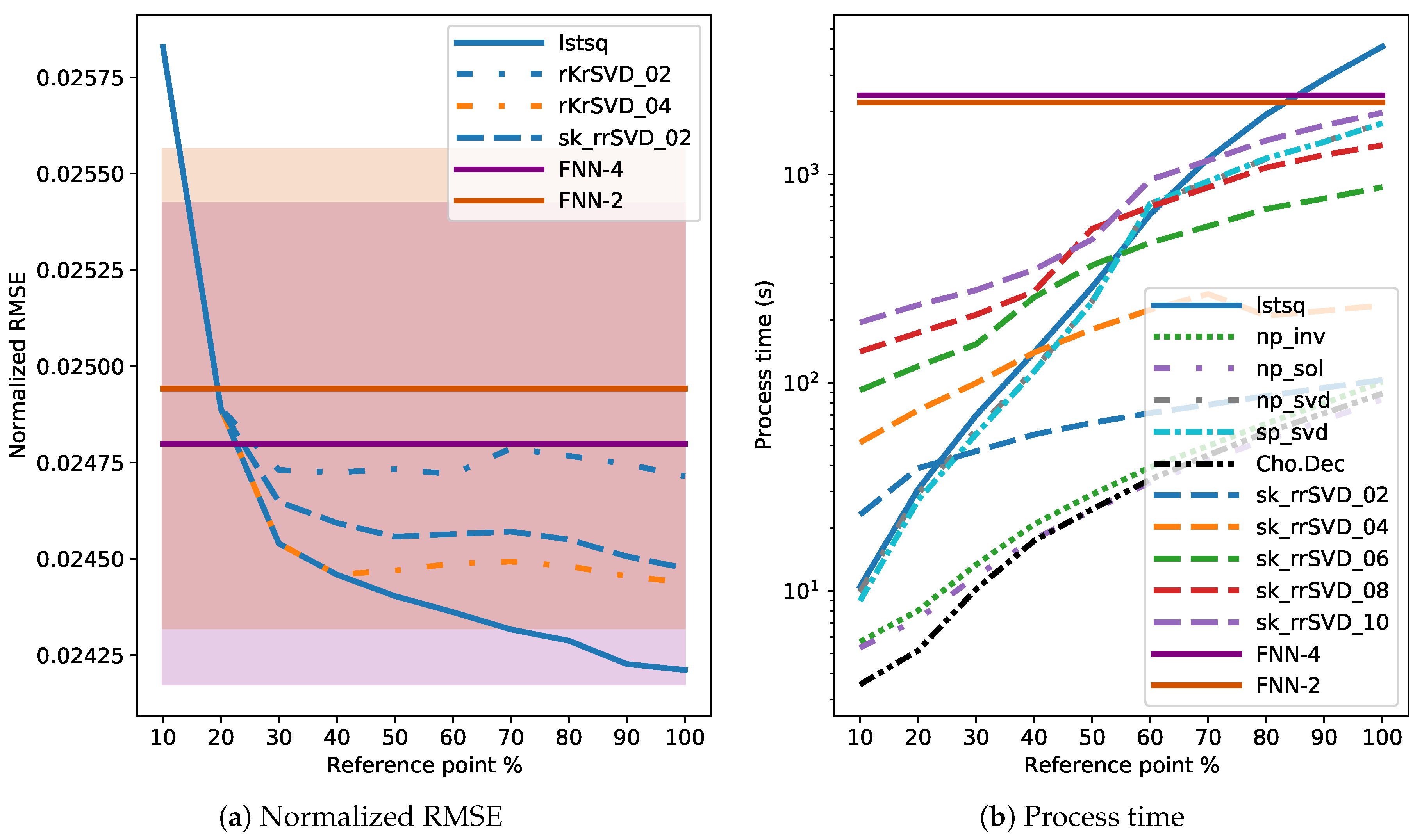
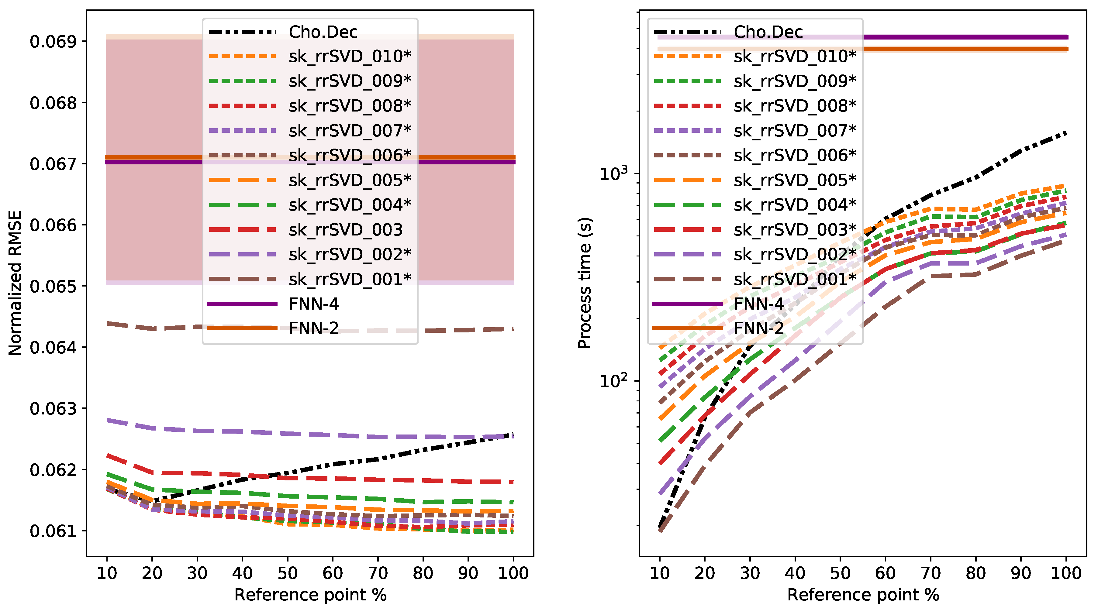
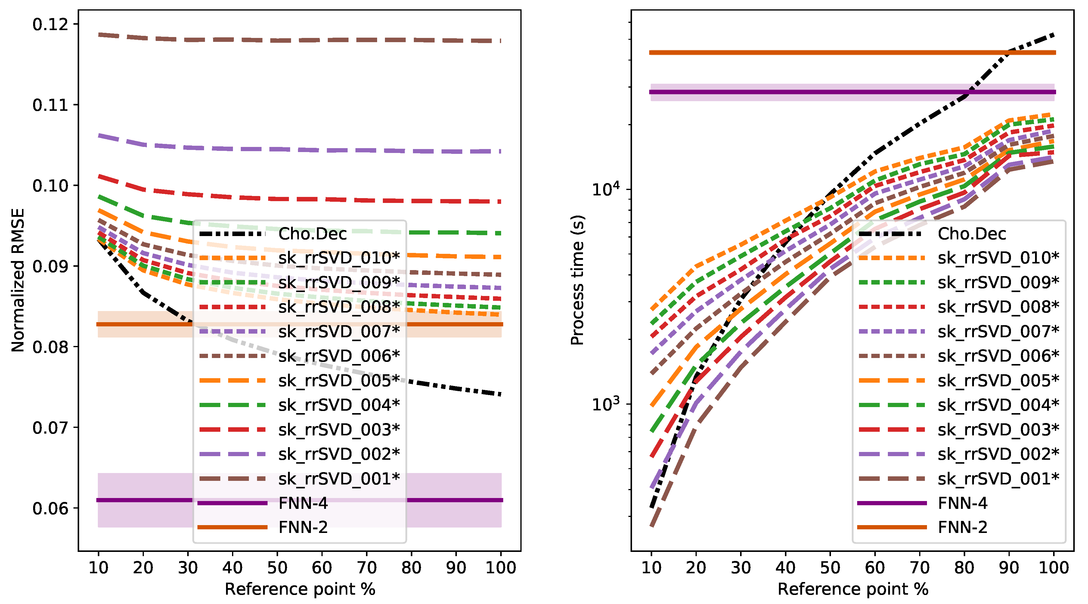
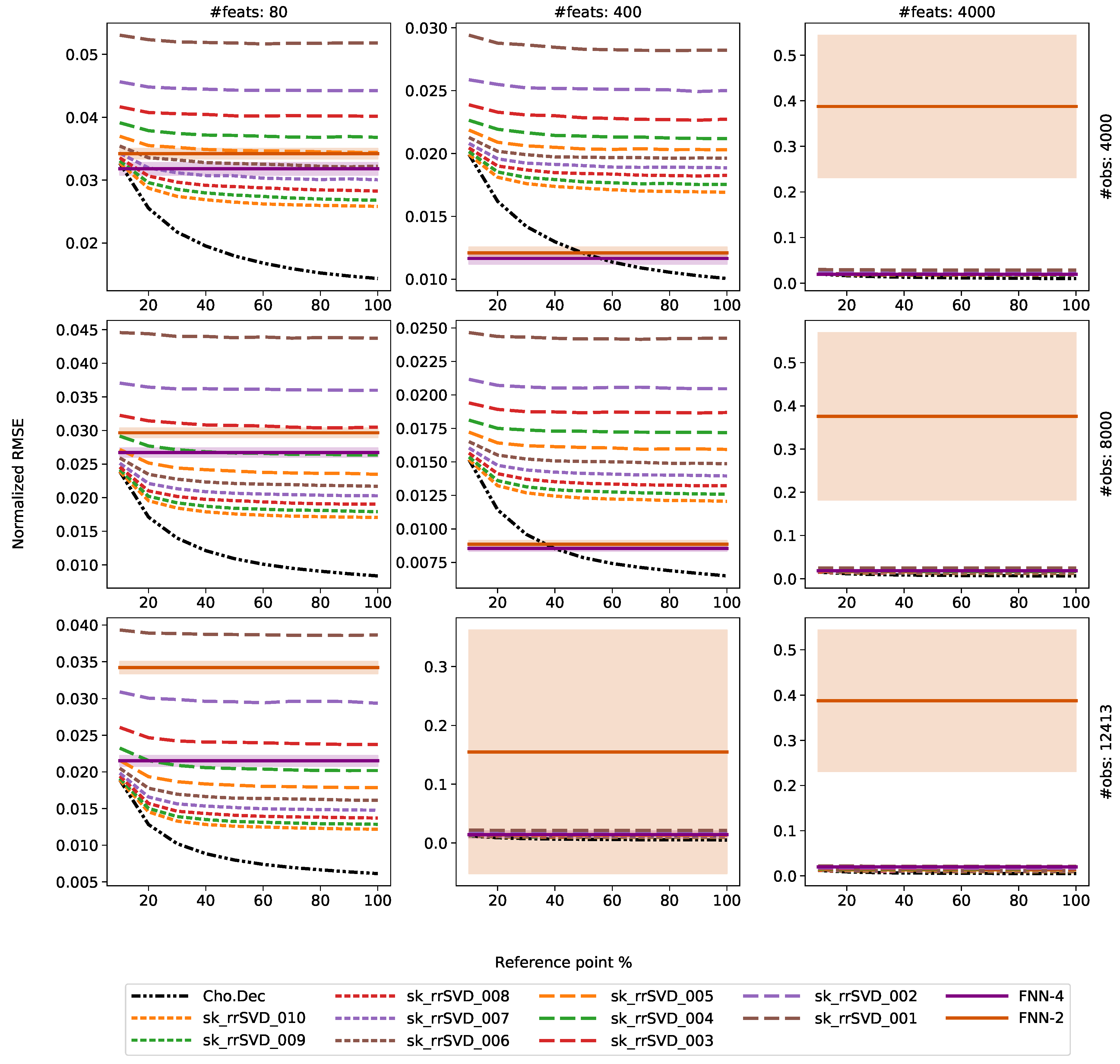
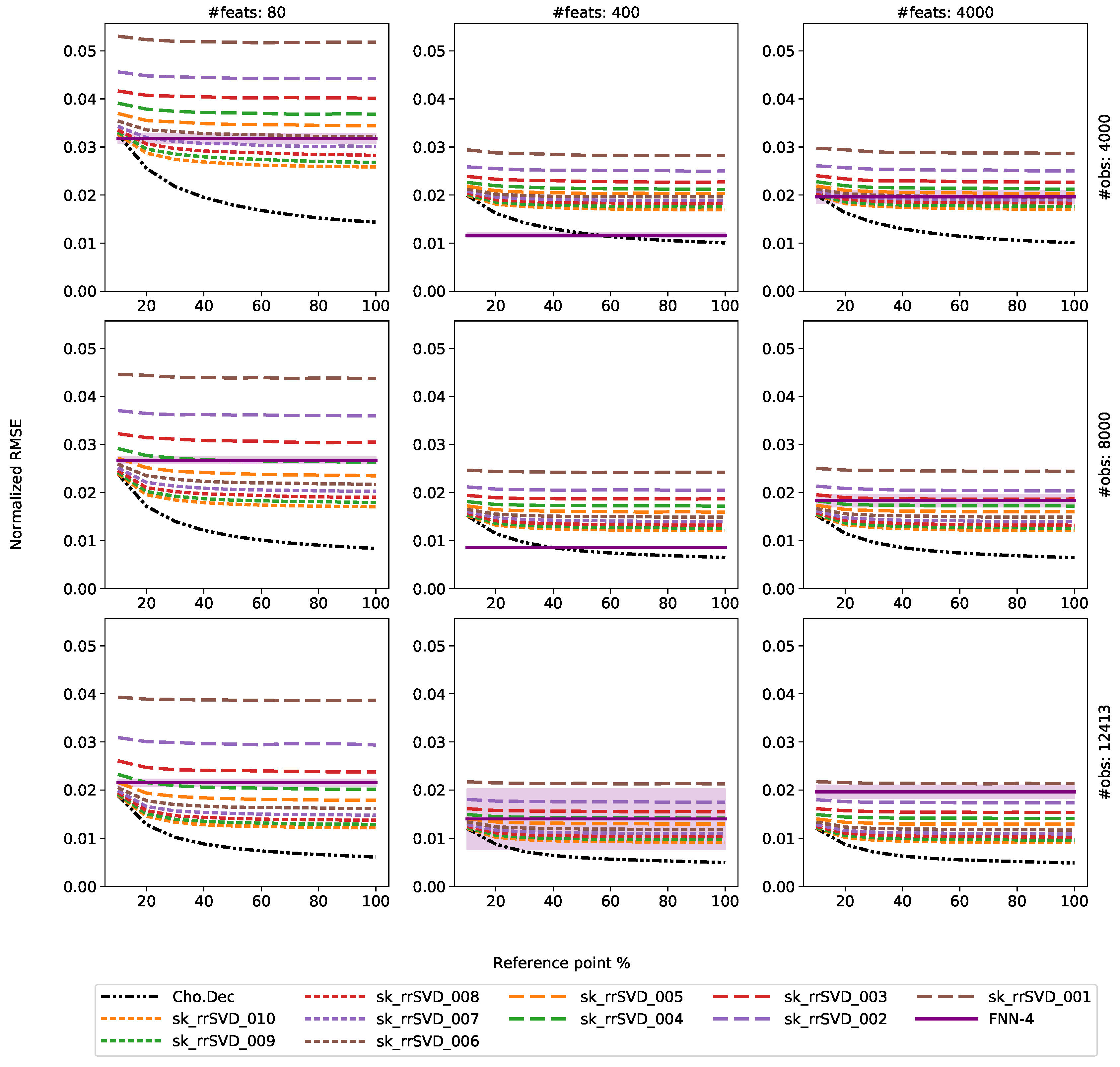
3.4. Results
4. Discussion
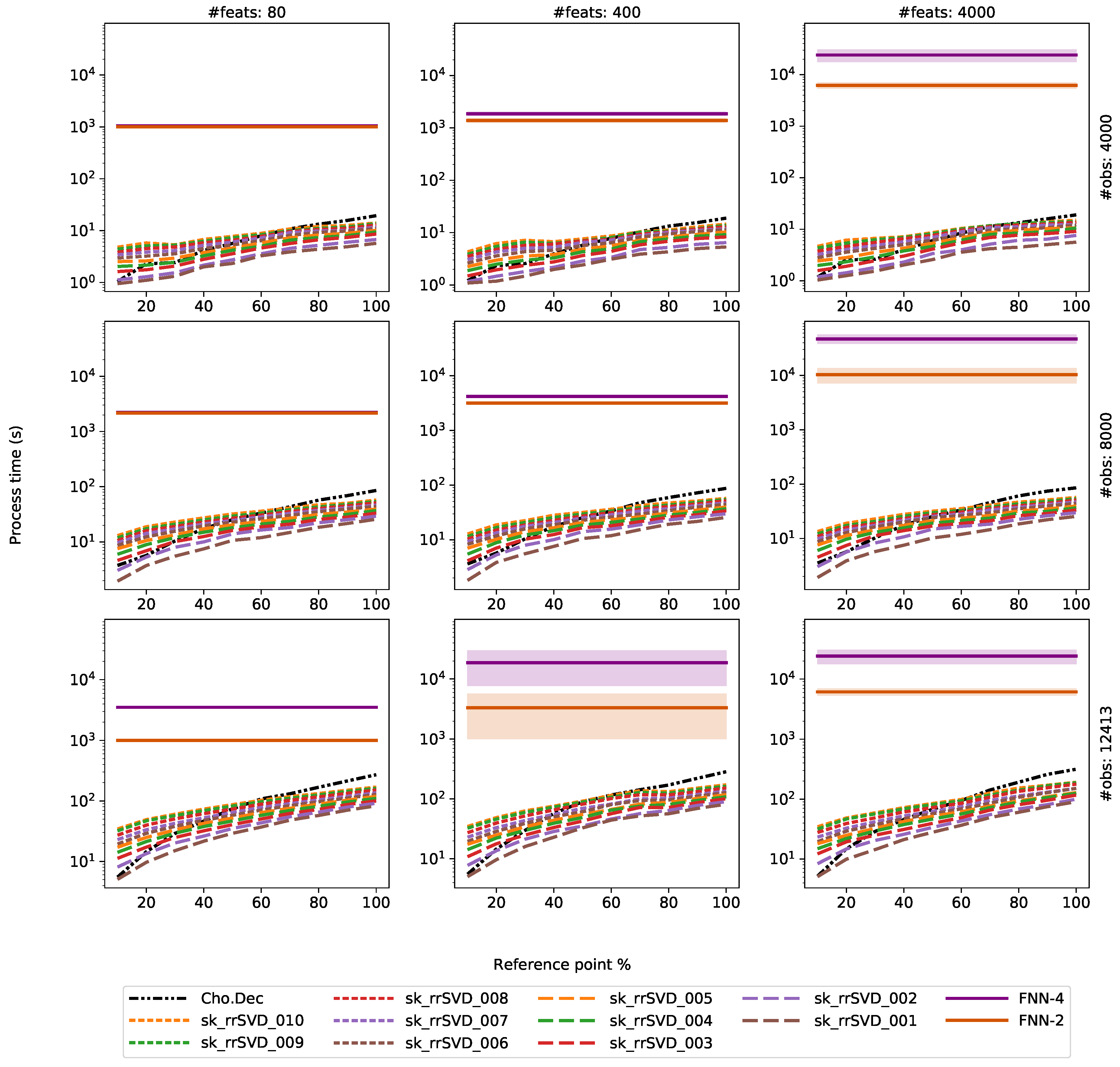
4.1. Comparison of Direct and Randomized Solvers for MLM
4.2. Comparison of MLM to Shallow and Deep FNNs
5. Conclusions and Future Work
- 1.
- If accuracy is the only objective in a prepared situation, one should choose to use a direct solver with the MLM.
- 2.
- If not, randomized solvers provide comparable performance to direct solvers while providing a speedup.
- 3.
- Utilization of linear training technique with a distance-based kernel is computational more efficient than nonlinear optimizers needed for the FNN models. In general, the MLM outperformed the shallow and deep FNNs with fixed architecture, with one exception. Especially, in cases of thousands of features, as with the experiments for the Au dataset here, the MLM is the recommended technique from both training time and model accuracy perspectives.
Supplementary Materials
Author Contributions
Funding
Acknowledgments
Conflicts of Interest
Appendix A. MLM vs. FNN


Appendix B. Au38Q


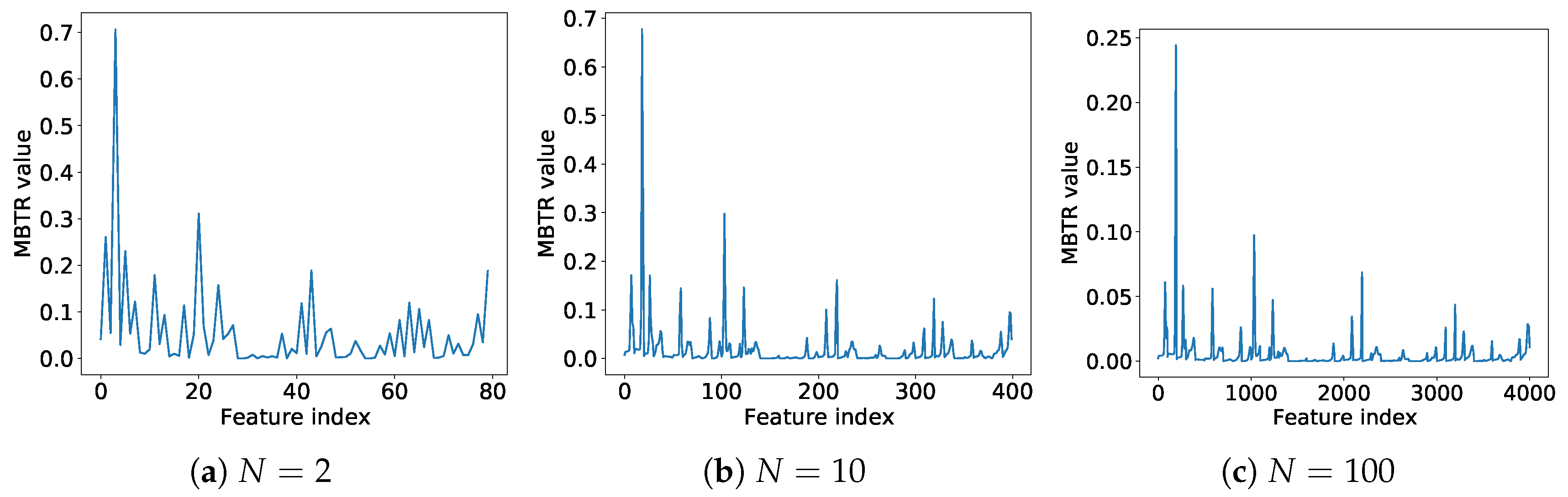
Appendix C. Au38Q MBTR-K3 Dataset and Its Variants

References
- De Souza Junior, A.H.; Corona, F.; Miche, Y.; Lendasse, A.; Barreto, G.A.; Simula, O. Minimal Learning Machine: A New Distance-Based Method for supervised Learning. In International Work-Conference on Artificial Neural Networks; Springer: Berlin/Heidelberg, Germany, 2013; pp. 408–416. [Google Scholar]
- De Souza Junior, A.H.; Corona, F.; Barreto, G.A.; Miche, Y.; Lendasse, A. Minimal Learning Machine: A novel supervised distance-based approach for regression and classification. Neurocomputing 2015, 164, 34–44. [Google Scholar] [CrossRef]
- Pihlajamäki, A.; Hämäläinen, J.; Linja, J.; Nieminen, P.; Malola, S.; Kärkkäinen, T.; Häkkinen, H. Monte Carlo Simulations of Au38(SCH3)24 Nanocluster Using Distance-Based Machine Learning Methods. J. Phys. Chem. 2020, 124, 23. [Google Scholar] [CrossRef]
- Marinho, L.B.; Almeida, J.S.; Souza, J.W.M.; Albuquerque, V.H.C.; Rebouças Filho, P.P. A novel mobile robot localization approach based on topological maps using classification with reject option in omnidirectional images. Expert Syst. Appl. 2017, 72, 1–17. [Google Scholar] [CrossRef]
- Coelho, D.N.; Barreto, G.A.; Medeiros, C.M.S.; Santos, J.D.A. Performance comparison of classifiers in the detection of short circuit incipient fault in a three-phase induction motor. In Proceedings of the 2014 IEEE Symposium on Computational Intelligence for Engineering Solutions (CIES), Orlando, FL, USA, 9–12 December 2014; pp. 42–48. [Google Scholar]
- Pekalska, E.; Duin, R.P. Automatic pattern recognition by similarity representations. Electron. Lett. 2001, 37, 159–160. [Google Scholar] [CrossRef]
- Pekalska, E.; Paclik, P.; Duin, R.P. A generalized kernel approach to dissimilarity-based classification. J. Mach. Learn. Res. 2001, 2, 175–211. [Google Scholar]
- Balcan, M.F.; Blum, A.; Srebro, N. A theory of learning with similarity functions. Mach. Learn. 2008, 72, 89–112. [Google Scholar] [CrossRef]
- Zerzucha, P.; Daszykowski, M.; Walczak, B. Dissimilarity partial least squares applied to non-linear modeling problems. Chemom. Intell. Lab. Syst. 2012, 110, 156–162. [Google Scholar] [CrossRef]
- Sanchez, J.D.; Rêgo, L.C.; Ospina, R. Prediction by Empirical Similarity via Categorical Regressors. Mach. Learn. Knowl. Extr. 2019, 1, 38. [Google Scholar] [CrossRef] [Green Version]
- Kärkkäinen, T. Extreme minimal learning machine: Ridge regression with distance-based basis. Neurocomputing 2019, 342, 33–48. [Google Scholar] [CrossRef]
- Hämäläinen, J.; Alencar, A.S.; Kärkkäinen, T.; Mattos, C.L.; Júnior, A.H.S.; Gomes, J.P. Minimal Learning Machine: Theoretical Results and Clustering-Based Reference Point Selection. arXiv 2019, arXiv:1909.09978v2. To appear. [Google Scholar]
- Florêncio, J.A.; Oliveira, S.A.; Gomes, J.P.; Neto, A.R.R. A new perspective for Minimal Learning Machines: A lightweight approach. Neurocomputing 2020, 401, 308–319. [Google Scholar] [CrossRef]
- Hämäläinen, J.; Kärkkäinen, T. Newton’s Method for Minimal Learning Machine. In Computational Sciences and Artificial Intelligence in Industry—New Digital Technologies for Solving Future Societal and Economical Challenges; Springer Nature: Cham, Switzerland, 2020. [Google Scholar]
- LeCun, Y.; Bengio, Y.; Hinton, G. Deep learning. Nature 2015, 521, 436–444. [Google Scholar] [CrossRef] [PubMed]
- Dias, M.L.D.; de Souza, L.S.; da Rocha Neto, A.R.; de Souza Junior, A.H. Opposite neighborhood: A new method to select reference points of minimal learning machines. In Proceedings of the European Symposium on Artificial Neural Networks, Computational Intelligence and Machine Learning—ESANN, Bruges, Belgium, 25–27 April 2018; pp. 201–206. [Google Scholar]
- Florêncio, J.A.V.; Dias, M.L.D.; da Rocha Neto, A.R.; de Souza Júnior, A.H. A Fuzzy C-Means-based Approach for Selecting Reference Points in Minimal Learning Machines; Barreto, G.A., Coelho, R., Eds.; Springer: Cham, Switzerland, 2018; pp. 398–407. [Google Scholar]
- Mesquita, D.P.P.; Gomes, J.P.P.; Souza Junior, A.H. Ensemble of Efficient Minimal Learning Machines for Classification and Regression. Neural Process. Lett. 2017, 46, 751–766. [Google Scholar] [CrossRef]
- Grigorievskiy, A.; Miche, Y.; Käpylä, M.; Lendasse, A. Singular value decomposition update and its application to (Inc)-OP-ELM. Neurocomputing 2016, 174, 99–108. [Google Scholar] [CrossRef]
- Martinsson, P.G.; Rokhlin, V.; Tygert, M. A randomized algorithm for the decomposition of matrices. Appl. Comput. Harmon. Anal. 2011, 30, 47–68. [Google Scholar] [CrossRef] [Green Version]
- Shabat, G.; Shmueli, Y.; Aizenbud, Y.; Averbuch, A. Randomized LU decomposition. Appl. Comput. Harmon. Anal. 2018, 44, 246–272. [Google Scholar] [CrossRef] [Green Version]
- Abdelfattah, S.; Haidar, A.; Tomov, S.; Dongarra, J. Analysis and Design Techniques towards High-Performance and Energy-Efficient Dense Linear Solvers on GPUs. IEEE Trans. Parallel Distrib. Syst. 2018, 29, 2700–2712. [Google Scholar] [CrossRef]
- Gonzalez, T.F. Clustering to minimize the maximum intercluster distance. Theor. Comput. Sci. 1985, 38, 293–306. [Google Scholar] [CrossRef] [Green Version]
- Huang, G.B.; Zhu, Q.Y.; Siew, C.K. Extreme learning machine: A new learning scheme of feedforward neural networks. In Proceedings of the 2004 International Joint Conference on Neural Networks (IJCNN), Budapest, Hungary, 25–29 July 2004; pp. 985–990. [Google Scholar]
- Kingma, D.P.; Ba, J. Adam: A method for stochastic optimization. arXiv 2014, arXiv:1412.6980. [Google Scholar]
- Oliphant, T.E. A Guide to NumPy; Trelgol Publishing: USA, 2006. [Google Scholar]
- Virtanen, P.; Gommers, R.; Oliphant, T.E.; Haberland, M.; Reddy, T.; Cournapeau, D.; Burovski, E.; Peterson, P.; Weckesser, W.; Bright, J.; et al. SciPy 1.0–Fundamental Algorithms for Scientific Computing in Python. arXiv 2019, arXiv:1907.10121. [Google Scholar] [CrossRef] [Green Version]
- Pedregosa, F.; Varoquaux, G.; Gramfort, A.; Michel, V.; Thirion, B.; Grisel, O.; Blondel, M.; Prettenhofer, P.; Weiss, R.; Dubourg, V.; et al. Scikit-learn: Machine Learning in Python. J. Mach. Learn. Res. 2011, 12, 2825–2830. [Google Scholar]
- Stewart, G.W. On the Early History of the Singular Value Decomposition. SIAM Rev. 1993, 35, 551–566. [Google Scholar] [CrossRef] [Green Version]
- Tikhonov, A.N.; Arsenin, V.J. Solution of Ill-Posed Problems; Winston&Sons: New York, NY, USA, 1977. [Google Scholar]
- Halko, N.; Martinsson, P.G.; Tropp, J.A. Finding Structure with Randomness: Stochastic Algorithms for Constructing Approximate matrix Decompositions. ACM Tech. Rep. 2009. [Google Scholar] [CrossRef]
- Kruskal, W.H.; Wallis, W.A. Use of ranks in one-criterion variance analysis. J. Am. Stat. Assoc. 1952, 47, 583–621. [Google Scholar] [CrossRef]
- Juarez-Mosqueda, R.; Sami, M.; Hannu, H. Ab initio molecular dynamics studies of Au38(SR)24 isomers under heating. Eur. Phys. J. 2019, 73. [Google Scholar] [CrossRef]
- Dua, D.; Graff, C. UCI Machine Learning Repository. California, USA 2017. Available online: http://archive.ics.uci.edu/ml (accessed on 13 November 2020).
- Torgo, L. Airplane Companies Stocks; Faculdade de Ciências da Universidade do Porto: Porto, Portugal, 1991. [Google Scholar]
- University of Toronto. Delve Datasets; University of Toronto: Toronto, ON, Cananda, 1996. [Google Scholar]
- LeCun, Y.; Bottou, L.; Bengio, Y.; Haffner, P. Gradient-based learning applied to document recognition. Proc. IEEE 1998, 86, 2278–2323. [Google Scholar] [CrossRef] [Green Version]
- Khamparia, A.; Singh, K.M. A systematic review on deep learning architectures and applications. Expert Syst. 2019, 36, e12400. [Google Scholar] [CrossRef]
- Abadi, M.; Agarwal, A.; Barham, P.; Brevdo, E.; Chen, Z.; Citro, C.; Corrado, G.S.; Davis, A.; Dean, J.; Devin, M.; et al. TensorFlow: Large-Scale Machine Learning on Heterogeneous Systems. arXiv 2015, arXiv:1603.04467. [Google Scholar]
- Emmert-Streib, F.; Dehmer, M. Understanding Statistical Hypothesis Testing: The Logic of Statistical Inference. Mach. Learn. Knowl. Extr. 2019, 1, 54. [Google Scholar] [CrossRef] [Green Version]
- Zhou, Z.H.; Feng, J. Deep forest. Natl. Sci. Rev. 2018, 6, 74–86. [Google Scholar] [CrossRef]
- Li, H.B.; Huang, T.Z.; Zhang, Y.; Liu, X.P.; Gu, T.X. Chebyshev-type methods and preconditioning techniques. Appl. Math. Comput. 2011, 218, 260–270. [Google Scholar] [CrossRef]
- Hadjidimos, A. Accelerated overrelaxation method. Math. Comput. 1978, 32, 149–157. [Google Scholar] [CrossRef]
- Qian, H.; Eckenhoff, W.T.; Zhu, Y.; Pintauer, T.; Jin, R. Total Structure Determination of Thiolate-Protected Au38 Nanoparticles. J. Am. Chem. Soc. 2010, 132, 8280–8281. [Google Scholar] [CrossRef] [PubMed]
- Huo, H.; Rupp, M. Unified Representation of Molecules and Crystals for Machine Learning. arXiv 2017, arXiv:1704.06439. [Google Scholar]
- Himanen, L.; Jäger, M.O.J.; Morooka, E.V.; Federici Canova, F.; Ranawat, Y.S.; Gao, D.Z.; Rinke, P.; Foster, A.S. DScribe: Library of descriptors for machine learning in materials science. Comput. Phys. Commun. 2020, 247, 106949. [Google Scholar] [CrossRef]


| Name | Abbreviation | Source |
|---|---|---|
| np.lstsq | Lstsq_X | [26] |
| np.inverse | np_inv_X | [26] |
| np.solve | np_sol_X | [26] |
| Cholesky decomposition | Cho.Dec | [26,27] |
| np.svd | np_svd | [26] |
| sp.svd | sp_svd | [27] |
| rank K random SVD | rKrSVD_XX | [20] |
| sk rank random SVD | sk_rrSVD_XX | [28] |
| SVD update | SVD–upd | [19] |
| Dataset name | Acronym | # Obser. | # Feat. | # Uniq. Targets | Source |
|---|---|---|---|---|---|
| Breast Cancer Progn. (Wisc.) | BC | 194 | 32 | 94 | [34] |
| Boston Housing | BH | 506 | 13 | 229 | [34] |
| Airplane Companies Stocks | AC | 950 | 9 | 203 | [35] |
| Computer Activity (CPU) | CA | 8192 | 21 | 56 | [36] |
| Census (House 8L) | CE | 22,784 | 8 | 2045 | [36] |
| Mnist | MN | 70,000 | 784 | 10 | [37] |
| Au | AuNx-yk | 12,413 | 4000 | 12,413 | [33] |
| Dataset | BC | BH | AC | CA | CE | |||||
|---|---|---|---|---|---|---|---|---|---|---|
| Method/coef. | 1 × | 1 × | 1 × | 1 × | 1 × | 1 × | 1 × | 1 × | 1 × | 1 × |
| Lstsq | 2.77 | 2.34 | 6.79 | 1.35 | 2.21 | 1.47 | 2.43 | 8.36 | 6.28 | 2.17 |
| Lstsq (nr) | 2.77 | 2.34 | 6.79 | 1.35 | 2.21 | 1.47 | 2.43 | 8.36 | - | - |
| np.inv | 2.77 | 2.34 | 6.79 | 1.35 | 2.21 | 1.47 | 2.43 | 8.36 | 6.28 | 2.17 |
| np.inv (nr) | 2.77 | 2.34 | 6.79 | 1.35 | 2.21 | 1.47 | 2.43 | 8.36 | - | - |
| np.solve | 2.77 | 2.34 | 6.79 | 1.35 | 2.21 | 1.47 | 2.43 | 8.36 | 6.28 | 2.17 |
| np.solve (nr) | 2.77 | 2.34 | 6.79 | 1.35 | 2.21 | 1.47 | 2.43 | 8.36 | - | - |
| np.svd | 2.77 | 2.34 | 6.79 | 1.35 | 2.21 | 1.47 | 2.43 | 8.36 | 6.28 | 2.17 |
| sp.svd | 2.77 | 2.34 | 6.79 | 1.35 | 2.21 | 1.47 | 2.43 | 8.36 | - | - |
| Cho.Dec | 2.77 | 2.34 | 6.79 | 1.35 | 2.21 | 1.47 | 2.43 | 8.36 | 6.28 | 2.17 |
| rKrSVD02 | 2.67 | 2.33 | 7.93 | 1.38 | 2.57 | 1.47 | 2.48 | 8.17 | 6.21 | 2.12 |
| rKrSVD04 | 2.72 | 2.27 | 7.1 | 1.36 | 2.31 | 1.48 | 2.45 | 8.27 | 6.24 | 2.18 |
| rKrSVD06 | 2.75 | 2.37 | 6.86 | 1.36 | 2.23 | 1.46 | 2.44 | 8.39 | 6.27 | 2.18 |
| rKrSVD08 | 2.77 | 2.34 | 6.79 | 1.35 | 2.21 | 1.47 | 2.43 | 8.36 | - | - |
| rKrSVD10 | 2.77 | 2.34 | 6.79 | 1.35 | 2.21 | 1.47 | 2.43 | 8.36 | - | - |
| skrSVD02 | 2.65 | 2.32 | 7.8 | 1.47 | 2.49 | 1.63 | 2.46 | 8.38 | 6.18 | 2.2 |
| skrSVD04 | 2.72 | 2.35 | 6.98 | 1.38 | 2.28 | 1.46 | 2.44 | 8.3 | 6.24 | 2.2 |
| skrSVD06 | 2.75 | 2.37 | 6.84 | 1.36 | 2.22 | 1.45 | 2.43 | 8.39 | 6.27 | 2.17 |
| skrSVD08 | 2.77 | 2.34 | 6.79 | 1.35 | 2.21 | 1.47 | 2.43 | 8.36 | - | - |
| skrSVD10 | 2.77 | 2.34 | 6.79 | 1.35 | 2.21 | 1.47 | 2.43 | 8.36 | - | - |
| SVDU | 2.74 | 2.36 | 7.07 | 1.47 | 2.27 | 1.62 | - | - | - | - |
| MLM (Cholesky Decomposition) | Accuracy | Training Time |
|---|---|---|
| Dataset | rnd. Solver | rnd. Solver |
| BreastCancer | + | − |
| BostonHousing | − | − |
| AirplaneCompanies | − | − |
| ComputerActivity | − | − |
| Census | + | + |
| Mnist | − | + |
| AuN2-4k | − | + |
| AuN2-8k | − | + |
| AuN2-12k | − | + |
| AuN10-4k | − | + |
| AuN10-8k | − | + |
| AuN10-12k | − | + |
| AuN100-4k | − | + |
| AuN100-8k | − | + |
| AuN100-12k | − | + |
| MLM (Cholesky Decomposition) | Accuracy | Training Time | ||
|---|---|---|---|---|
| Dataset | FNN-4 | FNN-2 | FNN-4 | FNN-2 |
| BreastCancer | ≈ | ≈ | − | − |
| BostonHousing | − | − | − | − |
| AirplaneCompanies | − | − | − | − |
| ComputerActivity | ≈ | − | − | − |
| Census | − | − | − | − |
| Mnist | + | ≈ | − / ≈ | −/ ≈ |
| AuN2-4k | − | − | − | − |
| AuN2-8k | − | − | − | − |
| AuN2-12k | − | − | − | − |
| AuN10-4k | −/ ≈ | − / ≈ | − | − |
| AuN10-8k | − / ≈ | − / ≈ | − | − |
| AuN10-12k | − / ≈ | − | − | − |
| AuN100-4k | − | − | − | − |
| AuN100-8k | − | − | − | − |
| AuN100-12k | − | − | − | − |
Publisher’s Note: MDPI stays neutral with regard to jurisdictional claims in published maps and institutional affiliations. |
© 2020 by the authors. Licensee MDPI, Basel, Switzerland. This article is an open access article distributed under the terms and conditions of the Creative Commons Attribution (CC BY) license (http://creativecommons.org/licenses/by/4.0/).
Share and Cite
Linja, J.; Hämäläinen, J.; Nieminen, P.; Kärkkäinen, T. Do Randomized Algorithms Improve the Efficiency of Minimal Learning Machine? Mach. Learn. Knowl. Extr. 2020, 2, 533-557. https://0-doi-org.brum.beds.ac.uk/10.3390/make2040029
Linja J, Hämäläinen J, Nieminen P, Kärkkäinen T. Do Randomized Algorithms Improve the Efficiency of Minimal Learning Machine? Machine Learning and Knowledge Extraction. 2020; 2(4):533-557. https://0-doi-org.brum.beds.ac.uk/10.3390/make2040029
Chicago/Turabian StyleLinja, Joakim, Joonas Hämäläinen, Paavo Nieminen, and Tommi Kärkkäinen. 2020. "Do Randomized Algorithms Improve the Efficiency of Minimal Learning Machine?" Machine Learning and Knowledge Extraction 2, no. 4: 533-557. https://0-doi-org.brum.beds.ac.uk/10.3390/make2040029