A Critical Study on Stability Measures of Feature Selection with a Novel Extension of Lustgarten Index

Abstract

Stability of feature selection algorithm refers to its robustness to the perturbations of the training set, parameter settings or initialization. A stable feature selection algorithm is crucial for identifying the relevant feature subset of meaningful and interpretable features which is extremely important in the task of knowledge discovery. Though there are many stability measures reported in the literature for evaluating the stability of feature selection, none of them follows all the requisite properties of a stability measure. Among them, the Kuncheva index and its modifications, are widely used in practical problems. In this work, the merits and limitations of the Kuncheva index and its existing modifications (Lustgarten, Wald, nPOG/nPOGR, Nogueira) are studied and analysed with respect to the requisite properties of stability measure. One more limitation of the most recent modified similarity measure, Nogueira’s measure, has been pointed out. Finally, corrections to Lustgarten’s measure have been proposed to define a new modified stability measure that satisfies the desired properties and overcomes the limitations of existing popular similarity based stability measures. The effectiveness of the newly modified Lustgarten’s measure has been evaluated with simple toy experiments.

1. Introduction

Feature selection is one of the most fundamental issues in developing efficient models for classification, prediction or regression in the area of pattern analysis, machine learning or data mining. Recently, due to the emergence of high dimensional data in various practical fields, the importance of feature selection is increasing [1]. The main objective of the feature selection algorithm is to find out the optimum feature subset by retaining the relevant and discriminatory features while discarding redundant features from the available feature set to achieve better classification or prediction accuracy with lesser computational cost. The authors of [2] developed a new feature selection approach based on fuzzy entropy with a similarity classifier for chatter vibration identification. Compared to other diagnostic techniques, this feature selection can improve classification accuracy as well as reduce computational time. Monitoring the wind speed in the wake zone to detect wind farm faults is proposed in [3], in which a feature selection algorithm finds the significant information and increases the classification accuracy. In the case of Multi-sensor data fusion for the milling chatter detection task, the approach in [4] incorporates the recursive feature elimination method to find the important chatter features. The effect of feature selections in finding key biomarkers from Microarray Datasets is studied in [5]. It is found that feature sections select important genes and improve classification accuracies.

In many real life domains, especially for medical or business data, identifying the subset of meaningful and interpretable features is of prime importance for further experimental research. Thus, in addition to the effectiveness of the selected feature subset’s ability for accurate classification, the other important criterion for the evaluation of feature selection algorithm is its stability. Stability of an algorithm characterizes the repeatability of its outcome given different sets of input from the same data generating process i.e., with the same underlying probability distribution. A stable feature selection algorithm should not produce radically different feature preferences in the form of ranked lists or subsets of features with different groups of the same training data.

The concept of measuring the stability of classification algorithm is examined by Turney [6] in which he introduced a method for quantifying stability, based on a measure of the agreement between classification concepts induced by the algorithm on different sets of training data. The stability of a feature selection algorithm is related to the change in the selected feature subset due to perturbation of training data or different settings of algorithmic parameters or initialization of the algorithm with different random seeds. A stable feature selection algorithm is more important for knowledge discovery as it exhibits a good confidence level to the domain expert for example, to separate the disease associated genes from microarray studies [7], proteins from mass spectrometry (MS)-based proteomics studies [8], or single nucleotide polymorphism (SNP) from genome wide association (GWA) studies [9]. It is possible that different training sample sets produce different feature subsets which may lead to the same classification concept due to a high level of redundancy in the initial feature set. In this case, contrary to the classification algorithm which can be considered stable, feature selection algorithm produces different outputs. So technically, the concept of stability measurement of a classification algorithm can not be used for stability measurement of any feature selection algorithm. The first published work on the extensive analysis regarding the stability of feature selection algorithm is presented in [10].

Generally, feature selection algorithms provide feature preferences in either a ranked or weighted feature list or an optimum subset of selected features. Depending on the differences of representing feature preferences in the outcome of feature selection algorithms, the assessment of their stabilities is different. Accordingly, various stability measures suitable for evaluating the stability of different categories of feature selection algorithms are developed. Here stability measures related to feature subset-based feature selection algorithms are studied. While there are various stability measures for feature subset selection algorithm, similarity based measures, especially Kuncheva’s consistency index [11] is quite popular and widely used. To overcome the main limitation of the Kuncheva index i.e., its inability to cope with feature subsets of different cardinalities, a few modified similarity measures related to the Kuncheva index are also available in the literature. In this work, the Kuncheva index and its existing modifications (Lustgarten, nPOG, Wald, and Nogueira) are studied, their merits, demerits, and limitations are analyzed. One more limitation of the most recent modified similarity measure, Nogueira’s measure, has been pointed out. Finally, corrections to Lustgarten’s measure have been proposed to define a new modified stability measure that satisfies the desired properties and overcomes the limitations of existing popular similarity based stability measures. The effectiveness of the newly modified Lustgarten’s measure has been evaluated with simple toy experiments.

In summary, the contributions of the paper are highlighted below:

• Critical analysis of existing similarity based stability measures and their desired properties
• Newly pointing out a limitation of Nogueira’s measure and a part of Wald’s measure
• Proposed correction to Lustgarten’s measure to overcome its limitation
• Proposal of a novel extension of Lustgarten’s measure which overcomes the limitations of the existing measures

The remainder of this paper is arranged as follows: Section 2 describes stability measures for feature selection algorithm in brief. The background and critical analysis of Kuncheva’s measure and its several modifications are presented in Section 3. The next section describes the results and the analysis of toy experiments for better illustration of the limitations of Kuncheva and other stability measures. Section 5 contains our proposed corrections of Lustgarten’s measure to define the new measure which removes the limitations of the existing measure. Finally, Section 6 presents the summarization and conclusion.

2. Stability Measures for Feature Selection Algorithms

Feature selection algorithms can be broadly classified into filter, wrapper and embedded methods. Filter methods assign a score to a feature or feature subset based on some intrinsic properties of the data independent of any classifier, wrapper methods evaluate a feature or feature subset by its classification capability related to a particular classifier. Filters or wrappers use search procedures to find out the best feature subset from all the possible feature subsets based on their respective evaluation scores. Embedded methods incorporate feature selection as an integral part of learning a prediction or classification model. The output of a feature selection algorithm is either a weighting on the features, a ranking on the features or a subset of features. As the sorting of weights can provide the ranking and selecting top-k ranked features can produce a subset of features, the output of any weighting or ranking based method can be treated as a subset based method in a similar way though the reverse process is not true.

Depending on the output of the feature selection algorithms, stability of feature selection measures are categorized into three groups. These are stability by rank, stability by weight and stability by similarity [12,13]. In the stability by rank approach, stability of feature selection algorithms, whose output is ranked lists of features, are evaluated by the correlation between two ranked feature lists. Weight based stability [10] use the weight of features in the subset for measuring the stability. However, unlike stability by similarity, the other two approaches cannot deal with the feature subsets containing different number of features, respectively. In this work we have dealt with the stability by similarity only which is described in detail in the next subsection.

Stability by Similarity

In similarity based approach, first introduced by Dunne et al. [14], stability is measured by the similarity between two selected feature subsets. For M, the number of feature subsets, stability measure $\mathsf{\Phi }\left(Z\right)$ is calculated as the average pairwise similarity $\mathsf{\Phi }$, between the $M(M-1)$ possible pairs of feature subsets in Z as follows [15,16]:

$$\mathsf{\Phi }\left(Z\right)=\frac{1}{M(M-1)}\sum _{i=1}^M\sum _{j=1,j\ne i}^{M}SI(S_i,S_j)$$

(1)

where, $SI$ is a function taking two feature subsets $S_i$ and $S_j$ as inputs and return a similarity value as the output. Similarity can be measured in a variety of ways like the ratio of the intersection to the union of two selected feature subsets, or the amount of overlap between the overall subset of selected features [12,17]. Dunne et al. [14] proposed relative Hamming Distance between two feature subsets as the similarity measure. Kalousis et al. published the work of stability of feature selection algorithms in 2005 [16] with an extensive discussion on stability measures. Jaccard index was proposed as a similarity based stability measure of feature selection between selected feature subsets in [10]. Other similarity based stability measures used in the literature are the Dice-Sørenson index, first introduced by Yu et al. in 2008 [18], the Ochiai index [19], the POG (Percentage of Overlapping Genes) index [20]. In 2007, Kuncheva analyzed the performance of different existing stability measures [11] and proposed a new property based similarity measure. A set of 3 properties, which is fundamental for any stability measure, has been introduced in her work. Our study is related to similarity based stability measures, especially Kuncheva index, and some modified measures related to Kuncheva index.

In many research works, ensemble techniques are employed to enhance the stability of feature selection algorithms like, Bayesian model averaging [21,22], aggregating the results of a collection of feature ranking methods [23,24], and aggregating the results of the same feature selection method from bootstrapped subsets of samples [25,26,27].

3. Analysis of Kuncheva Index and Its Extensions

Several similarity based stability measures according to Equation (1) are found to be biased by the number of features in the selected feature subset. The stabilities of two feature selection algorithms selecting two identical feature subsets of eight features from a feature set of cardinality 10 and eight features from a feature set of cardinality 100 do not possess the same significance. The later one is more stable having lesser possibility of selecting exactly same 8 features by chance. Kuncheva [11] analyzed this anomaly and, to correct the bias, proposed a similarity measure having the property of correction for chance. Kuncheva’s measure has become the most popular and pioneer work on assessing stability of feature subset selection. In the following subsections, Kuncheva index and its popular extensions with their limitations are discussed.

3.1. Kuncheva Index

Kuncheva proposed a similarity measure based on the consistency between a pair of feature subsets according to three desirable properties which are monotonicity, limits and correction for chance. Kuncheva index is defined as follows [11]:

$$S{I}_K(S_i,S_j)=\frac{r-E\left[r\right]}{max(r-E[r\left]\right)}=\frac{r-\frac{k^2}{n}}{k-\frac{k^2}{n}}=\frac{rn-k^2}{k(n-k)}$$

(2)

where, n represents the total number of features, $r=|S_i\cap S_j|$, is the cardinality of intersection of two selected subsets of features $S_i$ and $S_j$ and $k=\left|S_i\right|=\left|S_j\right|$, is the cardinality of the selected feature subsets. The maximum limit of Kuncheva index is 1, which is achieved when $r=k$, i.e., when the two selected feature subsets are identical. The minimum value is −1 only when r= 0 provided $k=n/2$. For other values of k, with r = 0, Kuncheva index does not produce the minimum value −1. Beside this, Kuncheva index is not defined for k = 0 and $k=n$, in both the cases Kuncheva index is set to 0. The term, $\frac{k^2}{n}$ is very important part of this measure that corrects the bias due to the chance of selecting the features which are common between the two randomly chosen subsets. In this case, if the stability index is zero, it expresses that the overlap between two subsets is almost due to chance [17].

While Kuncheva index is very efficient for measuring the stability of feature selection algorithms, a major drawback is, it cannot be used for selected feature subsets with different sizes. Several modifications are proposed to overcome the limitation, which are analyzed below.

3.2. Extensions of Kuncheva Index

There are three popular extensions of Kuncheva Index for selected feature subsets of different cardinalities. All the measures are of the same general form as Kuncheva, differing in the denominator of the respective measures.

3.2.1. Lustgarten’s Measure

In 2009, Lustgarten et al. proposed a modification of Kuncheva index by dividing the value of numerator by its range. Lustgarten’s measure satisfies the property of correction by chance and is applicable to different cardinality of selected feature subsets [28]. It is popularly used as the modified version of Kuncheva index in different works [12,29]. In [28], Lustgarten’s measure is defined as:

$$S{I}_L(S_i,S_j)=\frac{r-E\left[r\right]}{max(r-E[r\left]\right)-min(r-E[r\left]\right)}$$

(3)

If two selected feature subsets $S_i$ and $S_j$ are of cardinalities $k_i$ and $k_j$, respectively, then $E\left[r\right]=\frac{k_i{k}_j}{n}$ and hence the above equation becomes

$$S{I}_L(S_i,S_j)=\frac{r-\frac{k_i{k}_j}{n}}{max(r-E[r\left]\right)-min(r-E[r\left]\right)}=\frac{r-\frac{k_i{k}_j}{n}}{max\left(r\right)-min\left(r\right)}$$

(4)

Now $max\left(r\right)=min(k_i,k_j)$ and $min\left(r\right)=max(0,k_i+k_j-n)$, the above equation reduces to:

$$S{I}_L(S_i,S_j)=\frac{r-\frac{k_i{k}_j}{n}}{min(k_i,k_j)-max(0,k_i+k_j-n)}$$

(5)

This measure has a value in the interval (−1,1). For random feature subset selection, Lustgarten’s measure provides a value of 0. Like Kuncheva index, Lustgarten’s measure produces a positive value when feature selection method is more stable than random feature selection and produces a negative value when feature selection method is less stable than random feature selection. If $S_i$ or $S_j$ or both have no features or $S_i$ or $S_j$ or both contain all the feature in the domain, then Equation (5) is undefined, and in this case it is set to 0, same as in the case of Kuncheva index.

The main drawback of this measure is that Lustgarten’s measure does not provide the fixed maximum value of +1 (even when the condition of maximum stability i.e., $k_i=k_j=r$ occurs) rather it depends on the variation of $k_i$ and $k_j$; the maximum value close to +1 is achieved when both $k_i$ and $k_j$ are either very small or very close to n. Similarly, it cannot reach the minimum value of −1 for the condition when the cardinality of intersection between feature subsets is zero, i.e., r = 0. In above two cases, Kuncheva index provides the maximum and minimum stability value of +1 and −1, respectively.

3.2.2. Wald’s Measure

Wald et al. in 2013, proposed another modification of Kuncheva’s index by dividing the numerator by its maximal value [30] (same as Kuncheva) and is defined as:

$$S{I}_W(S_i,S_j)=\frac{r-E\left[r\right]}{max(r-E[r\left]\right)}=\frac{r-\frac{k_i{k}_j}{n}}{min(k_i,k_j)-\frac{k_i{k}_j}{n}}$$

(6)

This measure provides the maximum value of +1 when the overlap between the two feature subsets is maximum i.e., $k_i=k_j=r$ and it attains the minimum value of −1 for the condition $k_i=k_j=\frac{n}{2}$ and r = 0. This measure also provides the value of 0 when overlap between the two subsets is equal to what would be expected by random chance.

The limitations of Wald’s measure are as follows:

• When one of the feature subset is a proper subset of the other i.e., $S_i\subset S_j$, $k_i<k_j$ and $k_i=r$ or $S_j\subset S_i$, $k_j<k_i$ and $k_j=r$, this measure returns the value of +1. In this case, two feature subsets are not identical and all the elements of two feature subset are not the same. This condition is illustrated by the following example. Suppose, in a feature selection problem, one selected feature set is, $S_i=\{a,c\}$ and other is $S_j=\{a,b,c,d,f,g\}$. Therefore, $S_i$ is a proper subset of $S_j$ and $k_i<k_j$. Let the total number of feature, n equal to 10. The cardinality of intersection of two feature sets is, $r=2$ and $k_i=r$. Therefore, $min(k_i,k_j)=k_i=2$, $k_i{k}_j/n=6/10=3/5$ and the Wald’s measure is

  $$S{I}_W(S_i,S_j)=(r-\frac{k_i{k}_j}{n})/(min(k_i,k_j)-\frac{k_i{k}_j}{n})=(2-3/5)/(2-3/5)=1.$$
• This measure does not guarantee the lower bound of −1 and depends on $k_i$, $k_j$ and n. It is −1 only when $k_i=k_j=n/2$. For a given n, the minimum of Wald’s measure is $1-n$, provided, $k_i=n-1$ and $k_j=1$ or vice versa with r = 0.
  We have defined a generalized lower bound as follows:
  • For the case when $(k_i+k_j)=n$,
    Let us consider, $k_i=q$, $k_j=n-q$, $k_i\le k_j$ and r = 0, and the value of q has the range as $q=1,2,3,\cdots n/2$, then Wald’s measure provides, $S{I}_W(S_i,S_j)=1-n/q$.
    This can be proved as following:
    If, $k_i=q=1$, $k_j=n-q$ and r = 0, then $S{I}_W(S_i,S_j)=1-n$
    $k_i=q=2$, $k_j=n-q$ and r = 0, then $S{I}_W(S_i,S_j)=1-n/2$
    $k_i=q=3$, $k_j=n-q$ and $r=0$, then $S{I}_W(S_i,S_j)=1-n/3$
    ......
    $k_i=q=n/2$, $k_j=n-q$ and r = 0, then $S{I}_W(S_i,S_j)=1-n/(n/2)=-1$
  • For the case when $(k_i+k_j)<n$,

    $$-1<S{I}_W(S_i,S_j)<0$$

3.2.3. Average nPOG and Average nPOGR

Percentage of overlapping Gene/Features (POG) is defined as the stability measure in [20]. $POG$ is not symmetric, $POG(S_i,S_j)\ne POG(S_j,S_i)$. The measure is defined as:

$$POG(S_i,S_j)=\frac{|S_i\cap S_j|}{|S_i|}=\frac{r}{k_i}or,POG(S_j,S_i)=\frac{|S_i\cap S_j|}{|S_j|}=\frac{r}{k_j}$$

(7)

$POG$ does not consider the correlation between features in the selected feature subsets. $POGR$ is introduced by Zhang et al.which considers the correlated features, defined as in [31],

$$POGR(S_i,S_j)=\frac{r+Z_{i,j}}{k_i}or,POGR(S_j,S_i)=\frac{r+Z_{j,i}}{k_j}$$

(8)

where, $Z_{i,j}$ (or $Z_{j,i}$) represents the number of features in feature subset $S_i\left(or{S}_j\right)$, which is significantly positively correlated with at least one feature in feature subset $S_j$ (or $S_i$). Normalized $POG$ ($nPOG$) and normalized $POGR$ ($nPOGR$) are defined as:

$$\begin{array}{c}\hfill nPOG(S_i,S_j)=\frac{POG(S_i,S_j)-E\left[POG(S_i,S_j)\right]}{1-E\left[POG(S_i,S_j)\right]}\\ \hfill =\frac{\frac{r}{k_i}-E\left[r\right]}{1-E\left[r\right]}=\frac{r-E\left[r\right]}{k_i-E\left[r\right]}=\frac{r-\frac{k_i{k}_j}{n}}{k_i-\frac{k_i{k}_j}{n}}\end{array}$$

(9)

$$\begin{array}{c}\hfill nPOGR(S_i,S_j)=\frac{POGR(S_i,S_j)-E\left[POGR(S_i,S_j)\right]}{1-E\left[POG(S_i,S_j)\right]}\\ \hfill =\frac{r+Z_{i,j}-E\left[r\right]-E\left[Z_{i,j}\right]}{k_i-E\left[r\right]-E\left[Z_{i,j}\right]}\end{array}$$

(10)

It is seen from Equation (9) that the measure $nPOG$ is same as Wald’s measure, suffering from the same drawbacks as of Wald’s measure in addition to being non-symmetric.

3.2.4. Nogueira and Brown’s Measure

Nogueira and Brown (in 2015) proposed another modification of Kuncheva index by dividing the numerator by its maximal absolute value [32] so that its value belongs to the range [−1, 1] to overcome the limitation of Wald’s measure. This measure is defined as follows:

$$\begin{array}{c}\hfill S{I}_N(S_i,S_j)=\frac{r-E\left[r\right]}{max\left(\right|r-E\left[r\right]\left|\right)}=\frac{r-E\left[r\right]}{max[-min(r-E\left(r\right));max(r-E\left(r\right)]}\\ \hfill =\frac{r-\frac{k_i{k}_j}{n}}{max[-max(0,k_i+k_j-n)+\frac{k_i{k}_j}{n};min(k_i,k_j)-\frac{k_i{k}_j}{n}]}\end{array}$$

(11)

Nogueira’s measure can be considered as a generalization of Kuncheva index for different cardinalities of the selected feature subset and its value for $k_i=k_j=k$ matches with the value of Kuncheva index. The authors in [32] claimed that this measure is bounded by −1 and +1 and reaches its maximum value when the two feature subsets are identical. The authors also showed that this measure satisfies the desired properties (1 to 6 of the list in the next subsection) of a stability measure.

However in our experiments with several data sets, we have found the following limitation of this measure:

• If one feature subset is a proper subset of the other, i.e., $S_i\subset S_j$, $k_i<k_j$ and $k_i=r$ or $S_j\subset S_i$, $k_j<k_i$ and $k_j=r$, this measure returns the maximum value of +1, which should not be the case as the two feature subsets are not identical. Moreover, we noted that unlike Wald’s measure, Nogueira’s measure does not produce the maximum value +1 for all the cases whenever the condition of proper subset (one of the feature subset is the proper subset of the other) occurs. We have elaborated this findings by toy example and experiment in the next section.
• Nogueira’s measure gives the minimal value of −1, for the conditions $k_i=q,k_j=n-q,k_i\le k_j$, or vice versa, and $r=0$ with q in the range $q=1,2,3\dots n/2$. For other cases, when $k_i+k_j<n$ and $r=0$, Nogueira’s measure, like Wald’s measure, lies between −1 and 0 i.e., $-1<S{I}_N(S_i,S_j)<0$.

In the next subsection, the desired properties of any stability measure are listed and Kuncheva index and its modifications are examined.

3.3. Desired Properties of Stability Measure

Kuncheva first introduced the consistency based stability measure depending on three desired properties [11]. Beside this, Zucknick et al. also highlighted the three properties of similarity based stability measure in their work [19], which are symmetry, homogeneity and bounds/limits. Later Nogueira identified some properties from literature and listed in [15,32,33]. Based on the research works so far, we have summarized the important desired properties of stability measures as follows:

• Fully Defined: This property demonstrates that a stability measure should be able to handle any collection of feature subsets, irrespective of its size. Stability measures without this property can not be defined for the class of feature selection algorithms which produce variable size feature subsets.
• Limits/bounds: The stability measure should be bounded by values that do not depend on the size of the feature subset. The significance of any stability value is much understood when it has a finite range compared to the range of $[-\infty ,\infty ]$.
• Maximum-minimum value: The stability measure should reach its maximum value when all the selected feature subsets are identical, the minimum value should be reached when the intersection of the feature subsets is zero. Interestingly, it does not happen for all the measures.
• Monotonicity: This property is highlighted in Nogueira’s work [15,32]. It states that the stability measure should be an increasing function of the similarity of the feature subsets.
• Correction for chance: Kuncheva first introduced this property to reduce the effect of size of the selected feature subset. It confirms that the expected value of the stability measure should be constant when the subsets are independently selected at random.
• Symmetry: Stability measure should be symmetrical irrespective of the order of the feature subsets taken for measurement.
• Homogeneity: This property represents that, the stability measure should not change if the same constant value is multiplied to the different features in the feature subsets [19].
• Redundancy awareness: This property reveals that, if the features are redundant in a feature selection problem, then the stability measure of feature selection should be able to calculate the true amount of redundant information between the feature subsets [32]. In the present work, this property is not considered.

Table 1. Properties of stability measure of feature selection algorithm.

Stability Measure	Fully Defined	Limits	Max-Min Value	Monotonicity	Correction for Chance	Symmetry	Homogeneity
Jaccard	√	√	√	√		√	√
Dice-Sørenson	√	√	√	√		√	√
Ochiai	√	√	√	√		√	√
Hamming distance	√	√	√	√		√	√
POG	√	√	√	√			√
Kuncheva		√	√	√	√	√	√
Lustgarten et al.	√	√		√	√	√	√
Wald et al.	√		√	√	√	√	√
nPOG	√		√	√	√		√
Nogueira and Brown	√	√	√	√	√	√	√

shows the properties of different similarity based stability measures.

4. Experiments for Illustration of the Drawbacks

In the previous section, we analyzed the merits, demerits and the limitations of different extended version of Kuncheva index. To have a better understanding, we design toy experiments of feature subset selection where different stability measures are used to evaluate similarity between the different pairs of the selected feature subsets $S_i,S_j$. Here we present the experiments, their results and analysis for the cases arising from different cardinalities of the selected subsets.

• For the case when the two selected feature subsets are such that ${\mathit{S}}_{\mathit{i}}\subset {\mathit{S}}_{\mathit{j}}$ or ${\mathit{S}}_{\mathit{j}}\subset {\mathit{S}}_{\mathit{i}}$.

Let, the total number of features in this experimental problem is $n=20$. Feature subsets of different cardinalities can be selected from the set of 20 features as a result of the several run of a feature selection algorithm. Among the selected feature subsets from multiple runs of the algorithm, 20 different pairs of feature subsets are considered for stability measurement where each pair contains one feature subset that is a proper subset of the other feature subset.

Table 2. Similarity values for the case when $S_i\subset S_j$ or vice versa.

Index of Feature Subset Pair	Cardinality of One Feature Subset ${\mathit{k}}_{\mathit{i}}$	Cardinality of Other Feature Subset ${\mathit{k}}_{\mathit{j}}$	Cardinality of Intersection of Feature Subsets, r	Lustgarten’s Measure, ${\mathit{SI}}_{\mathit{L}}({\mathit{S}}_{\mathit{i}},{\mathit{S}}_{\mathit{j}})$	Nogueira’s Measure, ${\mathit{SI}}_{\mathit{N}}({\mathit{S}}_{\mathit{i}},{\mathit{S}}_{\mathit{j}})$	Wald’s Measure, ${\mathit{SI}}_{\mathit{W}}({\mathit{S}}_{\mathit{i}},{\mathit{S}}_{\mathit{j}})$
1	18	1	1	0.1	0.11	1
2	16	2	2	0.2	0.25	1
3	14	3	3	0.3	0.43	1
4	12	4	4	0.4	0.67	1
5	10	5	5	0.5	1	1
6	8	6	6	0.6	1	1
7	6	7	6	0.65	1	1
8	4	8	4	0.6	1	1
9	2	9	2	0.55	1	1
10	1	10	1	0.5	1	1
11	3	11	3	0.45	0.81	1
12	5	12	5	0.4	0.67	1
13	7	13	7	0.35	0.54	1
14	9	14	9	0.45	0.81	1
15	11	15	11	0.55	1	1
16	13	16	13	0.65	1	1
17	15	17	15	0.75	1	1
18	17	18	17	0.85	1	1
19	19	19	19	0.95	1	1
20	1	1	1	0.95	1	1

and Figure 1 represent the values of similarity of different measures for different pairs of feature subsets.

From Table 2 it is found that Wald’s measure always produces maximum value +1 while one feature subset is proper subset of the other which means that the two subsets are not identical. Nogueira’s measure randomly produces maximum value +1 in some cases but not in all the cases when one subset is proper subset of the other. In this case of stability measurement, Wald’s measure and Nogueira’s measure produces incorrect result, because this is not the condition for getting maximum stability. Lustgarten’s measure shows more consistent result except for two cases (feature subset pair 19 and 20) when the two feature subsets are identical and the value should be +1. Figure 2 also highlights this condition. In our next experiment, we considered the case when two feature subsets taken for similarity measurement are completely identical with different cardinalities.

2.

For the case when ${\mathit{S}}_{\mathit{i}}$ and ${\mathit{S}}_{\mathit{j}}$ are identical.

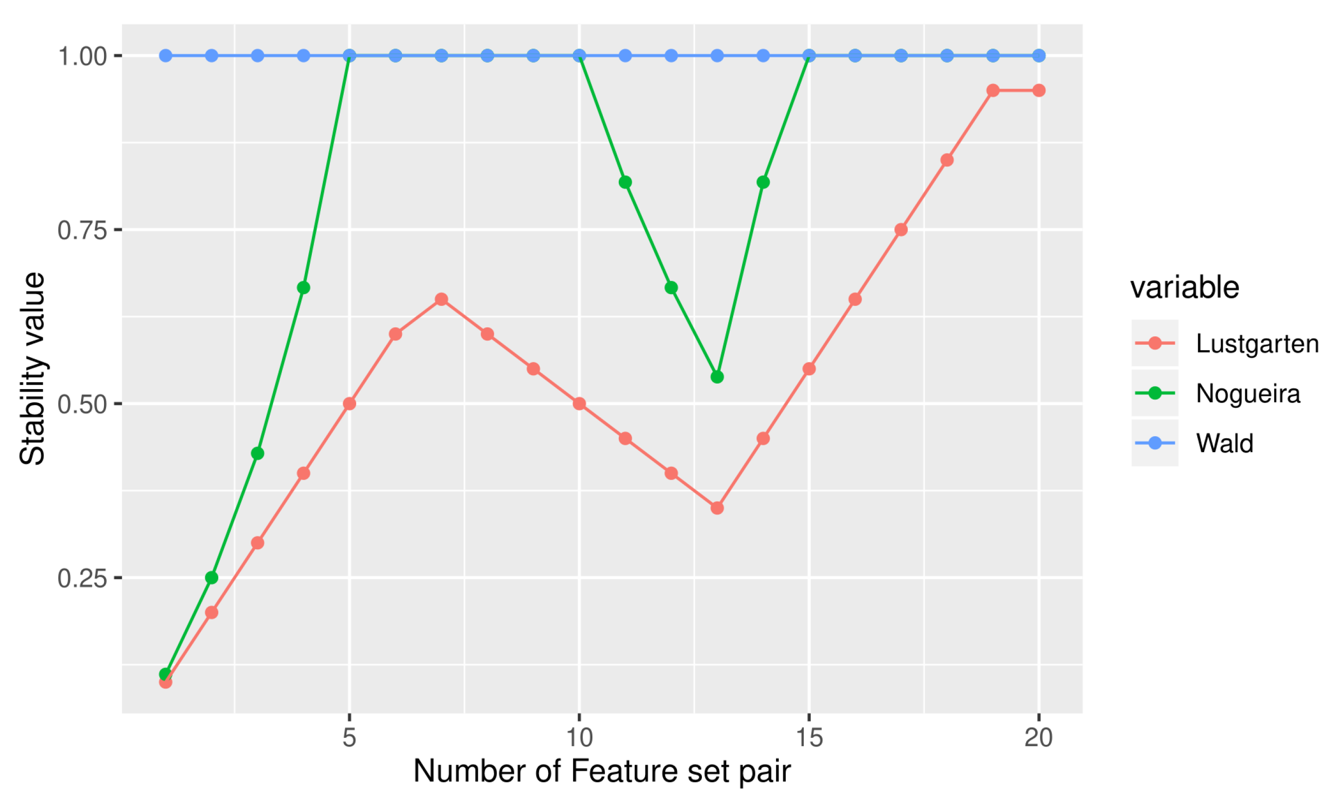
Here we design another experiment for feature subset selection in which each selected feature subset pair consists of two identical feature subsets. The total number of features is same as before, n = 20 and we considered 19 different pairs of the selected feature subsets with different cardinalities.

Table 3. Similarity values for the case when $S_i$ and $S_j$ are identical.

Index of Feature Subset Pair	Cardinality of One Feature Subset ${\mathit{k}}_{\mathit{i}}$	Cardinality of Other Feature Subset ${\mathit{k}}_{\mathit{j}}$	Cardinality of Intersection of Feature Subsets, r	Lustgarten’s Measure, ${\mathit{SI}}_{\mathit{L}}({\mathit{S}}_{\mathit{i}},{\mathit{S}}_{\mathit{j}})$	Nogueira’s Measure, ${\mathit{SI}}_{\mathit{N}}({\mathit{S}}_{\mathit{i}},{\mathit{S}}_{\mathit{j}})$	Wald’s Measure, ${\mathit{SI}}_{\mathit{W}}({\mathit{S}}_{\mathit{i}},{\mathit{S}}_{\mathit{j}})$
1	1	1	1	0.95	1	1
2	2	2	2	0.9	1	1
3	3	3	3	0.85	1	1
4	4	4	4	0.8	1	1
5	5	5	5	0.75	1	1
6	6	6	6	0.7	1	1
7	7	7	7	0.65	1	1
8	8	8	8	0.6	1	1
9	9	9	9	0.55	1	1
10	10	10	10	0.5	1	1
11	11	11	11	0.55	1	1
12	12	12	12	0.6	1	1
13	13	13	13	0.65	1	1
14	14	14	14	0.7	1	1
15	15	15	15	0.75	1	1
16	16	16	16	0.8	1	1
17	17	17	17	0.85	1	1
18	18	18	18	0.9	1	1
19	19	19	19	0.95	1	1

shows the values of the different similarity measures for the case considered here. It is found that as the two stability measures, Nogueira’s measure and Wald’s measure provide the accurate result for similarity calculation as expected. The other measure, Lustgarten’s measure, cannot provide the maximum stability of +1. While Lustgarten’s measure cannot provide the exact value of +1, it provides a value within a known finite range [0.5, +1). The graphical representation of Table 3 is shown in Figure 2. It is noted that Nogueira’s measure provides the same values as the Wald’s measure, resulting overlap of this two lines in the figure. The next experiment has been conducted for the case when the similarity value between two feature subsets is minimal i.e., there is no common feature between the two subsets.

3.

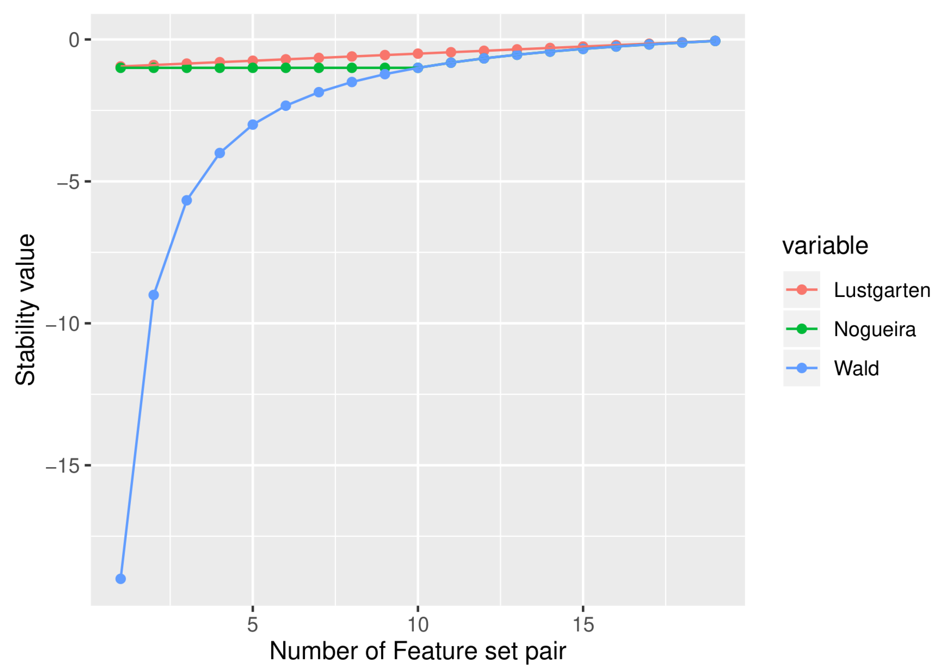
For the case when ${\mathit{S}}_{\mathit{i}}\cap {\mathit{S}}_{\mathit{j}}$ is null ($\mathit{r}=\mathbf{0}$)

As before, the total number of feature in this experiment is, n = 20. We considered 19 different feature subset pairs with the condition $r=0$.

Table 4. Similarity values for the case when $S_i\cap S_j$ is null ($r=0$).

Index of Feature Subset Pair	Cardinality of One Feature Subset ${\mathit{k}}_{\mathit{i}}$	Cardinality of Other Feature Subset ${\mathit{k}}_{\mathit{j}}$	Cardinality of Intersection of Feature Subsets, r	Lustgarten’s Measure, ${\mathit{SI}}_{\mathit{L}}({\mathit{S}}_{\mathit{i}},{\mathit{S}}_{\mathit{j}})$	Nogueira’s Measure, ${\mathit{SI}}_{\mathit{N}}({\mathit{S}}_{\mathit{i}},{\mathit{S}}_{\mathit{j}})$	Wald’s Measure, ${\mathit{SI}}_{\mathit{W}}({\mathit{S}}_{\mathit{i}},{\mathit{S}}_{\mathit{j}})$
1	19	1	0	−0.95	−1	−19
2	18	2	0	−0.9	−1	−9
3	17	3	0	−0.85	−1	−5.67
4	16	4	0	−0.8	−1	−4
5	15	5	0	−0.75	−1	−3
6	14	6	0	−0.7	−1	−2.33
7	13	7	0	−0.65	−1	−1.86
8	12	8	0	−0.6	−1	−1.5
9	11	9	0	−0.55	−1	−1.22
10	10	10	0	−0.5	−1	−1
11	9	9	0	−0.45	−0.82	−0.82
12	8	7	0	−0.4	−0.67	−0.67
13	7	7	0	−0.35	−0.54	−0.54
14	6	6	0	−0.3	−0.43	−0.43
15	5	4	0	−0.25	−0.33	−0.33
16	4	4	0	−0.2	−0.25	−0.25
17	3	2	0	−0.15	−0.18	−0.18
18	2	2	0	−0.1	−0.11	−0.11
19	1	1	0	−0.05	−0.05	−0.05

represents the similarity values of different measures.

It is seen that, in line with the analysis in the previous section, Nogueira’s measure and Wald’s measure reach the minimum value of −1, but does not show the value of −1 for all the cases when r = 0. For Wald’s measure, the minimum value is achieved only when $k_i=k_j=n/2$ with r = 0. The values of Wald’s measure in Table 4 also supports the fact we mathematically proved in the previous section, for example, if $k_i=q$, $k_j=n-q$, $k_i<k_j$ or vice versa, r= 0 and q has the range $q=1,2,3,\cdots n/2$, then Wald’s measure provides the value $(1-n/q)$. Figure 3 represents the graphical view of Table 4. As expected according to our analysis, Nogueira’s stability measure gives the minimal value of −1, for $k_i=q$, $k_j=n-q$, $k_i<k_j$ or vice versa, r = 0 and q has the range $q=1,2,3,\cdots n/2$. For other cases, when $k_i+k_j<n$ and $r=0$, both Nogueira’s measure and Wald’s measure have the same value between −1 and 0. For minimal stability condition, Lustgarten’s measure provides a value between −1 to 0, but never reaches −1.

From the results of the above toy experiments it can be stated that, Lustgarten’s stability measure provides more systematic results than other extended version of Kuncheva index except for two conditions, one is when the two selected feature subsets are identical or stability value should be a fixed maximum value of +1 and another is when intersection between the feature subsets is zero or the stability value should be a fixed minimum value of −1. While the Lustgarten’s stability values in these two cases are not appropriate, the values are bounded by finite numbers. In the next section we propose corrections to the Lustgarten’s measure to make it appropriate for the conditions of maximal and minimal stability. The detail proposal is described in the next section.

5. Proposed Correction of Lustgarten’s Measure

The main shortcomings of Lustgarten’s measure are that it cannot reach its maximum value of +1, when the feature subsets are identical and similarly cannot reach its minimum value of −1 when the cardinality of intersection between feature subsets is zero. Lustgarten’s measure possesses all the desired properties except the property of maximum-minimum value. Here we have proposed corrections to remove the drawbacks.

5.1. Proposed Correction Value for Different Conditions

Different possible cases are considered for correction and are stated below:

• The correction for maximum value:
  The maximum similarity value for the stability measure should occur when the two feature sets are identical, i.e., $k_i=k_j=r$. In this case, Kuncheva index and other stability measures provide the maximum value of +1, but Lustgarten’s measure provides different values which are less than +1, depending on the cardinality of the selected feature subsets. In this work, we propose the correction of the measure based on three different cases for the cardinality of r.
  • Case 1: When $0<r<n/2$
    The Lustgarten’s measure for the feature subsets in this case can be written as:

    $$S{I}_L(S_i,S_j)=\frac{r-\frac{k_i{k}_j}{n}}{min(k_i,k_j)-max(0,k_i+k_j-n)}=\frac{r-\frac{r\ast r}{n}}{r-0}=1-\frac{r}{n}.$$

    where n is the number of all features.
    Correction value = Ideal value − Lustgarten’s measure = $1-(1-\frac{r}{n})=\frac{r}{n}$
  • Case 2: When $r=n/2$
    In this case, Lustgarten’s measure can be written as: -4.6cm0cm

    $$S{I}_L(S_i,S_j)=\frac{r-\frac{k_i{k}_j}{n}}{min(k_i,k_j)-max(0,k_i+k_j-n)}=\frac{r-\frac{n/2n/2}{n}}{r-0}=\frac{n/2-n/4}{n/2}=\frac{1}{2}.$$

    where n is the number of all features.
    Correction value = Ideal value − Lustgarten’s measure = $1-\frac{1}{2}=\frac{1}{2}$
  • Case 3: When $n/2<r<n$
    For this case, Lustgarten’s measure can be written as: -4.6cm0cm

    $$S{I}_L(S_i,S_j)=\frac{r-\frac{k_i{k}_j}{n}}{min(k_i,k_j)-max(0,k_i+k_j-n)}=\frac{r-\frac{r\ast r}{n}}{r-(k_i+k_j-n)}=\frac{r(n-r)}{n(n-r)}=\frac{r}{n}.$$

    where n is the number of all features.
    Correction value = Ideal value − Lustgarten’s measure = $1-\frac{r}{n}=\frac{n-r}{n}$
• The correction for minimum value:
  In this case, selected feature subsets have no common feature, i.e., r = 0. In this condition, Kuncheva index and some other extension of Kuncheva index should provide the minimum value of −1. However, for the Kuncheva index and Wald’s measure, this is satisfied only when $k_i=k_j=k=n/2$. We assessed the correction for the other cases of cardinalities of $k_i$ and $k_j$ as follows:
  • Case 1: When $k_i+k_j=n$.
    In this case, let us consider, $k_i=n-p$ and $k_j=p$, or vice versa, where $p=1,2,3\dots n/2$ Lustgarten’s measure can be written as: -4.6cm0cm

    $$S{I}_L(S_i,S_j)=\frac{r-\frac{k_i{k}_j}{n}}{min(k_i,k_j)-max(0,k_i+k_j-n)}=\frac{0-\frac{p(n-p)}{n}}{p-0}=-\frac{(n-p)}{n}=-\frac{max(k_i,k_j)}{n}$$
    Correction value = Ideal value – Lustgarten’s measure = $-1-(-\frac{max(k_i,k_j)}{n})=\frac{max(k_i,k_j)}{n}-1$
  • Case 2: When $k_i+k_j<n$.
    In this case, let us consider $k_i>k_j$, or vice versa, Lustgarten’s measure can be written as: $S{I}_L(S_i,S_j)=\frac{r-\frac{k_i{k}_j}{n}}{min(k_i,k_j)-max(0,k_i+k_j-n)}=\frac{0-\frac{k_i{k}_j}{n}}{k_j-0}=-\frac{k_i}{n}=-\frac{max(k_i,k_j)}{n}$
    Correction value = Ideal value – Lustgarten’s measure = $-1-(-\frac{max(k_i,k_j)}{n})=\frac{max(k_i,k_j)}{n}-1$
  In all the cases, correction value for the condition $r=0$ is same.

5.2. Proposed Corrected Lustgarten’s Measure

Based on the above analysis, here we summarize our newly proposed corrected Lustgarten’s measure $S{I}_{Lnew}(S_i,S_j)$ in Equation (12) for defining similarity between two selected feature subsets $S_i$ and $S_j$ having cardinalities $k_i$ and $k_j$, respectively, while r, n being the cardinality of intersection of the selected feature subsets and total number of features. In Equation (12), $r=k_i=k_j$, when r is defined within the range $0<r<n$.

$$\begin{array}{c}\hfill S{I}_{Lnew}(S_i,S_j)=\\ \hfill \left\{\begin{array}{cc}\frac{r-\frac{k_i{k}_j}{n}}{min(k_i,k_j)-max(0,k_i+k_j-n)}+\frac{r}{n},\hfill & \mathrm{if}0<r<n/2\hfill \\ \frac{r-\frac{k_i{k}_j}{n}}{min(k_i,k_j)-max(0,k_i+k_j-n)}+\frac{1}{2},\hfill & \mathrm{if}r=n/2\hfill \\ \frac{r-\frac{k_i{k}_j}{n}}{min(k_i,k_j)-max(0,k_i+k_j-n)}+\frac{n-r}{n},\hfill & \mathrm{if}n/2<r<n\hfill \\ \frac{r-\frac{k_i{k}_j}{n}}{min(k_i,k_j)-max(0,k_i+k_j-n)}+\frac{max(k_i,k_j)}{n}-1,\hfill & \mathrm{if}r=0\hfill \\ 0,\hfill & \mathrm{if}r=n\hfill \end{array}\right.\end{array}$$

(12)

5.3. Experiments for Illustration

An experimental illustration have been done, similar to our experiments in the previous section, for verification of the proposed corrected Lustgarten’s measure. As before, the total number of features is $n=20$. Selected feature subset pairs of different cardinalities are considered. Various measures along with our proposed corrected Lustgarten’s measures are used for stability measurement. The results are shown in

Table 5. Comparison of stability measures with proposed corrected Lustgarten’s measure.

Index of Feature Subset Pair	Cardinality of One Feature Subset ${\mathit{k}}_{\mathit{i}}$	Cardinality of Other Feature Subset ${\mathit{k}}_{\mathit{j}}$	Cardinality of Intersection of Feature Subsets, r	Lustgarten’s Measure, ${\mathit{SI}}_{\mathit{L}}({\mathit{S}}_{\mathit{i}},{\mathit{S}}_{\mathit{j}})$	Correction Value in Lustgarten’s Measure	Corrected Lustgarten’s Measure, ${\mathit{SI}}_{\mathit{Lnew}}({\mathit{S}}_{\mathit{i}},{\mathit{S}}_{\mathit{j}})$	Nogueira’s Measure, ${\mathit{SI}}_{\mathit{N}}({\mathit{S}}_{\mathit{i}},{\mathit{S}}_{\mathit{j}})$	Wald’s Measure, ${\mathit{SI}}_{\mathit{W}}({\mathit{S}}_{\mathit{i}},{\mathit{S}}_{\mathit{j}})$
1	1	1	1	0.95	0.05	1	1	1
2	2	2	2	0.90	0.10	1	1	1
3	10	10	10	0.50	0.50	1	1	1
4	19	19	19	0.95	0.05	1	1	1
5	12	12	12	0.60	0.40	1	1	1
6	7	7	7	0.65	0.35	1	1	1
7	19	1	0	−0.95	−0.05	−1	−1	−19
8	15	5	0	−0.75	−0.25	−1	−1	−3
9	10	10	0	−0.50	−0.50	−1	−1	−1
10	5	4	0	−0.25	−0.75	−1	−0.33	−0.33
11	3	2	0	−0.15	−0.85	−1	−0.18	−0.18
12	1	1	0	−0.05	−0.95	−1	−0.05	−0.05
13	18	1	1	0.10	0	0.10	0.11	1
14	10	5	5	0.50	0	0.50	1	1
15	4	12	4	0.40	0	0.40	0.67	1
16	14	3	3	0.30	0	0.30	0.42	1
17	1	10	1	0.50	0	0.50	1	1
18	3	11	3	0.45	0	0.45	0.81	1
19	15	17	15	0.75	0	0.75	1	1
20	9	14	9	0.45	0	0.45	0.81	1

.

In Table 5, the 1st to 6th feature subset pairs are formed in such way that each pair have identical feature subsets, i.e., $k_i=k_j=r$. Corrected Lustgarten’s measure, Nogueira’s and Wald’s measure produce the correct maximum value. For the 7th to 12th feature subset pairs, the intersection between feature subsets for each pair is zero, so the stability should be minimum, with value of −1. Corrected Lustgarten’s measure only provides this minimum stability value for all the feature subset pairs (7th to 12th). For the last eight feature subset pairs (13th to 20th), one feature subset is proper subset of the other feature subset i.e., the two subsets are not identical. Wald’s measure gives a stability value of +1. Nogueira’s measure also gives the stability value of +1 for 3 cases, and less than 1 for rest of the five cases. Lustgarten’s measure produces value less than 1 for all the cases which is more appropriate than Nogueira’s measure or Wald’s measure. It can be verified that corrected Lustgarten’s measure can produce appropriate values in all the different possible cases.

6. Conclusions

Feature selection is a necessary step prior to any classification or mining problem for efficient classification. Stable feature selection algorithm which produce subset of features as unique as possible, is very important for identifying the most relevant and interpretable features for further processing. Stability of any feature selection algorithm refers to its robustness with respect to training set perturbations. Though the idea is simple, its quantification seems challenging. A lot of stability measures for assessment of feature selection algorithms have been proposed so far, but most of them do not follow all the requisite properties of a stability measure.

In this work, at first, we have studied the existing stability measures for evaluation of feature subset selection algorithms and their requisite properties. A leading property, the property of correction for chance, is highlighted and fulfilled by Kuncheva index as a stability measure of feature selection algorithms. However, Kuncheva index is unable to handle variable sizes of feature subsets. To overcome this shortcoming, several modifications and extensions of Kuncheva index are proposed by different researchers. Lustgarten’s measure, Wald’s measure, nPOG and the most recent Nogueira’s measure are the popular measures for stability assessment of feature subset selection algorithms. However, it has been found in our study that none of the measures satisfy all the required properties of a stability measure.

Next, we further investigated Kuncheva index and its modifications and extensions meticulously, highlighting their merits and limitations. We have summarized the required properties of a stability measure and examined whether these are satisfied by the existing popular measures. Finally we have proposed a new modified measure based on the correction of Lustgarten’s stability measure. It is found by toy experiments that, with the proposed new correction, corrected Lustgarten’s measure can overcome the limitations of the other measures and satisfy all the tabulated properties here except the last one which we have not considered in this work. The error in Lustgarten’s stability measure is found to be very specific and systematic compared to erratic behaviour of other extensions of Kuncheva index like Wald’s measure or Nogueira’s measure. So we attempted to correct Lustgarten’s measure to define the new proposed measure and could be able to achieve a new measure which produces consistent values. Stability of a feature selection algorithm can also be considered to have a relationship with the data set. It can be used as a metric for characterization of any data set. We would like to further explore to find out the suitability of any feature subset selection algorithm for a particular data set using our newly proposed measure as a metric.

References

- Brezočnik, L.; Fister, I.; Podgorelec, V. Swarm Intelligence Algorithms for Feature Selection: A Review. Appl. Sci. 2018, 8, 1521. [Google Scholar] [CrossRef] [Green Version]
- Tran, M.Q.; Elsisi, M.; Liu, M.K. Effective feature selection with fuzzy entropy and similarity classifier for chatter vibration diagnosis. Measurement 2021, 184, 109962. [Google Scholar] [CrossRef]
- Tran, M.Q.; Li, Y.C.; Lan, C.Y.; Liu, M.K. Wind Farm Fault Detection by Monitoring Wind Speed in the Wake Region. Energies 2020, 13, 6559. [Google Scholar] [CrossRef]
- Tran, M.Q.; Liu, M.K.; Elsisi, M. Effective multi-sensor data fusion for chatter detection in milling process. ISA Trans. 2021. [Google Scholar] [CrossRef] [PubMed]
- Cilia, N.D.; De Stefano, C.; Fontanella, F.; Raimondo, S.; Scotto di Freca, A. An Experimental Comparison of Feature-Selection and Classification Methods for Microarray Datasets. Information 2019, 10, 109. [Google Scholar] [CrossRef] [Green Version]
- Turney, P. Technical Note: Bias and the Quantification of Stability. Mach. Learn. 1995, 20, 23–33. [Google Scholar] [CrossRef] [Green Version]
- Stiglic, G.; Kokol, P. Stability of ranked gene lists in large microarray analysis studies. J. Biomed. Biotechnol. 2010, 2010. [Google Scholar] [CrossRef] [PubMed] [Green Version]
- Levner, I. Feature selection and nearest centroid classification for protein mass spectrometry. BMC Bioinform. 2005, 6, 68. [Google Scholar] [CrossRef] [PubMed] [Green Version]
- Zhang, K.; Qin, Z.S.; Liu, J.S.; Chen, T.; Waterman, M.S.; Sun, F. Haplotype block partitioning and tag SNP selection using genotype data and their applications to association studies. Genome Res. 2004, 14, 908–916. [Google Scholar] [CrossRef] [Green Version]
- Kalousis, A.; Prados, J.; Hilario, M. Stability of feature selection algorithms: A study on high-dimensional spaces. Knowl. Inf. Syst. 2007, 12, 95–116. [Google Scholar] [CrossRef] [Green Version]
- Kuncheva, L.I. A stability index for feature selection. In Proceedings of the 25th IASTED International Multi-Conference: Artificial Intelligence and Applications, Innsbruck, Austria, 13–15 February 2007; pp. 390–395. [Google Scholar]
- Khaire, U.M.; Dhanalakshmi, R. Stability of feature selection algorithm: A review. J. King Saud Univ.-Comput. Inf. Sci. 2019. [Google Scholar] [CrossRef]
- Mohana Chelvan, P.; Perumal, K. A survey on feature selection stability measures. Int. J. Comput. Inf. Technol. 2016, 5, 98–103. [Google Scholar]
- Dunne, K.; Cunningham, P.; Azuaje, F. Solutions to instability problems with sequential wrapper-based approaches to feature selection. J. Mach. Learn. Res. 2002, 1–22. [Google Scholar]
- Nogueira, S.; Sechidis, K.; Brown, G. On the stability of feature selection algorithms. J. Mach. Learn. Res. 2018, 18, 6345–6398. [Google Scholar]
- Kalousis, A.; Prados, J.; Hilario, M. Stability of feature selection algorithms. In Proceedings of the Fifth IEEE International Conference on Data Mining (ICDM’05), Houston, TX, USA, 27–30 November 2005; p. 8. [Google Scholar]
- Yu, L.; Han, Y.; Berens, M.E. Stable gene selection from microarray data via sample weighting. IEEE/ACM Trans. Comput. Biol. Bioinform. 2011, 9, 262–272. [Google Scholar]
- Yu, L.; Ding, C.; Loscalzo, S. Stable feature selection via dense feature groups. In Proceedings of the 14th ACM SIGKDD International Conference on Knowledge Discovery and Data Mining, Las Vegas, NV, USA, 24–27 August 2008; pp. 803–811. [Google Scholar]
- Zucknick, M.; Richardson, S.; Stronach, E.A. Comparing the characteristics of gene expression profiles derived by univariate and multivariate classification methods. Stat. Appl. Genet. Mol. Biol. 2008, 7. [Google Scholar] [CrossRef]
- Zhang, M.; Yao, C.; Guo, Z.; Zou, J.; Zhang, L.; Xiao, H.; Wang, D.; Yang, D.; Gong, X.; Zhu, J.; et al. Apparently low reproducibility of true differential expression discoveries in microarray studies. Bioinformatics 2008, 24, 2057–2063. [Google Scholar] [CrossRef] [Green Version]
- Lee, K.E.; Sha, N.; Dougherty, E.R.; Vannucci, M.; Mallick, B.K. Gene selection: A Bayesian variable selection approach. Bioinformatics 2003, 19, 90–97. [Google Scholar] [CrossRef]
- Yeung, K.Y.; Bumgarner, R.E.; Raftery, A.E. Bayesian model averaging: Development of an improved multi-class, gene selection and classification tool for microarray data. Bioinformatics 2005, 21, 2394–2402. [Google Scholar] [CrossRef] [Green Version]
- Dutkowski, J.; Gambin, A. On consensus biomarker selection. BMC Bioinform. 2007, 8, S5. [Google Scholar] [CrossRef] [PubMed] [Green Version]
- Yang, Y.H.; Xiao, Y.; Segal, M.R. Identifying differentially expressed genes from microarray experiments via statistic synthesis. Bioinformatics 2005, 21, 1084–1093. [Google Scholar] [CrossRef] [Green Version]
- Abeel, T.; Helleputte, T.; Van de Peer, Y.; Dupont, P.; Saeys, Y. Robust biomarker identification for cancer diagnosis with ensemble feature selection methods. Bioinformatics 2010, 26, 392–398. [Google Scholar] [CrossRef]
- Davis, C.A.; Gerick, F.; Hintermair, V.; Friedel, C.C.; Fundel, K.; Küffner, R.; Zimmer, R. Reliable gene signatures for microarray classification: Assessment of stability and performance. Bioinformatics 2006, 22, 2356–2363. [Google Scholar] [CrossRef] [Green Version]
- Duan, K.B.; Rajapakse, J.C.; Wang, H.; Azuaje, F. Multiple SVM-RFE for gene selection in cancer classification with expression data. IEEE Trans. Nanobiosci. 2005, 4, 228–234. [Google Scholar] [CrossRef]
- Lustgarten, J.L.; Gopalakrishnan, V.; Visweswaran, S. Measuring stability of feature selection in biomedical datasets. In AMIA Annual Symposium Proceedings; American Medical Informatics Association: Bethesda, MD, USA, 2009; Volume 2009, p. 406. [Google Scholar]
- Khoshgoftaar, T.M.; Fazelpour, A.; Wang, H.; Wald, R. A survey of stability analysis of feature subset selection techniques. In Proceedings of the 2013 IEEE 14th International Conference on Information Reuse & Integration (IRI), San Francisco, CA, USA, 14–16 August 2013; pp. 424–431. [Google Scholar]
- Wald, R.; Khoshgoftaar, T.M.; Napolitano, A. Stability of filter-and wrapper-based feature subset selection. In Proceedings of the 2013 IEEE 25th International Conference on Tools with Artificial Intelligence, Herndon, VA, USA, 4–6 November 2013; pp. 374–380. [Google Scholar]
- Zhang, M.; Zhang, L.; Zou, J.; Yao, C.; Xiao, H.; Liu, Q.; Wang, J.; Wang, D.; Wang, C.; Guo, Z. Evaluating reproducibility of differential expression discoveries in microarray studies by considering correlated molecular changes. Bioinformatics 2009, 25, 1662–1668. [Google Scholar] [CrossRef]
- Nogueira, S.; Brown, G. Measuring the stability of feature selection with applications to ensemble methods. In International Workshop on Multiple Classifier Systems; Springer: Cham, Switzerland, 2015; pp. 135–146. [Google Scholar]
- Nogueira, S.; Brown, G. Measuring the stability of feature selection. In Joint European Conference on Machine Learning and Knowledge Discovery in Databases; Springer: Cham, Switzerland, 2016; pp. 442–457. [Google Scholar]