
Graph-Based Siamese Network for Authorship Verification
by
 ,
,
Daniel Embarcadero-Ruiz
1, 
Helena Gómez-Adorno
2,* ,
,
Alberto Embarcadero-Ruiz
1 and
Gerardo Sierra
3 1
Posgrado en Ciencia e Ingeniería de la Computación, Universidad Nacional Autónoma de México, Mexico City 04510, Mexico
2
Instituto de Investigaciones en Matemáticas Aplicadas y en Sistemas, Universidad Nacional Autónoma de México, Mexico City 04510, Mexico
3
Instituto de Ingeniería, Universidad Nacional Autónoma de México, Mexico City 04510, Mexico
*
Author to whom correspondence should be addressed.
Mathematics 2022, 10(2), 277; https://0-doi-org.brum.beds.ac.uk/10.3390/math10020277
Submission received: 1 December 2021
/
Revised: 8 January 2022
/
Accepted: 11 January 2022
/
Published: 17 January 2022
(This article belongs to the Special Issue Graphs, Metrics and Models)
Abstract
:In this work, we propose a novel approach to solve the authorship identification task on a cross-topic and open-set scenario. Authorship verification is the task of determining whether or not two texts were written by the same author. We model the documents in a graph representation and then a graph neural network extracts relevant features from these graph representations. We present three strategies to represent the texts as graphs based on the co-occurrence of the POS labels of words. We propose a Siamese Network architecture composed of graph convolutional networks along with pooling and classification layers. We present different variants of the architecture and discuss the performance of each one. To evaluate our approach we used a collection of fanfiction texts provided by the PAN@CLEF 2021 shared task in two settings: a “small” corpus and a “large” corpus. Our graph-based approach achieved average scores (AUC ROC, F1, Brier score, F0.5u, and C@1) between 90% and 92.83% when training on the “small” and “large” corpus, respectively. Our model obtain results comparable to those of the state of the art in this task and greater than traditional baselines.
1. Introduction
Authorship analysis aims to identify characteristics of an author’s writing style given a text sample, and ultimately to identify the author himself. The idea behind this research area is that some features of the documents allow distinguishing texts written by different authors [1].
There are different tasks in authorship analysis; for example, authorship attribution, author profiling, author clustering, and plagiarism detection [2]. The authorship verification task aims to determine if two given texts were written by the same author. We focus our research on an open-set scenario, i.e., the model will be evaluated on a dataset that has texts which authors never seen in the training dataset.
The main contribution of this work is a novel Siamese network architecture composed of two graph convolutional neural networks, pooling, and classification layers to approach the authorship verification task. We present three strategies (short, med, and full) for representing texts as graphs based on the relation of the POS labels and co-occurrence of the words. Each strategy varies in the complexity of the graph and the computational cost for processing it. Our motivation is that graph representation provides structural information that is not available when texts are processed in the traditional sequential manner.
In the first part of this paper, we present experiments varying the graph convolutional layers and the number of layers in pooling and classification, for each graph representations used. Later, we propose combining more than one graph-based representation for the feature extraction in an ensemble architecture. We add a stylistic-based feature extraction component to the Siamese Network architecture to improve the performance of the models. For this ensemble architecture, we present the evaluation of different training strategies. Finally, we present a technique for a threshold adjustment that improves the performance of our architectures on the authorship verification task.
The rest of this paper is organized as follows. Section 2 presents an overview of the literature on authorship verification. Section 3.1 includes the description of the dataset used to evaluate our approach. The details of the process to model texts on graphs are presented in Section 3.2 and our Graph-based Siamese network is explained in Section 3.3. The ensemble architecture is presented in Section 3.4. Section 4 reports and analyzes the results obtained by the different experiments with the proposed architectures and baseline methods. In particular, in Section 4.5 we present the comparison of our method with some state of the art methods in the context of the Authorship Verification shared task at PAN 21 (https://pan.webis.de/, accessed on 21 July 2020). Finally, Section 5 presents our conclusions and points out future research lines.
2. Related Work
The formal study of authorship analysis started in the 19th century, it was first tackled with linguistic approaches and eventually by statistical and computational methods [3]. These tasks continue to grow attention for their practical applications; for example, in a variety of computer crime investigations ranging from homicide to identity theft and many types of financial crimes [4] or in the context of identifying the author of source code [5].
In general, the most popular approach for authorship analysis is to extract features from the texts and use them to train a classification algorithm, which can be based either trained on supervised learning or similarimeasures. We can distinguish the extracted features according to the computational requirements for extracting them in lexical-level—i.e., word length, sentence length, bag of words, vocabulary richness, misspelled words; character-level—i.e., character n-grams, character types, count of special characters; syntactic-level—i.e., POS tags, chunks, sentence and phrase structure; and semantic-level—i.e., semantic dependencies, synonyms [2].
Some supervised classification algorithms used in authorship verification tasks are support vector machines, decision trees, discriminant analysis, neural networks, and genetic algorithms [6]. Another option is to calculate the similarity between texts and use it to predict whether both texts are written by the same author or not; this is a more natural approach if we take authorship verification as an open set classification problem over a lot of possible authors [7].
A specifically designed solution for the authorship verification task is the unmasking method, proposed by [8]. This method tries to measure how deep the difference is between two texts by comparing them several times (iterations), each time one using fewer relevant features. This method achieved an accuracy of 95.7% when tested on datasets of long texts of about 500 K words. When trying to apply it to datasets of shorter texts or texts of a different genre and topics the performance decreased considerably. For example, Kestemont et al. [9] evaluates the performance of the unmasking method over a dataset of theatrical and prose texts of about 10,000 words obtaining an accuracy of just 77%.
Bevendorff et al. [10] proposed an alternative unmasking method that obtains an accuracy between 75% and 80% on short texts of about 4000 words. The performance of the original unmasking method hinges on the availability of sufficiently many paragraphs per text, each one of enough length. If the paragraphs are too short, the training data becomes too sparse and no descriptive curves can be generated. The authors exploit the bag-of-words nature of the unmasking features and create the paragraphs by oversampling words in a bootstrap aggregating manner.
Another relevant strategy to tackle the authorship verification task is the impostors’ method [7,11]. This method proposes using a set of impostor documents collected from an outsource (usually the web) in a way that these impostor documents have a similar topic with the known and unknown document. A set of features are also defined, some of the features included in this set are function words, word n-grams, and character n-grams.
Before 2015, the authorship verification task was mainly evaluated using datasets on training and testing documents that shared the same topic and same genre. It was observed that in a cross-topic scenario the performance of the traditional approaches decreases [12].
Stamatatos [13] showed that the character n-grams are more reliable than other lexical features for the authorship analysis task when the genre and topic of the documents vary. Sapkota et al. [14] claimed that some kind of n-grams work better than others as features for classification. In particular, some trigrams that include punctuation marks work better in a cross-topic scenario.
The use of a heterogeneous classifier that combines independent classifiers each one with a different approach has achieved good results, usually better than the ones obtained using a single classifier [6,12]. PAN is a series of scientific events and shared tasks on digital text forensics and stylometry (https://pan.webis.de/, accessed on 21 July 2020). Since 2011, it focused on authorship analysis tasks and the methods presented in their workshops are the state of the art in this research area [15].
In recent years, neural network architectures have been proposed to solve the task. For example, Bagnall [16] proposed a recurrent neural network architecture over characters to solve the authorship verification task in the PAN 2015 dataset. This approach achieved considerably better results than other approaches over the same dataset but it is computationally more expensive.
Jafariakinabad et al. [17] introduced a syntactic recurrent neural network to encode the syntactic patterns of a document in a hierarchical structure. The model first learns the syntactic representation of sentences from the sequence of POS tags. Their experimental results on the PAN 2012 dataset for the authorship attribution task show that the syntactic recurrent neural network (working over POS tag embeddings) outperforms the lexical model (working over word embeddings) with an identical architecture by approximately 14% in terms of accuracy.
Weerasinghe and Greenstadt [18] proposed a model with notable performance using a stylometric approach. They extracted stylometric features from each text pair and used the absolute differences between the feature vectors as input to a classifier. They evaluated one model using a logistic regression classifier and another using a neural network approach.
2.1. Graph-Based Representation of Texts
A common and standard approach to model text documents is bag-of-words. This model is suitable for capturing word frequency; however, structural and semantic information is ignored. Graph representation is a mathematical construct and can model relationships and structural information effectively. A text can be appropriately represented as a graph using feature term as vertices and significant relations between the feature terms as edges [19].
There are several graph-based representations used to model documents. The general approach consists of identifying relevant elements in the text—i.e., words, sentences, paragraphs, etc.—and considering them as nodes in the graph. Then meaningful relations between these elements are considered to be edges. Traditionally, the elements used as nodes in the graph are words, sentences, paragraphs, documents, and concepts. To define the edges, usually syntactic, semantic relations, and statistical counts are used [19].
Some relevant graph-based representations proposed for a variety of authorship analysis tasks are: co-occurrence graph, co-occurrence based on POS, semantic graph and hierarchical keyword graph [19]. Pinto et al. [20] present another graph-based approach for document understanding. In this work, the authors proposed representing texts as Integrated Syntactic Graphs (ISG). This approach considers different levels of linguistic analysis, such as lexical, morphological, syntactical, and semantic, to build a graph representation of a given document. The authors also introduce a technique for extracting useful text patterns based on shortest paths.
Castillo et al. [21] present an overview of different graph-based representations proposed to solve authorship analysis tasks. The aim of this manuscript is to highlight the importance of enriched vs. non-enriched co-occurrence graphs as an alternative to traditional feature representation models such as vector representation. In particular, in [22], the authors applied the proposed graph-based approach on the English language partitions of the CLEF PAN 2014 and 2015 Authorship Verification datasets, reporting competitive results that outperform the baseline used in the PAN 2014 Authorship Verification shared task. They proposed using four centrality measures: closeness, betweenness, degree, and eigenvector to detect relevant patterns of an author’s writing style. In particular, they found that words with a high closeness which is part of some chunk phrases and words with high betweenness that are included in bigrams and trigrams, contribute in a more effective way to verify document authorship.
Gómez-Adorno et al. [23] generalize the graph-based method described in [20], initially proposed for the extraction of text patterns obtained by shortest path traversal over Integrated Syntactic Graphs (ISG). They build the ISG representation using linguistic features of various levels of language description, which provides relevant information about the texts. In particular, they show that their method discovers patterns that can be used in authorship attribution and authorship verification.
2.2. Graph Neural Networks
There is an increasing number of applications where data can be naturally represented in the form of graphs. While deep learning effectively captures hidden patterns of Euclidean data, graph neural networks can help us to generalize the deep learning approach to data represented as graphs [24].
There exist just a couple of works that applied Graph Neural Networks techniques to an Authorship analysis task. For instance, Cruz [25] evaluate the robustness of three different approaches for the Authorship Attribution task when the length of the text is varied from 2500 to 20,000 tokens. The first two tested approaches are a global strategy and a local strategy based on complex network measurements. The third approach tested is a graph embedding technique based on a skip-gram model called Graph2Vec [26]. They found that the local strategy with linear discriminant analysis achieves 97% of accuracy and conclude that it is better to describe short texts than Graph2Vec with low dimension. However, the performance on local and global strategies decreases while the length of each text is increasing, in contrast to the graph embedding technique, which has better results with the large length of texts. A relevant note about these results is that they remove all punctuation marks, remove language stop-words and use lemmatization.
In [27], the authors consider a task from traditional literary criticism: annotating a structured, composite document with information about its sources, and approach it as an Authorship Attribution task. They take the Documentary Hypothesis, a prominent theory regarding the composition of the first five books of the Hebrew bible, extract stylistic features designed to avoid bias or overfitting and train several classification models over the source labels assigned in each part of the texts. Their main result is that the graph convolutional network architecture outperforms structurally uninformed models.
2.3. Siamese Neural Networks
Siamese Neural Networks (SNN) was first presented by Bromley et al. [28] to solve the problem of signature verification. Their formulation defines two separate sub-networks, each one acting on an input pattern to extract features. The key idea of their formulation is that the two sub-networks share their weight; that means that both sub-networks must extract the features exactly in the same way. They use the cosine of the angle between the two feature vectors obtained by the sub-networks to assign a distance between the compared instances. The idea is that the siamese network learn how to extract feature vectors from the instances in a way these vectors are close if the instances are similar and these vectors are far if not. SNNs are in general computationally expensive but perform better as compared to other techniques when learning similarity [29].
Koch et al. [30] proposed a Siamese convolutional network to solve face verification, they emphasize the application of their architecture to manage the one-shot recognition problem. Furthermore, instead of using a contrastive loss as the objective loss, they use a fully connected layer followed by a sigmoid function on top of the Siamese network to obtain a prediction and optimize a cross-entropy loss with normalization.
Recently, SNNs were proposed to solve the authorship verification task. For instance, two approaches used SNNs to solve the PAN Authorship 2020 Verification Task.
Boenninghoff et al. [31] used a Siamese architecture of LSTMs with attention coefficients to extract first sentence embeddings and after that a document embedding. This Siamese network aims to learn a pseudo-metric that maps a document of variable length onto a fixed-sized feature vector. At the top, they also incorporate a probabilistic layer to perform Bayes factor scoring in the learned metric space. In their model, they incorporate some text preprocessing strategies such as topic masking, using a sliding window to generate the sentences, and data augmentation. Their proposed method achieved excellent overall performance scores, outperforming all other systems that participated in the PAN 2020 Authorship Verification Task, in both the small and “large” datasets.
Araujo-Pino et al. [32] used a Siamese neural network approach that receives as input the character n-gram representation (with n varying from 1 to 3) of the document pairs to be compared.
We can conclude that modeling texts as graphs is a natural way to take advantage of the structural information contained in the text. Furthermore, several graph-based representations of texts showed good results in the Authorship Analysis task, but we notice that the known graph-based approaches usually introduce particular techniques to extract relevant vector features, that are dependent on the application. The Graph Neural Network approach is a way to allow a model to learn relevant patterns from the data instead of proposing hand-crafted methods to extract features.
The Siamese Neural Network was successfully applied to track several verification-related tasks. We found two relevant approaches used for the Authorship Verification task, but both approaches model the texts in a sequential manner. We consider that using Graph Neural Networks to extract relevant patterns automatically as part of a Siamese Neural Network architecture is a natural and powerful way to take advantage of a graph-based representation of texts.
3. Materials and Methods
In this section, we describe the datasets used to evaluate our methodology and a detailed description of our proposed methods. As a core part of our method, we describe the graph modeling from texts in detail in Section 3.2.
3.1. Datasets
We used the training datasets provided by PAN@CLEF for the Authorship Verification task 2021 [33]. We will refer to these datasets as “small” and “large” according to their size. Table 1 shows basic statistics of both datasets; the first column shows many pairs of texts (problems) each dataset has, the other columns show how many different texts, authors, and topics are included in each dataset.
Each problem is composed of two fanfiction texts; fanfiction is a story originally written by a fan that extends the universe of a fandom topic. All texts are written in English, which have an average of 21,400 characters, 4950 tokens and 345 sentences.
We cleaned each dataset by removing texts with less than 200 tokens (which are meaningless texts) and also by removing duplicated pairs of texts that appear in the original datasets with different problem ids. In total, we just remove 6 problems from the “small” dataset and 19 problems from the “large” dataset.
We split the dataset into three parts: train, validation, and test. We trained our models on the train split, using the validation split to calibrate the hyperparameters, and used the test split to obtain a reference score of the model. We did not use any of the samples in the test split to calibrate our model, so the score in this set tells us about the generalization ability of the model. Our splits were done using the same fixed pairs given by the dataset. We made these splits author disjoint, i.e., no text in one split has the same author as another text in a different split. In particular, all the texts in the test split have authors never seen by the model during the training step. There are shared topics between these splits, we did not make our splits topic disjoint.
All the splits were defined with a balanced proportion of true and false problems. Table 2 shows the total number of problems and the number of problems in the positive class (those problems belonging to the same author) on our splits.
3.2. Modeling Texts as Graphs
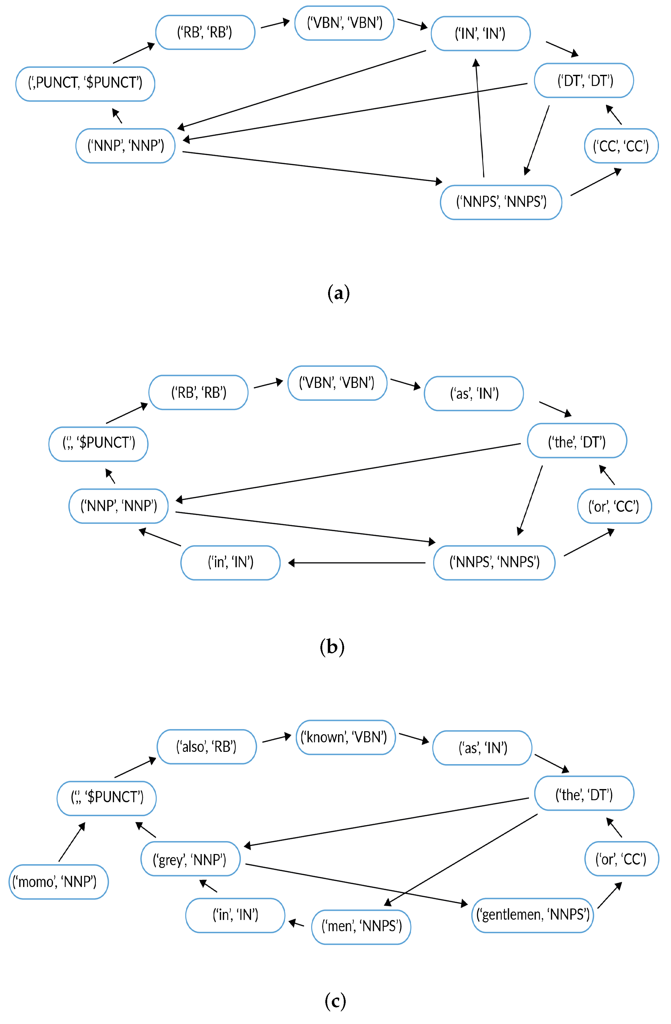
A core component of our method corresponds to the modeling of the texts as graphs. Our graph representation attempts to capture the relationships between words and POS labels in the text. To make clear our process we use the next text as an example:
Momo, also known as The Grey Gentlemen or The Men in Grey, First, each text is preprocessed as follows:
- Substitute non-ASCII characters to ASCII equivalent. We employed the unidecode package (https://github.com/avian2/unidecode, accessed on 21 July 2021).
- Tokenize and obtain the POS label.
- Lowercasing.
We do not remove punctuation of any type, the non-ASCII character substitution was made to reduce the variability of the used punctuation.
To obtain the POS labels, we considered the PENN-Treebank POS labels [34] obtained by the NLTK package (https://www.nltk.org, accessed on 5 January 2022) and after that, we add two additional labels: $PUNCT to mark all punctuation and $OTHER to mark any other word that the NLTK model failed to identify. In total, we consider 38 labels. After this process we obtain a parsed text like this:
| [ | (‘momo’, ‘NNP’), (‘,’, ‘$PUNCT’), (‘also’, ‘RB’), (‘known’, ‘VBN’), |
| (‘as’, ‘IN’), (‘the’, ‘DT’), (‘grey’, ‘NNP’), (‘gentlemen’, ‘NNP’), | |
| (‘or’, ‘CC’), (‘the’, ‘DT’), (‘men’, ‘NNPS’), (‘in’, ‘IN’), | |
| (‘grey’, ‘NNP’), (‘,’, ‘$PUNCT’)] |
We construct a directed graph based on a co-occurrence graph, as explained in [19] but with a different edge weighting. We consider that two words co-occur if them appear right next to each other in the text. We used the Networkx (https://networkx.org/, accessed on 21 July 2021) package to construct the graphs. We define the graph as an ordered pair , where V is a set of vertices composed by tuples and E is a set of weighted edges. The edge set , where w is the edge weight.
We define a set of POS labels and denote it as REDUCE_LABELS. In the construction, we identify all tuples from parsed text with a label in the REDUCE_LABELS set as a single node. With this, the graph structure changes and also the information abstracted from the text. To construct the graph, let P be the parsed text as a list of tuples, the number of elements in the list, and the i-th element in the list. For each in P, we can define:
where M is the list defined by the tuples masked as explained. For each pair of tuples let be the number of times is followed by in M and let be ; note that T is the total number of times a pair of tuples co-occur in M.
Now we can define the nodes and edges of our graph:
Please note that M is a list with order and V is just the set of all tuples in M. We want to define an edge between any two nodes (tuples) that appear together in the list M:
As we said before, with this construction we identify all tuples with a specific label in the REDUCE_LABELS set as a single node. In our experiments, we evaluated graphs generated with different REDUCE_LABELS sets. From now we will denominate short graph to the graph generated using the set of all possible POS labels as REDUCE_LABELS, full graph to the graph generated using REDUCE_LABELS and we will denominate med graph to the graph generated using the following set of REDUCE_LABELS:
| REDUCE_LABELS = [ | ‘JJ’, ‘JJR’, ‘JJS’, | # Adjectives |
| ‘NN’, ‘NNS’, ‘NNP’, ‘NNPS’, | # Nouns | |
| ‘RB’, ‘RBR’, ‘RBS’, | # Adverbs | |
| ‘VB’, ‘VBD’, ‘VBG’, | # Verbs | |
| ‘VBN’,‘VBP’, ‘VBZ’, | # Verbs | |
| ‘CD’, | # Cardinal numbers | |
| ‘FW’, | # Foreign words | |
| ‘LS’, | # List item marker | |
| ‘SYM’, | # Symbols | |
| ‘$OTHER’ | # Others] |
The size of the graph depends on the REDUCE_LABELS set used in the construction. In Table 3, we include the average number of nodes and edges of each graph construction over all the texts used in the “large” dataset for the PAN 2021 Authorship Verification task; as a reference, each text has an average of 4950 tokens.
Continuing with our example, the short graph, the med graph and the full graph are showed in Figure 1a–c, respectively; for simplicity we do not draw the edge weights.
To input our graph to a neural network, we need to encode each node into a vector. To that end, we use a one-hot encoding representation with respect to the 38 possible POS labels used. We chose to consider only the POS tag information because of two reasons: There exist references where a deep learning model training over POS embeddings instead of word embeddings obtain better results for an authorship analysis task [17]. Furthermore, using low dimension POS embeddings to represent nodes instead of word embeddings of larger dimension, allows us to reduce the computational cost of the model. The results obtained with these decision are comparable with models based on word embeddings, as we can see in [33].
In the final graph, each node is represented by a vector of dimension 38 that encodes their POS label.
3.3. Graph-Based Siamese Network (GBSN)
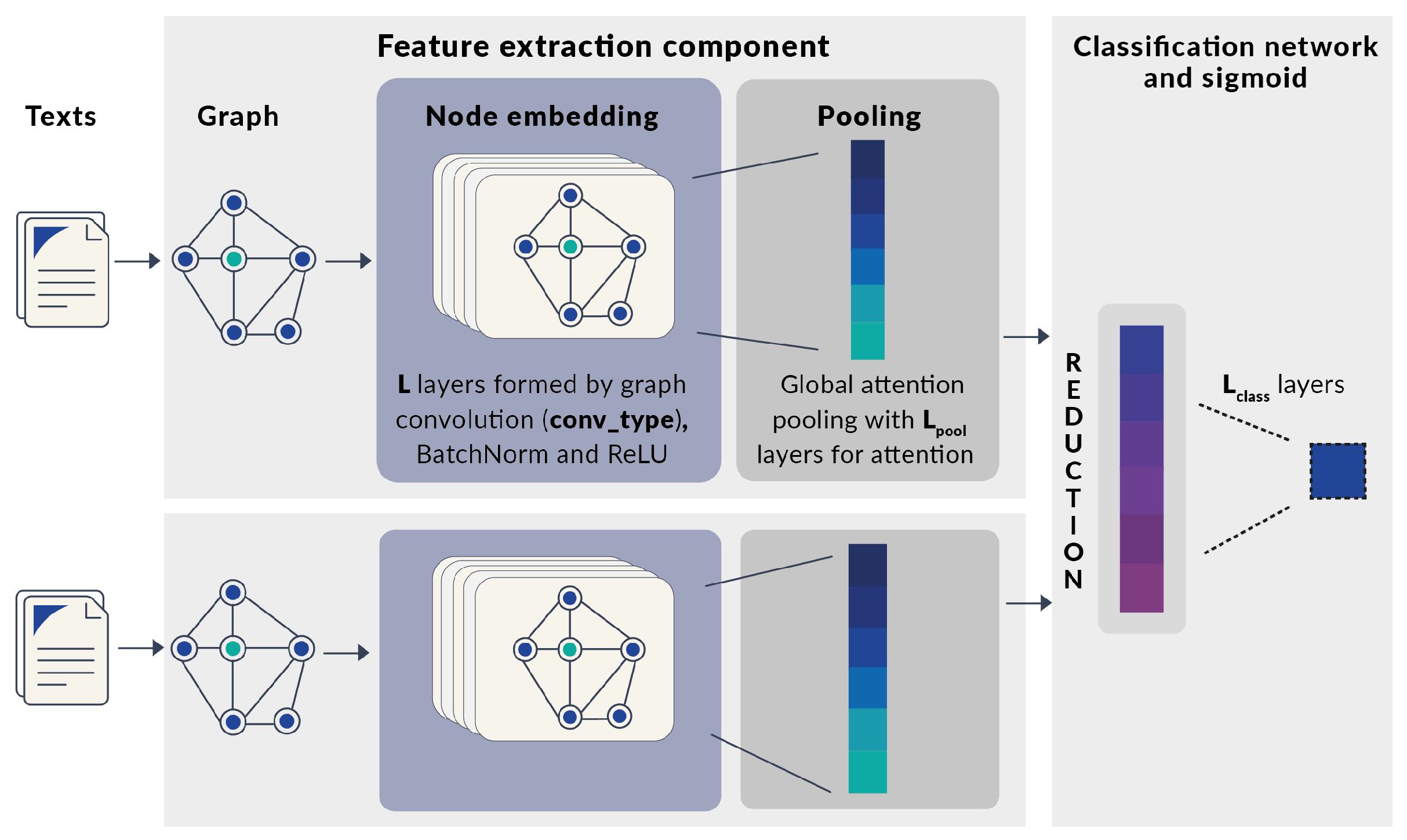
To approach the authorship verification task, we use a Siamese network architecture [28] including a component to transform texts as co-occurrence graphs. Our Graph-based Siamese network (Figure 2) is composed of two identical feature extraction components with shared weights, a reduction step, and a classification network.
Each feature extraction component receives a text, transforms it into a graph, and returns a vector representation of this graph; the objective is to extract relevant features that can identify the author’s style from the graph representation of the texts. We can distinguish three parts in the feature extraction component: graph representation, node embedding layers, and global pooling.
In our architecture, a node embedding layer is composed of a graph convolutional layer, followed by a batch normalization layer, and a ReLU (Rectified linear activation function). We will call to the parameter identifying the graph convolutional layer type and L to the parameter identifying the amount of node embedding layers used by the architecture.
The first node embedding layer takes as input a graph with an initial feature vector in each node; as we described in Section 3.2 each initial node vector has dimension 38 because this vector is a one-hot representation of the POS label of the node. The output of each node embedding layer is the same graph structure with new feature vectors in each node; the dimension of the vectors obtained can be defined in the same way we define the channels used in a traditional convolutional layer. Our architecture obtains vectors of dimension 64 in each convolutional layer.
For the parameter we use the convolutional layers proposed to learn features from nodes, that also take into account the edge weights in their formulation. All the selected layers were used as implemented in PyTorch-geometric (https://pytorch-geometric.readthedocs.io/en/latest/, accessed on 21 July 2021) with the default parameters when no other choice is explicitly described here:
- GraphConv: A basic implementation of the graph neural network model described by Morris et al. [35].
- LEConv: Originally proposed by Ranjan et al. [36] to select relevant clusters in a graph, the authors prove that it is more expressive than other layers such as the Graph Convolutional Network layer as defined by Kipf and Welling [37] and affirm it can consider both local and global importance of nodes.
- GCN2Conv: The Graph Convolutional Network via initial residual and identity mapping proposed in [38]. This layer was proposed to solve the over-smoothing problem by including a skip connection to the input layer. We implemented this layer with parameter .
- TAGConv: The Topology Adaptive Graph Convolutional network proposed by Du et al. [39]. This layer is defined in a way that in just one layer it can see the information of not just consecutive nodes but nodes at distance K. We performed our experiments with the default .
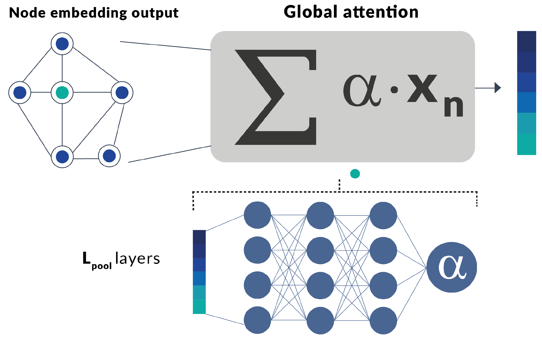
We need a pooling layer to obtain a single vector representation for the whole graph. This layer needs to be capable of receiving a graph with any number of nodes and structure. Pooling layers based on the sum, average or maximum value of the vectors in each node had been use in several graph classification tasks because of its simpleness [24]. To be a step forward, we chose to use a pooling layer that not just sum the values, but perform attention over them. The soft attention allows the model to consider the nodes accordingly to its feature vector. With these, we expect that this layer will be able to compute a more accurate and useful graph representation.
In our model, we use a global attention layer for the pooling, originally proposed by Li et al. [40]. As it is shown in Figure 3, this layer takes the final output of the node feature extraction component as its input, i.e., a graph with the vector embedding in each node. To obtain the final vector, it makes a weighted sum of each node vector with a coefficient obtained by doing attention over these same vectors, the formulation is:
where V is the set of all nodes in the graphs and h is a fully connected neural network with a single scalar as output. This fully connected neural network has ReLU (Rectified linear activation function) activation, 32 neurons in each hidden layer, and total layers. The final output of each feature extraction component is a vector with dimension 64.
For the reduction step, we simply compute the absolute value of the difference between the output of each feature extraction component for each document to be verified. The resulting vector is passed to a final classification network. The classification network is a fully connected network with ReLU (Rectified linear activation function) activation, 64 neurons in each hidden layer, total layers, and a final sigmoid function.
Our model returns a single value in the interval that can be interpreted as a measure of how much the two submitted texts are alike. An output close to 1 tells us that the model finds both texts to be from the same author. To evaluate our models, we use as default a threshold of , i.e., if the output is higher than the model says both texts are from the same author, if it is lower than both texts are from different authors and if it is exactly the model does not answer this problem.
3.4. GBSN Ensemble Architecture
We upgrade our base architecture putting side by side different feature extraction components in a new Graph-based Siamese Network Ensemble architecture. Each subnetwork in the Siamese architecture is now formed by several independent feature extraction components, each obtaining a vector from the text, as shown in Figure 4.
We proposed two types of feature extraction components: the first one is a graph-based component as defined in the base architecture; the second one is a stylistic component, based on stylistic features extracted from the texts traditionally. The stylistic component has two parts: stylistic feature representation and embedding network.
To obtain the stylistic features from the texts, we use a subset of the features used by Weerasinghe and Greenstadt [18]. For simplicity we only use:
- Frequency of function words (179 function words in the NLTK list)
- Average number of characters per word
- Vocabulary richness
- Frequency of words of n characters (from 1 to 10 characters)
The embedding network in the stylistic component is a fully connected network of just two layers with ReLU (Rectified linear activation function) activation, 64 neurons in the hidden layer, and 191 neurons in both the input and output layers. The main function of this network is to transform the raw stylistic feature vector into a more meaningful vector before reducing it.
We concatenate the vectors obtained by each component and this one is used in the reduction step. In the reduction step, we compute the absolute value of the difference of the resulting vectors of each document to be verified as in the base architecture.
Finally, the GBSN Ensemble uses a fully connected layer as a classification network defined in the same way that in the base architecture. Please note that the GBSN Ensemble has its own parameter, independent of any of the feature extraction components used.
4. Results
For all our experiments, we trained the network using an ADAM optimizer and binary cross-entropy as loss function. In each epoch, all the pairs in the train split were introduced to the model in shuffled order. The performance of all models is scored using five metrics: Area Under the ROC Curve, F1 score, Brier score [41], F0.5u score [10], and C@1 score [42]. ROC refers to the Receiver Operating Characteristic curve, we will use AUC ROC as an abbreviation for the Area Under the ROC Curve metric. Some of these metrics allow the model to explicitly left difficult problems unanswered to improve the performance. Here, we presented the average of these five scores for simplicity.
For each architecture, we trained with a fixed number of epochs (150 or less) and saved the model that achieved the lowest loss in the validation split as our best model. We report the score of the best model in the test split. The same architecture can arrive in different weights because of the randomness in the training, so the scores reported are the average of three distinct executions over the same architecture.
When varying the batch size used for training we note a significant change in the performance, so we made all our experiments with a batch size of 256.
The following sections show the results of the baseline methods, the graph-based Siamese architecture and the graph-based Siamese ensemble architecture independently.
4.1. Results of the Baselines
We compare our approach with two baseline methods. The first baseline consist on a text compression method that calculates cross-entropy, based on Teahan and Harper [43] and implemented by Potthast et al. [44]. This is a character-based method that consists of two steps. First, it calculates the average and absolute difference of documents pairs cross-entropy; then, using a logistic regression model, it calculates the probability that the two texts were written by the same author.
The second baseline is based on the cosine similarity of the documents represented by character 4-grams and TF-IDF weights proposed by Dehak et al. [45]. This method first obtains a vectorization of each pair of documents using the character 4-grams to represent the dimensions of the vector and the TF-IDF weights to represent the value of each dimension. TF-IDF is a statistical measure that evaluates the relevance of a term in a document. For this, two metrics are multiplied: term frequency, which is the number of times a term appears in a document, and inverse document frequency, which measures how common or rare a term is in a set of documents. For each pair of documents, the cosine similarity of the vectors is obtained. Then, the resulting similarities are optimized and projected through a simple re-scaling operation. Via a grid search, the optimal verification threshold is determined.
Each baseline was trained using both train and validation split together and tested on the test split. The performance of all models was scored using five metrics: AUC ROC (Area under the ROC Curve), F1 score, Brier score, F0.5u, and C@1. These two baselines and metrics were used in the PAN@CLEF Authorship Verification task 2021 [33]. The detailed results obtained by the baselines are summarized in Table 4.
4.2. Results of the GBSN Architecture
In this section, we report results of several experiments with the graph-based Siamese architecture varying the graph convolutional layers, the pooling, and the classification layer.
4.2.1. Varying the Graph Convolutional Layers
In Table 5, we show the average score obtained when using 3, 6, 9, and 12 layers (L columns) of each graph convolutional type (Type column), all these experiments were made with , , and a batch size of 256. The experiments were performed with the three graph representations independently (Graph column). We highlight with boldface and underline the best results obtained for each graph representation.
We did not perform the experiments marked as “NR” in the last column. These experiments correspond to the full graph representation which is significantly larger than the other graph representations (short and med). This issue makes the experiments computationally more expensive than the others.
GraphConv and LEConv have similar performances. Both have good score using 6 or 9 layers and almost always the LEConv is better than GraphConv when looking at experiments with equal parameters. Using more than 9 layers did not improve the score in a significant way. The best scores using 12 layers of GCN2Conv are greater than the ones obtained using 9 layers for short and med graphs representations. In fact, the best scores over the short graphs are obtained with 12 layers. However, using the med graph and the full graph representation obtain the best performance with just 6 layers. None of these scores are better than the ones with the LEConv layer. TAGConv convolutional layer achieved the best performance when using just three layers, for the three graphs representations tested. This is probably becTAGConv convolutional layer achieved the best performance when using just three layers, for the three graphs representations tested. This is probably because one single layer can take into account information of nodes at distance 3. For the full graph representation the best performance is obtained with this architecture but for the other graph representations, the score is not greater than the architecture using LEConv layers.
When comparing architectures using the same number of layers of LEConv or GraphConv the performance using med graph is better than the ones using the full graph or the short graph. This remains true when using 3 or 6 layers of GCN2Conv but for more layers, the performance over the short graph overcome the one over the med graph.
When comparing architectures using TAGConv the performance over the full graph is better than the one over short graph and this last is also better than the one over med graph.
From all these results, we can note that the best performance of a given architecture depends on the graph representation chosen. We will focus further experiments in architectures using 6 layers of LEConv, 9 layers of LEConv, and 3 layers of TAGConv because these perform the best for short, med, and full graphs representations, respectively. The architecture with 12 layers of LEConv also obtained good performance with med graph representation, but not better than the one obtained with just 9 layers, so we will not consider it due to the high computational cost.
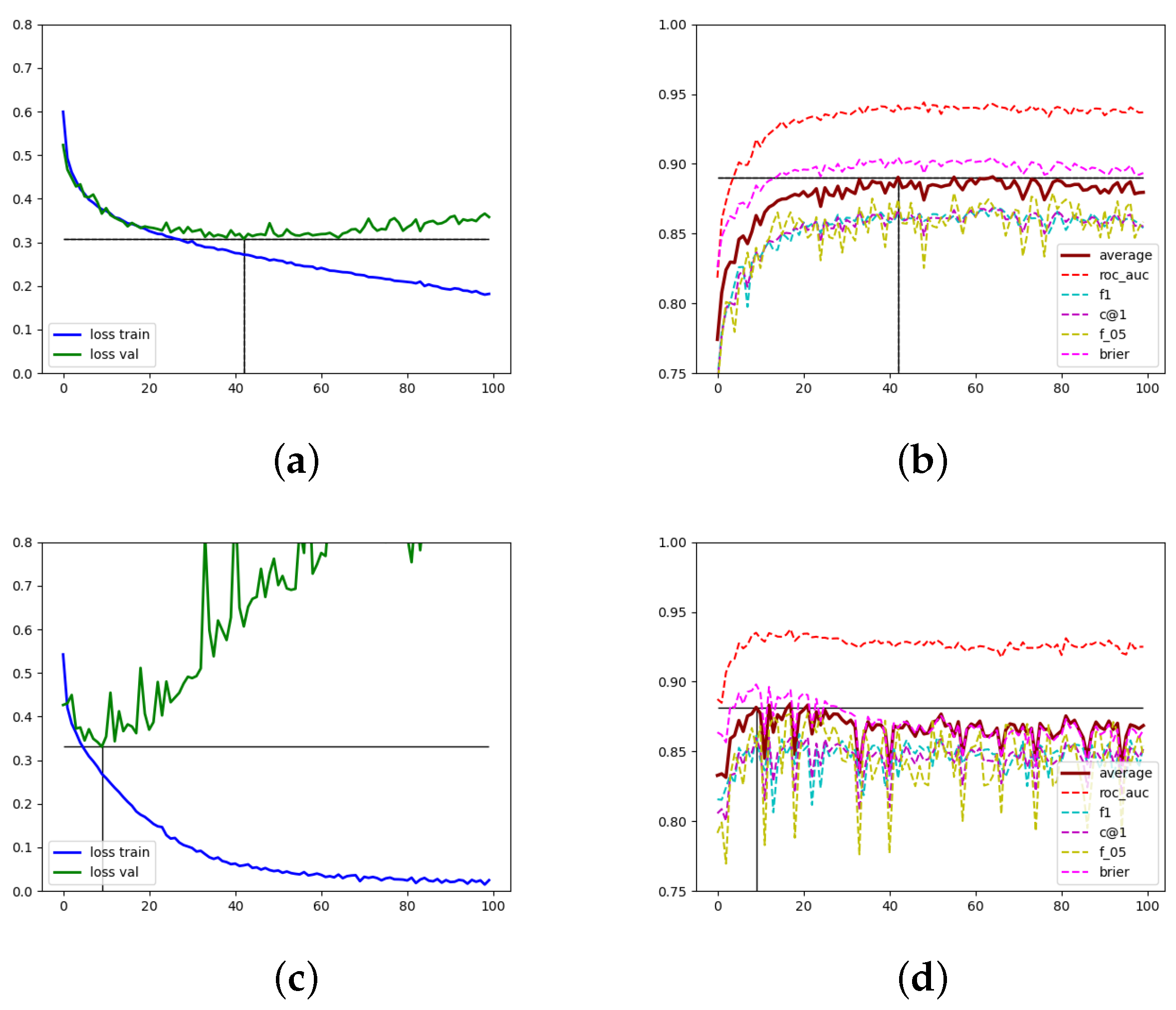
Figure 5 shows how the loss and the five scoring metrics varied along the epochs in training for two executions. The two upper images represent a model with nine layers of LEConv with med graph. The two lower images correspond to a model with three layers of TAGConv with full graph. Figure 5a,c show the loss in training and validation split and Figure 5b,d show the five scores and its average in validation.
Looking carefully at Figure 5a,b we note an inverse correlation between the loss and the scores: when the loss increases the scores decrease and the other way around. We observed these in all the experiments which tells us that our loss objective is a good fit for optimizing our scores. We note that the loss in the validation split is more stable for the model with LEConv layer than for the model with TAGConv layer. The loss and scores for both the GraphConv and GCN2Conv layers have a similar behavior to the model with LEConv. In general, the experiments performed with TAGConv are the most unstable.
4.2.2. Varying the Pooling and Classification Layers
We varied the number of layers used for the global pooling () and the number of layers used in classification (). Table 6 shows the scores for the models using 6 and 9 layers of the LEConv graph convolutional layer and for the models using three layers of the TAGConv graph convolutional layer. Each row shows the number of pooling layers (), the graph representation used and the columns that correspond to the number of classification layers, (). For each architecture tested and graph representation used we highlight with boldface and underline the best results.
- In the experiments over the short graphs, we can notice:
- –
- Using either LEConv or TAGConv layers, the performance is almost always better using four classification layers than using two classification layers. The only exception is in the experiments performed with 9 LEConv layers and .
- –
- The experiments with 6 and 9 LEConv layers compared to those with four classification layers present different behaviors. The performance of the architectures with six LEConv layers decreases when adding more pooling layers and for the architecture with nine layers the performance increases when adding more pooling layers. This may be because the models with nine LEConv layers can learn more complex patterns from the short graph and are improved allowing the attention in the pooling layer to be more expressive. Instead, the models with just 6 LEConv layers overfit when the attention in the pooling layers is too complex.
- –
- When the TAGConv layers are used with two classification layers the performance slightly decreases when we increase the pooling layers. In contrast, when using four classification layers the performance starts growing when we increase the pooling layers.
- With respect to the experiments over the med graphs, we can observe:
- –
- Using TAGConv layers, the performance is better when the architecture uses 4 classification layers than using two classification layers. Furthermore, in these experiments, when the pooling layers increase the performance decreases.
- In the experiments over the full graphs, we can notice:
- –
- When the architecture uses LEConv layers, the models improve their performance with two classification layers instead of 4.
- –
- In particular, when using LEConv layers with two classification layers, the models decrease their performance when adding more than four pooling layers.
- –
- When using TAGConv layers the behavior is different, the best performance is obtained when using four classification layers and four pooling layers; the performance decreases if we vary just one of the parameters, i.e., when we increase the pooling layers to 8 or when we decrease to two classification layers. However, the performance increases again when using both eight pooling layers and two classification layers.
We aim to tune the GBSN and to select the best architecture for the short graph and med graph representations because we will use them as a base of the GBSN Ensemble model in Section 4.3. We did not consider architectures over full graph because the experiments with these graph representations are computationally more expensive and the performance ( in the best architecture) is not much higher than the performance of the architectures over the short graph ( in the best architecture). Table 7 shows the score obtained in individual executions of the best architectures chosen for short graph and med graph. In the first column we show the architecture selected, the second column shows the graph representation, the third column is a number to identify the particular instance, and the last column is the average score of the five evaluation metrics.
4.3. Results of the GBSN Ensemble Architecture
In this section, we show experiments using the GBSN Ensemble architecture. For all our experiments, we fixed the number of classification layers used in the GBSN Ensemble to 5. Given that in the ensemble architecture we concatenate the result of more than one feature extraction component, the input vector of the classification network is larger. We choose to use 5 classification layers to allow the classification network to be more expressive.
From now to the rest of this work, we will refer as Short 1 to the model that corresponds to the first instance of the architecture using the short graph representation from Table 7. Similarly, we will refer with the same nomenclature to the other instances listed in this Table. We made our ensemble experiments using only the best architectures for short and med graphs representations because these are computational less expensive than the architectures using full graph representation.
4.3.1. Results of Different Training Strategies
We evaluated three training strategies:
- To train the GBSN Ensemble architecture all together with random weight initialization.
- First to train the GBSN architecture for each component, second to initialize the weights of the GBSN Ensemble architecture with the weights obtained from the base GBSN architectures, and finally to train the ensemble together without freezing any weights.
- To train the GBSN architecture for each component and to initialize the weights of the GBSN Ensemble as in the previous point and also freeze the weights in the feature extraction components to train only the classification step weights.
Table 8 shows the scores when training GBSN Ensembles. Each row in the table corresponds to an ensemble with the feature extraction components described in the first column. The second column corresponds to the score when training without initialization, the third column corresponds to the score when initializing the weights from the single models but without freezing them, and the last column correspond to the score when initializing the weights and freezing the ones in the feature extraction components. The best performances across different training strategies are highlighted with boldface and underline in each row.
The first row shows the best score obtained by the single GBSN over med graph in a single experiment, as reported before in Table 7. The second row corresponds to an experiment combining two instances of the same feature extraction components over the med graph representation; note that the best individual score was and the best ensemble score was , so using two independent instances let us to increase the performance in more than . The other two rows show models that combine different feature extraction layers. In general, training without transferring the weights showed the worst scores, even lower than the scores achieved when using only single instances (see Table 7). When combining different feature extraction components the best score was obtained when transferring and freezing the weights in the feature extraction components.
Using the last training strategy has another advantage: because of the frozen weights, we just need to train the classification step, so the training is faster. With this strategy, the models achieve the best performance usually in no more than 20 epochs. We will focus the next experiments using this training strategy because the best performance was achieved using this strategy and it also provides less computational cost than the others.
4.3.2. Adding Stylistic Features Component
Until now we evaluated the performance of feature extraction components over graph representations. These graph representations capture mainly the grammatical structure of the texts, so the model may be improved if we include stylistic features. Furthermore, until now, the results reported were obtained training and testing on the “small” dataset splits. In this section, we will show the results of the experiments with the ensemble architectures considering stylistic feature components over the “small” and “large” dataset splits.
Table 9 shows the comparative performance of the evaluated models. Each row shows the average of the five evaluation metrics achieved by a given model when trained and tested on our splits for the “small” and “large” datasets, respectively. We include in this table the performance for the baselines, GBSN with single feature extraction components, and GBSN Ensembles.
The first two rows show the performance of the two selected baselines. The third and fourth rows correspond to the model using only the feature extraction component on the short graph representation and the model using only the feature extraction component on the med graph representation, respectively. The fifth row shows the scores of the model using feature extraction components on both short graph and med graph representation without stylistic features. The sixth row shows the scores of a model with feature components on the short, med graph representations, along with the stylistic features. The seventh row shows the scores of a model combining feature extraction components on two instances of short graph representations and two instances of med graph representations. Finally, the last row shows the scores of a model combining feature extraction components on two short graph representations, two med graph representations, and stylistic features. We highlight with boldface and underline the best results obtained on “small” and “large” dataset splits.
Training on “large” dataset splits improve the performance of all models. Furthermore, all our proposed models considerably outperform the score of the baselines. The inclusion of the stylistic features component allows the architecture to improve the performance when comparing with the equivalent architecture without them. This improvement is more substantial when the models are trained on the “small” dataset splits. When comparing models trained on the “large” dataset splits, adding stylistic features component to the model using one short and med components (Short + Med) just improve and adding stylistic features component to the model using two short and two med components (Short(x2) + Med(x2)) just improve These results indicate that the graph-based models learn better features when more data are available. The GBSN performance when trained on the “large” dataset performed almost as well as when adding the stylistic features.
4.4. Results of the Threshold Adjustment
Our model was initially trained to return an output between 0 and 1. Given a threshold and a margin m we can transform the original output to a new one by following the formula:
This formula linearly transforms the interval into , the interval into and the interval into .
This transformation allows the model to: adjust the best threshold for the binary classification, and predict some difficult problems as ’not answered’, i.e., the model avoids the prediction of verification problems when it is not sure if the text corresponds to the same author or not. The C@1 metric benefits from this behavior because it rewards methods that leave problems unanswered rather than providing wrong answers [42]. As a final tuning, we performed a grid search over different thresholds and margins to optimize the average of the scores in the validation split. Then, we selected the best threshold and margin obtained and evaluate the model in the test split.
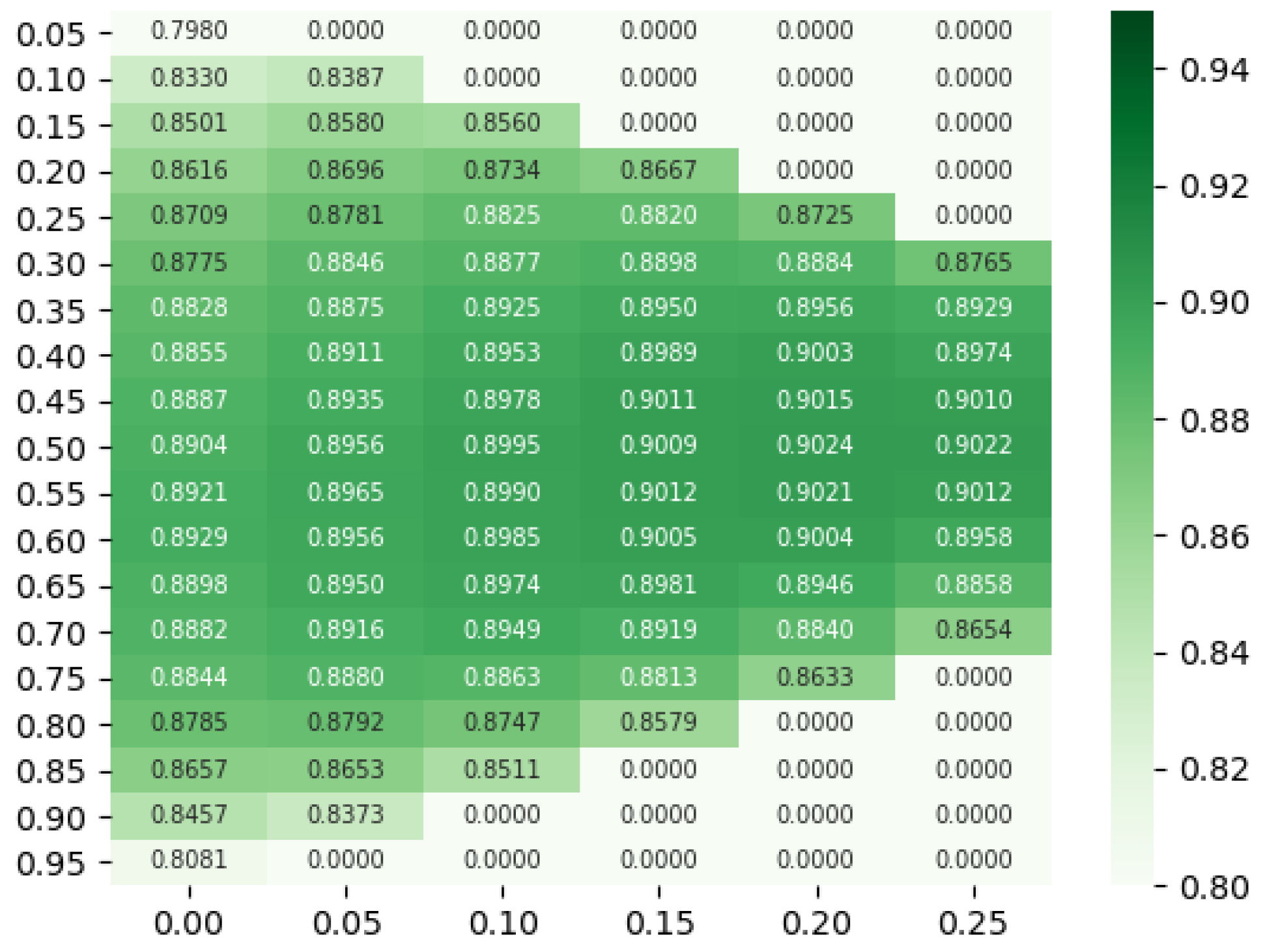
Figure 6 shows a heatmap of the scores when varying the threshold and margin. We searched thresholds values between and and margin values between 0 and , both with increments of . From these results, we can notice that the score increase from in the default threshold-margin of 0.50–0.00 to in the best configuration of 0.50–0.20.
Figure 7a,b shows the distribution for positive and negative instances before and after the threshold adjustment, respectively. The X-axis corresponds to the score obtained by our model and the Y-axis shows the number of problems obtained with these scores. The blue bars are the proportion of problems with a different-author label (0) and the orange bars are the proportion of problems with a same-author label (1).
The different-author labeled problems (blue) are mainly classified with low values and the same-author labeled ones (orange) are mainly classified with high values. With the threshold adjustment, the scores increase mainly because some of the difficult to solve problems were sent to 0.5, i.e., the problems were left unanswered. These unanswered problems are represented in the bar at in Figure 7b.
The threshold adjustment significantly improves the performance of the model in the test split. Table 10 shows the scores and improvements in the “small” and “large” dataset splits for some of our single and ensemble architectures. Each row corresponds to a model presented in Table 9 with the exception of the baselines. The first column shows the name of the model, the second and third are the performance after the threshold adjustment and the improvement when compared with no adjustment in the “small” dataset splits and the fourth and fifth columns are the performance after the threshold adjustment and the improvement when compared with no adjustment in the “large” dataset splits. We highlight with boldface and underline the best results obtained in each dataset split.
4.5. GBSN Performance in the 2021 PAN@CLEF Authorship Verification Shared Task
CLEF 2021 (http://clef2021.clef-initiative.eu/, accessed on 12 January 2022) was the twenty-second edition of the CLEF campaign and workshop series that has run since 2000, it was organized by the University “Politehnica” of Bucharest, Romania, from 21 to 24 September 2021. Their 12 selected labs represented scientific challenges based on new data sets and real-world problems.
One of these labs is PAN: Digital Text Forensics and Stylometry, a networking initiative for digital text forensics (http://pan.webis.de/, accessed on 12 January 2022). PAN provides evaluation resources consisting of large-scale corpora, performance measures, and web services that allow for meaningful evaluations. The PAN 2021 Authorship Verification shared task at adopt the five evaluation metrics used also to evaluate our models: AUC ROC (Area under the ROC Curve), F1 score, Brier score, F0.5u, and C@1. They provided three baseline systems (calibrated on the “small” training set) for comparison:
- A naive distance-based, first-order bag-of-words model [46].
The first two baselines are the same as those presented by us, with the difference that we presented the scores of this baselines trained and tested with exactly the same splits used in all our experiments.
We submit two models to the 2021 PAN@CLEF Authorship Verification task, one trained on the “small” dataset and the other trained on the “large” dataset. Both models have the same architecture: GBSN Ensemble architecture with two short, two med, and stylistic components. Each graph-based component has an architecture of 6 LEConv layers and 4 layers for the fully connected network in the pooling step. The final classification network has 5 layers. The ensemble architecture was trained by transferring and freezing weights from the feature extraction components. Both models are improved with the threshold adjust method proposed in this work.
We obtained the second-best score for the model trained on the “large” dataset and the third-best score for the model trained on the “small” dataset. Table 11 shows the official scores reported in the task overview [33]. The table shows system rankings for PAN 2021 submissions across five evaluation metrics: AUC ROC, c@1, F1, F0.5u, Brier, and an overall mean score (as the final ranking criterion). The dataset column indicates which calibration dataset was used. Our submitted models are marked in bold. The horizontal line indicate the range of scores yielded by the baselines (in italics). We just include the submissions with performance above baselines.
We want to note several relevant points:
- The scores for the GBSN models described in Table 10 are not directly comparable with the scores reported by the PAN task committee. This is because the scores of the first table are obtained testing the models in our test split and the scores of the last table are the ones obtained by PAN in the test dataset, to which we do not have access.
- For our submitted models and the baselines, the scores reported by PAN, measured in the test dataset, were higher than the ones obtained in our test split.
- We do not use any up-sampling technique over the given dataset and, because of our train framework, for each dataset, we train our submitted model using only 90% of the available data; that is, the “small” model was trained using just 47,336 problems and the “large” model using just 247,992 problems; this is relevant because our architecture showed to work better with more training pairs.
The results obtained show us that our proposed approach has performance comparable with the state of the art in this research area. Furthermore, our experiments show us that the approach can improve their performance or be modified to achieve good results with considerably less computational cost.
5. Discussion
In this paper, we presented a novel Siamese network architecture composed of two graph convolutional neural networks with graph level pooling, and classification layers to approach the authorship verification task. For the text representation, we propose three graph models and evaluate their appropriateness for the above-mentioned task. The graph representations from texts are based on the relation of the POS labels and co-occurrence of the words. These representations, allow us to choose which POS labels are masked as a single node in the graph, let us reduce the graph complexity, and focus the representation in POS labels relevant to a specific task.
Specifically, we evaluated the following graph representations: Short, where all words with same POS label are identified to the same node; Med, where POS labels corresponding to adjectives, nouns, adverbs, verbs, cardinal numbers, foreign words, list markers, and symbols are identified as the same node and Full where each tuple of (word, POS) is represented as a node; this corresponds to the traditional co-occurrence graph.
As part of our proposed architecture, we evaluated several graph convolutional layers (LEConv, GraphConv, GCN2Conv, and TAGConv) over the graph representations. We presented detailed scores of our experiments and from them, we can conclude the following:
- Concerning the graph representation used:
- –
- The performance of the architecture (graph convolutional layers, pooling layers, classification layers) are strongly dependent of the graph representation chosen.
- –
- The performance of the models with the med graph is in general better than the performance of the models with short graph and full graph representation. The GBSN model with individual components achieved the best score with the med graph representation.
- –
- The performance of the models with short graph representations show good performance, achieving average scores of 86.64% and 89.47% in the “small” and “large” dataset splits, respectively. Even being a relatively small graph with usually just 33 nodes and 407 edges, this graph is a good alternative to trade off performance for computational cost.
- Concerning the graph convolutional layers used:
- –
- Models with LEConv layer have in general (but not always) better performance than models with GraphConv and GCN2Conv layers over all the graph representations tested. With this kind of layer good performance is obtained when using 6 or 9 layers.
- –
- Models with TAGConv layer have their best performance when using just 3 layers. The scores obtained with these models are the best over full graph representations. Furthermore, the score obtained over the short graph representation (86.59%) is comparable with the best score obtained by the model using LEConv layer over the short graph representation (86.64%).
- –
- When varying the layers used in pooling and the classification layers we cannot conclude a general rule to improve the performance, but our experiments show that both are relevant hyperparameters to consider when tuning a model.
We also proposed combining more than one component for feature extraction, we evaluated graph-based and stylistic-based components with different training strategies. We found that transferring the weights from a single component architecture and freezing these in the ensemble architecture is the best training strategy because it has the best performance and the lowest computational cost.
In general, the combined use of more than one graph-based component improves the performance, even if we use several components based on the same graph representation. Finally, we showed that our architectures can be improved with a simple threshold adjustment, giving us final scores comparable with the state of the art in this task.
The new Graph-based Siamese network showed good performance in the authorship verification task. For future work, we want to evaluate this new approach on other authorship analysis tasks. Furthermore, the proposed graph representation is based on the relation of words, capturing mainly the structural information of the POS labels. Character level information has shown to have good performance in authorship attribution task [13,14], so it will be interesting to generalize the graph representation strategy to include information at the character level.
Author Contributions
Conceptualization, D.E.-R., H.G.-A. and A.E.-R.; Data curation, D.E.-R. and A.E.-R.; Formal analysis, D.E.-R. and H.G.-A.; Funding acquisition, H.G.-A. and G.S.; Investigation, D.E.-R.; Methodology, D.E.-R. and H.G.-A.; Resources, D.E.-R. and H.G.-A.; Software, D.E.-R.; Supervision, H.G.-A. and G.S.; Validation, D.E.-R. and H.G.-A.; Visualization, D.E.-R. and A.E.-R.; Writing—original draft, D.E.-R.; Writing—review & editing, D.E.-R. and H.G.-A. All authors will be informed about each step of manuscript processing including submission, revision, revision reminder, etc. via emails from our system or assigned Assistant Editor. All authors have read and agreed to the published version of the manuscript.
Funding
This research was partially funded by CONACYT PNPC scholarship with No. CVU 1004062, DGAPA-UNAM PAPIIT grant number TA100520, and DGAPA-UNAM PAPIIT grant number IG400119, IT100822.
Data Availability Statement
Restrictions apply to the availability of these data. Data was obtained from PAN (https://pan.webis.de/) and are available at https://0-doi-org.brum.beds.ac.uk/10.5281/zenodo.3716403 and https://0-doi-org.brum.beds.ac.uk/10.5281/zenodo.3724096 with the permission of PAN (https://pan.webis.de/).
Acknowledgments
The authors thank CONACYT for the computer resources provided through the INAOE Supercomputing Laboratory’s Deep Learning Platform for Language Technologies.
Conflicts of Interest
The authors declare no conflict of interest. The funders had no role in the design of the study; in the collection, analyses, or interpretation of data; in the writing of the manuscript, or in the decision to publish the results.
References
- Juola, P. Authorship Attribution. Found. Trends® Inf. Retr. 2007, 1, 233–334. [Google Scholar] [CrossRef]
- Stamatatos, E. A Survey of Modern Authorship Attribution Methods. J. Am. Soc. Inf. Sci. Technol. 2009, 60, 538–556. [Google Scholar] [CrossRef] [Green Version]
- Mekala, S.; Bulusu, V.V. A Survey On Authorship Attribution Approaches. Int. J. Comput. Eng. Res. (IJCER) 2018, 8, 8. [Google Scholar]
- Chaski, C.E. Who’s At The Keyboard? Authorship Attribution in Digital Evidence Investigations. Int. J. Digit. Evid. 2005, 4, 14. [Google Scholar]
- Frantzeskou, G.; Stamatatos, E.; Gritzalis, S.; Katsikas, S. Effective Identification of Source Code Authors Using Byte-Level Information. In Proceedings of the ICSE ’06: Proceedings of the 28th International Conference on Software Engineering, Shanghai, China, 20–28 May 2006; pp. 893–896. [Google Scholar] [CrossRef] [Green Version]
- Stamatatos, E.; Daelemans, W.; Verhoeven, B.; Potthast, M.; Stein, B.; Juola, P.; Sanchez-Perez, M.A.; Barrón-Cedeño, A. Overview of the Author Identification Task at PAN 2014. CLEF 2014, 1180, 877–897. [Google Scholar]
- Koppel, M.; Winter, Y. Determining If Two Documents Are Written by the Same Author. J. Assoc. Inf. Sci. Technol. 2014, 65, 178–187. [Google Scholar] [CrossRef]
- Koppel, M.; Schler, J.; Bonchek-Dokow, E.; Dokow, B. Measuring Differentiability: Unmasking Pseudonymous Authors. J. Mach. Learn. Res. 2007, 8, 1261–1276. [Google Scholar]
- Kestemont, M.; Luyckx, K.; Daelemans, W.; Crombez, T. Cross-Genre Authorship Verification Using Unmasking. Engl. Stud. 2012, 93, 340–356. [Google Scholar] [CrossRef] [Green Version]
- Bevendorff, J.; Stein, B.; Hagen, M.; Potthast, M. Generalizing Unmasking for Short Texts. In Proceedings of the 2019 Conference of the North American Chapter of the Association for Computational Linguistics: Human Language Technologies, Volume 1 (Long and Short Papers), Minneapolis, MN, USA, 2 June 2019; Association for Computational Linguistics: Minneapolis, MN, USA, 2019; pp. 654–659. [Google Scholar] [CrossRef] [Green Version]
- Koppel, M.; Schler, J.; Argamon, S. Authorship Attribution in the Wild. Lang. Resour. Eval. 2011, 45, 83–94. [Google Scholar] [CrossRef]
- Stamatatos, E.; Daelemans, W.; Verhoeven, B.; Juola, P.; López-López, A.; Potthast, M.; Stein, B. Overview of the Author Identification Task at PAN 2015. In Proceedings of the CLEF PAN Conference, Toulouse, France, 8–11 September 2015; p. 17. [Google Scholar]
- Stamatatos, E. On the Robustness of Authorship Attribution Based on Character N-Gram Features. J. Law Policy 2013, 21, 20. [Google Scholar]
- Sapkota, U.; Bethard, S.; Montes, M.; Solorio, T. Not All Character N-Grams Are Created Equal: A Study in Authorship Attribution. In Proceedings of the 2015 Conference of the North American Chapter of the Association for Computational Linguistics: Human Language Technologies, Denver, CO, USA, 31 May–5 June 2015; Association for Computational Linguistics: Denver, CO, USA, 2015; pp. 93–102. [Google Scholar] [CrossRef]
- Petras, V.; Forner, P.; Clough, P.D. (Eds.) Notebook Papers of CLEF 2011 Labs and Workshops, 19–22 September; CEUR-WS: Amsterdam, The Netherlands, 2011. [Google Scholar]
- Bagnall, D. Author Identification Using Multi-Headed Recurrent Neural Networks. arXiv 2015, arXiv:1506.04891. [Google Scholar]
- Jafariakinabad, F.; Tarnpradab, S.; Hua, K.A. Syntactic Recurrent Neural Network for Authorship Attribution. arXiv 2019, arXiv:1902.09723. [Google Scholar]
- Weerasinghe, J.; Greenstadt, R. Feature Vector Difference Based Neural Network and Logistic Regression Models for Authorship Verification. In Notebook for PAN at CLEF 2020; CEUR-WS: Thessaloniki, Greece, 2020; p. 6. [Google Scholar]
- Sonawane, S.S.; Kulkarni, P.A. Graph Based Representation and Analysis of Text Document: A Survey of Techniques. Int. J. Comput. Appl. 2014, 96, 1–8. [Google Scholar] [CrossRef]
- Pinto, D.; Gomez Adorno, H.; Vilariño, D.; Singh, V. A Graph-Based Multi-Level Linguistic Representation for Document Understanding. Pattern Recognit. Lett. 2014, 41, 93–102. [Google Scholar] [CrossRef]
- Castillo, E.; Cervantes, O.; Vilariño, D. Text Analysis Using Different Graph-Based Representations. Comput. Sist. 2017, 21, 581–599. [Google Scholar] [CrossRef]
- Castillo, E.; Cervantes, O.; Vilariño, D. Authorship Verification Using a Graph Knowledge Discovery Approach. J. Intell. Fuzzy Syst. 2019, 36, 6075–6087. [Google Scholar] [CrossRef]
- Gómez-Adorno, H.; Sidorov, G.; Pinto, D.; Vilariño, D.; Gelbukh, A. Automatic Authorship Detection Using Textual Patterns Extracted from Integrated Syntactic Graphs. Sensors 2016, 16, 1374. [Google Scholar] [CrossRef] [Green Version]
- Wu, Z.; Pan, S.; Chen, F.; Long, G.; Zhang, C.; Yu, P.S. A Comprehensive Survey on Graph Neural Networks. IEEE Trans. Neural Netw. Learn. Syst. 2020, 32, 4–24. [Google Scholar] [CrossRef] [PubMed] [Green Version]
- Cruz, L. Authorship Recognition with Short-Text Using Graph-Based Techniques. In Proceedings of the 2019 Workshop on Widening NLP, Florence, Italy, 28 July 2019; Association for Computational Linguistics: Florence, Italy, 2019; pp. 153–156. [Google Scholar]
- Narayanan, A.; Chandramohan, M.; Venkatesan, R.; Chen, L.; Liu, Y.; Jaiswal, S. Graph2vec: Learning Distributed Representations of Graphs. arXiv 2017, arXiv:1707.05005. [Google Scholar]
- Lippincott, T. Graph Convolutional Networks for Exploring Authorship Hypotheses. In Proceedings of the 3rd Joint SIGHUM Workshop on Computational Linguistics for Cultural Heritage, Social Sciences, Humanities and Literature, Minneapolis, MN, USA, 7 June 2019; Association for Computational Linguistics: Minneapolis, MN, USA, 2019; pp. 76–81. [Google Scholar] [CrossRef]
- Bromley, J.; Guyon, I.; LeCun, Y.; Säckinger, E.; Shah, R. Signature Verification Using a “Siamese” Time Delay Neural Network. Int. J. Pattern Recognit. Artif. Intell. 1993, 7, 669–688. [Google Scholar] [CrossRef] [Green Version]
- Nandy, A.; Haldar, S.; Banerjee, S.; Mitra, S. A Survey on Applications of Siamese Neural Networks in Computer Vision. In Proceedings of the 2020 International Conference for Emerging Technology (INCET), Belgaum, India, 5–7 June 2020; pp. 1–5. [Google Scholar] [CrossRef]
- Koch, G.; Zemel, R.; Salakhutdinov, R. Siamese Neural Networks for One-Shot Image Recognition. In Proceedings of the ICML Deep Learning Workshop, Lille, France, 6–11 July 2015; Volume 2, p. 8. [Google Scholar]
- Boenninghoff, B.; Rupp, J.; Nickel, R.M.; Kolossa, D. Deep Bayes Factor Scoring for Authorship Verification. arXiv 2020, arXiv:2008.10105. [Google Scholar]
- Araujo-Pino, E.; Gómez-Adorno, H.; Fuentes-Pineda, G. Siamese Network Applied to Authorship Verification. In Notebook for PAN at CLEF 2020; CEUR: Thessaloniki, Greece, 2020; p. 8. [Google Scholar]
- Kestemont, M.; Manjavacas, E.; Markov, I.; Bevendorff, J.; Wiegmann, M.; Stamatatos, E.; Stein, B.; Potthast, M. Overview of the Cross-Domain Authorship Verification Task at PAN 2021. In Proceedings of the Working Notes of CLEF 2021—Conference and Labs of the Evaluation Forum, Bucharest, Romania, 21–24 September 2021; p. 17. [Google Scholar]
- Marcus, M. Building a Large Annotated Corpus of English: The Penn Treebank; Technical Report; Defense Technical Information Center: Fort Belvoir, VA, USA, 1993. [Google Scholar] [CrossRef]
- Morris, C.; Ritzert, M.; Fey, M.; Hamilton, W.L.; Lenssen, J.E.; Rattan, G.; Grohe, M. Weisfeiler and Leman Go Neural: Higher-Order Graph Neural Networks. In Proceedings of the AAAI Conference on Artificial Intelligence, Honolulu, HI, USA, 27 January–1 February 2019; Volume 33, pp. 4602–4609. [Google Scholar] [CrossRef] [Green Version]
- Ranjan, E.; Sanyal, S.; Talukdar, P.P. ASAP: Adaptive Structure Aware Pooling for Learning Hierarchical Graph Representations. In Proceedings of the Thirty-Fourth AAAI Conference on Artificial Intelligence, New York, NY, USA, 7–12 February 2020. [Google Scholar]
- Kipf, T.N.; Welling, M. Semi-Supervised Classification with Graph Convolutional Networks. arXiv 2016, arXiv:1609.02907. [Google Scholar]
- Chen, M.; Wei, Z.; Huang, Z.; Ding, B.; Li, Y. Simple and Deep Graph Convolutional Networks. In Proceedings of the International Conference on Machine Learning, Vienna, Austria, 12–18 July 2020; PMLR: Vienna, Austria, 2020. [Google Scholar]
- Du, J.; Zhang, S.; Wu, G.; Moura, J.M.F.; Kar, S. Topology Adaptive Graph Convolutional Networks. arXiv 2018, arXiv:1710.10370. [Google Scholar]
- Li, Y.; Tarlow, D.; Brockschmidt, M.; Zemel, R. Gated Graph Sequence Neural Networks. arXiv 2015, arXiv:1511.05493. [Google Scholar]
- Brier, G.W. Verification of Forecasts Expressed in Terms of Probability. Mon. Weather Rev. 1950, 78, 1–3. [Google Scholar] [CrossRef]
- Penas, A.; Rodrigo, A. A Simple Measure to Assess Non-Response. In Proceedings of the 49th Annual Meeting of the Association for Computational Linguistics, Portland, OR, USA, 19–24 June 2011; pp. 1415–1424. [Google Scholar]
- Teahan, W.J.; Harper, D.J. Using Compression-Based Language Models for Text Categorization. In Language Modeling for Information Retrieval; Croft, W.B., Lafferty, J., Eds.; Springer: Dordrecht, The Netherlands, 2003; pp. 141–165. [Google Scholar] [CrossRef]
- Potthast, M.; Braun, S.; Buz, T.; Duffhauss, F.; Friedrich, F.; Gülzow, J.M.; Köhler, J.; Lötzsch, W.; Müller, F.; Müller, M.E.; et al. Who Wrote the Web? Revisiting Influential Author Identification Research Applicable to Information Retrieval. In Lecture Notes in Computer Science; ECIR, Ferro, N., Crestani, F., Moens, M.F., Mothe, J., Silvestri, F., Nunzio, G.M.D., Hauff, C., Silvello, G., Eds.; Springer: Padua, Italy, 2016; Volume 9626, pp. 393–407. [Google Scholar]
- Dehak, N.; Kenny, P.J.; Dehak, R.; Dumouchel, P.; Ouellet, P. Front-End Factor Analysis for Speaker Verification. IEEE Trans. Audio Speech, Lang. Process. 2011, 19, 788–798. [Google Scholar] [CrossRef]
- Kestemont, M.; Stover, J.; Koppel, M.; Karsdorp, F.; Daelemans, W. Authenticating the Writings of Julius Caesar. Expert Syst. Appl. 2016, 63, 86–96. [Google Scholar] [CrossRef] [Green Version]
Figure 1.
(a) Short graph, (b) Med graph, and (c) Full graph.

Figure 2.
GBSN base architecture.

Figure 3.
Global Attention Pooling layer.

Figure 4.
Graph-based Siamese Network Ensemble architecture.

Figure 5.
Loss (a) and scores (b) for GBSN with , , and for med graph. Loss (c) and scores (d) for GBSN with , , and for full graph.
Figure 5.
Loss (a) and scores (b) for GBSN with , , and for med graph. Loss (c) and scores (d) for GBSN with , , and for full graph.

Figure 6.
Threshold grid search in val split for GBSN with parameters LEConv, , , over med graph. As reference the average score without adjust is .
Figure 6.
Threshold grid search in val split for GBSN with parameters LEConv, , , over med graph. As reference the average score without adjust is .

Figure 7.
Histogram of distribution for positive and negative instances: (a) Before threshold adjust (b) With threshold adjust of and .
Figure 7.
Histogram of distribution for positive and negative instances: (a) Before threshold adjust (b) With threshold adjust of and .


Table 1.
Number of problems, texts, authors and topics in the “small” and “large” datasets.
| Problems | Texts | Authors | Topics | |
|---|---|---|---|---|
| “Small” | 52,601 | 93,662 | 52,654 | 1600 |
| “Large” | 275,565 | 494,226 | 278,162 | 1600 |
Table 2.
Total and positive problems for each split.
| “Small” Dataset | “Large” Dataset | |||
|---|---|---|---|---|
| Total | Positive | Total | Positive | |
| Train split | 42,077 | 22,560 | 220,438 | 120,201 |
| Val split | 5259 | 2636 | 27,554 | 13,783 |
| Test split | 5259 | 2633 | 27,554 | 13,777 |
Table 3.
Average nodes and edge number for each graph construction in “large” dataset for the PAN 2021 Authorship Verification task.
Table 3.
Average nodes and edge number for each graph construction in “large” dataset for the PAN 2021 Authorship Verification task.
| Short | Med | Full | |
|---|---|---|---|
| Nodes | 33 | 138 | 1207 |
| Edges | 407 | 1168 | 3424 |
Table 4.
Results obtained by the baseline methods on our train and test splits of the “small” and “large” datasets.
Table 4.
Results obtained by the baseline methods on our train and test splits of the “small” and “large” datasets.
| Baseline | Test Split | AUC | F1 | c@1 | F_0.5u | Brier | Overall |
|---|---|---|---|---|---|---|---|
| Compression | “Small” | 77.40 | 70.60 | 68.70 | 68.20 | 80.30 | 73.00 |
| “Large” | 77.50 | 72.10 | 69.40 | 68.50 | 80.10 | 73.50 | |
| Cosine | “Small” | 76.00 | 75.60 | 69.60 | 67.20 | 78.10 | 73.30 |
| “Large” | 77.60 | 78.80 | 69.50 | 67.20 | 78.30 | 74.30 |
Table 5.
Varying L and . NR = Not reported due to computational cost, ** = Score of only one execution.
Table 5.
Varying L and . NR = Not reported due to computational cost, ** = Score of only one execution.
| Type | Graph | ||||
|---|---|---|---|---|---|
| Short | 85.67 | 86.64 | 85.93 | 86.25 | |
| LEConv | Med | 86.39 | 86.69 | 87.18 | 87.19 |
| Full | 85.75 | 86.01 | 85.94 | NR | |
| Short | 85.72 | 85.95 | 86.29 | 86.05 | |
| GraphConv | Med | 85.97 | 86.50 | 86.94 | 86.45 |
| Full | 84.95 | 86.03 | 86.53 | NR | |
| Short | 85.33 | 86.19 | 85.81 | 86.37 | |
| GCN2Conv | Med | 85.46 | 86.50 | 85.72 | 85.85 |
| Full | 83.79 | 84.98 | 84.68 | NR | |
| Short | 86.34 | 83.65 | 82.19 | 80.76 | |
| TAGConv | Med | 86.02 | 83.22 | 80.22 | 80.45 |
| Full | 86.82 | 84.92 | 83.00 ** | NR |
Table 6.
Experiments when varying , and L. NR = Not reported due to computational cost.
| TAGConv, | LEConv, | LEConv, | |||||
|---|---|---|---|---|---|---|---|
| Graph | 2 | 4 | 2 | 4 | 2 | 4 | |
| Short | 86.06 | 86.34 | 86.08 | 86.64 | 85.72 | 85.93 | |
| 4 | Med | 85.52 | 86.02 | 86.60 | 86.69 | 86.85 | 87.18 |
| Full | 86.50 | 86.82 | 86.84 | 86.01 | 86.62 | 85.94 | |
| Short | 85.95 | 86.38 | 85.62 | 86.22 | 86.22 | 86.08 | |
| 6 | Med | 85.18 | 85.85 | 86.91 | 86.72 | 86.51 | 86.82 |
| Full | 85.92 | 86.80 | 86.81 | 86.37 | 86.43 | 86.11 | |
| Short | 85.85 | 86.59 | 86.03 | 86.08 | 85.57 | 86.60 | |
| 8 | Med | 85.16 | 85.82 | 85.96 | 86.66 | 86.90 | 87.45 |
| Full | 86.65 | 85.88 | 86.06 | 85.81 | NR | NR | |
Table 7.
Best instances of the architectures selected for short graph and med graph.
| Architecture | Graph | Instance | Score | |||
|---|---|---|---|---|---|---|
| LEConv | 6 | 4 | 4 | Short | 1 | 86.73 |
| 2 | 86.65 | |||||
| LEConv | 9 | 8 | 4 | Med | 1 | 87.50 |
| 2 | 87.43 | |||||
Table 8.
GBSN Ensemble with different training strategies. N/A = It is not possible to train the model with this strategy.
Table 8.
GBSN Ensemble with different training strategies. N/A = It is not possible to train the model with this strategy.
| No Transfer | Transfer Weights | ||
|---|---|---|---|
| No Freezing | Freezing | ||
| Med 1 (reference) | 87.50 | N/A | N/A |
| Med 1 + Med 2 | 86.80 | 88.51 | 88.30 |
| Short 1 + Med 1 | 86.59 | 88.53 | 88.64 |
| Short 1 + Short 2 + Med 1 + Med 2 | 86.66 | 88.34 | 88.85 |
Table 9.
Average performance of Graph-based Siamese Network (GBSN) with single and ensemble feature extraction components. Ensemble was training transferring and freezing feature extraction components weights. ** = Score of only one execution.
Table 9.
Average performance of Graph-based Siamese Network (GBSN) with single and ensemble feature extraction components. Ensemble was training transferring and freezing feature extraction components weights. ** = Score of only one execution.
| Model | “Small” Dataset Splits | “Large” Dataset Splits |
|---|---|---|
| Baseline compression | 73.00 ** | 73.50 ** |
| Baseline cosine | 72.90 ** | 74.30 ** |
| Short | 86.64 | 89.47 |
| Med | 87.45 | 90.35 |
| Short + Med | 88.64 | 91.35 |
| Short + Med + Stylistic features | 89.13 | 91.36 |
| Short(x2) + Med(x2) | 88.85 | 91.66 |
| Short(x2) + Med(x2) + Stylistic features | 89.31 | 91.68 |
Table 10.
Average performance after threshold and margin adjust of Graph-based Siamese Network (GBSN) with single and ensemble feature extraction components. Ensemble was trained transferring and freezing feature extraction component weights.
Table 10.
Average performance after threshold and margin adjust of Graph-based Siamese Network (GBSN) with single and ensemble feature extraction components. Ensemble was trained transferring and freezing feature extraction component weights.
| “Small” Dataset | “Large” Dataset | |||
|---|---|---|---|---|
| After Adjustment | Increment | After Adjustment | Increment | |
| Short | 87.87 | 1.23 | 90.63 | 1.16 |
| Med | 88.59 | 1.14 | 91.53 | 1.18 |
| Short + Med | 89.70 | 1.06 | 92.45 | 1.10 |
| Short + Med + Stylistic features | 90.30 | 1.17 | 92.45 | 1.09 |
| Short(x2) + Med(x2) | 89.86 | 1.01 | 92.80 | 1.14 |
| Short(x2) + Med(x2) + Stylistic features | 90.56 | 1.25 | 92.83 | 1.15 |
Table 11.
System rankings for all PAN 2021 submissions. Taken from [33].
Table 11.
System rankings for all PAN 2021 submissions. Taken from [33].
| Team | Dataset | AUC | c@1 | F1 | F0.5u | Brier | Overall |
|---|---|---|---|---|---|---|---|
| boenninghoff21 | “large” | 0.9869 | 0.9502 | 0.9524 | 0.9378 | 0.9452 | 0.9545 |
| embarcaderoruiz21 | “large” | 0.9697 | 0.9306 | 0.9342 | 0.9147 | 0.9305 | 0.9359 |
| weerasinghe21 | “large” | 0.9719 | 0.9172 | 0.9159 | 0.9245 | 0.9340 | 0.9327 |
| weerasinghe21 | “small” | 0.9666 | 0.9103 | 0.9071 | 0.9270 | 0.9290 | 0.9280 |
| menta21 | “large” | 0.9635 | 0.9024 | 0.8990 | 0.9186 | 0.9155 | 0.9198 |
| peng21 | “small” | 0.9172 | 0.9172 | 0.9167 | 0.9200 | 0.9172 | 0.9177 |
| embarcaderoruiz21 | “small” | 0.9470 | 0.8982 | 0.9040 | 0.8785 | 0.9072 | 0.9170 |
| menta21 | “small” | 0.9385 | 0.8662 | 0.8620 | 0.8787 | 0.8762 | 0.8843 |
| rabinovits21 | “small” | 0.8129 | 0.9129 | 0.8094 | 0.8186 | 0.8129 | 0.8133 |
| ikae21 | “small” | 0.9041 | 0.7586 | 0.8145 | 0.7233 | 0.8247 | 0.8050 |
| unmasking21 | “small” | 0.8298 | 0.7707 | 0.7803 | 0.7466 | 0.7904 | 0.7836 |
| tyo21 | “large” | 0.8275 | 0.7594 | 0.7911 | 0.7257 | 0.8123 | 0.7832 |
| naive21 | “small” | 0.7956 | 0.7320 | 0.7856 | 0.6998 | 0.7867 | 0.7600 |
| compressor21 | “small” | 0.7896 | 0.7282 | 0.7609 | 0.7027 | 0.8094 | 0.7581 |
Publisher’s Note: MDPI stays neutral with regard to jurisdictional claims in published maps and institutional affiliations. |
© 2022 by the authors. Licensee MDPI, Basel, Switzerland. This article is an open access article distributed under the terms and conditions of the Creative Commons Attribution (CC BY) license (https://creativecommons.org/licenses/by/4.0/).
Share and Cite
MDPI and ACS Style
Embarcadero-Ruiz, D.; Gómez-Adorno, H.; Embarcadero-Ruiz, A.; Sierra, G. Graph-Based Siamese Network for Authorship Verification. Mathematics 2022, 10, 277. https://0-doi-org.brum.beds.ac.uk/10.3390/math10020277
AMA Style
Embarcadero-Ruiz D, Gómez-Adorno H, Embarcadero-Ruiz A, Sierra G. Graph-Based Siamese Network for Authorship Verification. Mathematics. 2022; 10(2):277. https://0-doi-org.brum.beds.ac.uk/10.3390/math10020277
Chicago/Turabian StyleEmbarcadero-Ruiz, Daniel, Helena Gómez-Adorno, Alberto Embarcadero-Ruiz, and Gerardo Sierra. 2022. "Graph-Based Siamese Network for Authorship Verification" Mathematics 10, no. 2: 277. https://0-doi-org.brum.beds.ac.uk/10.3390/math10020277
Note that from the first issue of 2016, this journal uses article numbers instead of page numbers. See further details here.