Impulsive Control of Complex-Valued Neural Networks with Mixed Time Delays and Uncertainties

Abstract

This paper investigates the global exponential stability of uncertain delayed complex-valued neural networks (CVNNs) under an impulsive controller. Both discrete and distributed time-varying delays are considered, which makes our model more general than previous works. Unlike most existing research methods of decomposing CVNNs into real and imaginary parts, some stability criteria in terms of complex-valued linear matrix inequalities (LMIs) are obtained by employing the complex Lyapunov function method, which is valid regardless of whether the activation functions can be decomposed. Moreover, a new impulsive differential inequality is applied to resolve the difficulties caused by the mixed time delays and delayed impulse effects. Finally, an illustrative example is provided to back up our theoretical results.

1. Introduction

In recent decades, neural network models have a lot of potential to be used in various fields such as pattern classification, optoelectronics, associative memory and signal processing [1,2,3,4,5]. As the applications of neural networks with complex-valued inputs successfully spread, the stability analysis of CVNNs is a growing research area. Compared with real-valued systems, CVNNs have more complex characteristics which are not only able to simulate much more practical situations but are also able to deal with problems that real-valued systems cannot solve. For example, many applications of associative memories, including the retrieval of gray-scale images in the presence of noise, require the storage of multistate or complex-valued patterns. Another example is the XOR problem and the detection of symmetry problem, which can be solved by a single complex-valued neuron under the orthogonal decision boundaries, but not with their real-valued counterparts. This reveals the strengthened potent computational power of complex-valued neurons. For more engineering applications, we refer the reader to [6,7,8,9,10] and the references therein. Moreover, since the inherent neuron communication and the switching speed of amplifiers are finite, there are inevitably time delays in neural networks, which may cause undesirable performances and even system instability [11,12,13,14]. Therefore, the study of CVNNs with time delays has drawn significant scholarly attention [15,16,17,18,19,20,21,22].

In real-valued neural networks, their activation functions are usually chosen to be smooth and bounded. However, in the complex domain, based on Liouville’s theorem [23], every bounded entire function must be constant. Therefore, activation functions are the main challenge for CVNNs [15]. According to different types of activation functions, the research methods for the stability of CVNNs can be classified into two types. The first method is to separate it into real and imaginary parts to form an equivalent real-valued systems [15,16,17,18]. For example, in [15], the global stability of CVNNs with constant delays was investigated when activation functions were denoted as $f\left(z\right)=f^R(x,y)+i{f}^I(x,y)$. In [16], the authors obtained some criteria for boundedness and the complete stability of CVNNs with time delays. One can observe that this method requires the activation functions to be explicitly decomposed into their real and imaginary parts. However, this separation cannot always be expressed in an analytical form. To solve this problem, a complex-valued Lyapunov function method was proposed as another efficient way of handling CVNNs [19,20,21,22]. Fang and Sun [19] addressed the stabilization of complex-valued recurrent neural networks with time delays through constructing appropriate complex-valued Lyapunov functions. In [21,22], the stability problem of CVNNs with impulsive effect and mixed time delays is concerned via the complex Lyapunov functions method.

As we know, for control problems of neural networks, various approaches, such as pinning control, sampled data control, adaptive control, impulsive control and intermittent state feedback control have been proposed [24,25,26,27,28]. The impulsive control, as a hybrid control approach, has attracted significant interest in many applications [29,30,31,32], since its control input is only imposed on the topological structure of systems at some discrete moments, which can dramatically decrease the quantity of transmitted information and control cost. Hence, a great many attractive results on the impulsive control of delayed neural networks have been presented in recent years [33,34,35,36]. However, there has been limited work on delayed complex-valued systems [37,38,39,40]. In [37], the exponential stabilization of complex-valued inertial neural networks with time-varying delays was analyzed by utilizing impulsive control. Refs. [38,39] presented the synchronization of delayed CVNNs, in which impulsive controllers were used to achieve master–slave exponential synchronization. Most recently, the impulsive control problem of CVNNs with constant delays was studied in [40] by employing the Lyapunov–Razumikhin technique in complex domains.

Note that most results mentioned above are working on the system whose parameters are known and time delays are only of discrete nature. However, in reality, the exact values of parameters are very hard to acquire in neural networks because of modeling inaccuracies or external disturbances. Meanwhile, neural networks always have spatial characteristics because there are plenty of parallel paths with several axon sizes, which means that the signal transmission is not usually instantaneous. Introducing distributed delays to simulate them is very essential. In addition, since it takes a certain amount of time to receive and transmit signals from the controller to the controlled system, including a time delay in the impulsive control input makes more sense. However, to the best of our knowledge, few studies have focused on the stabilization of CVNNs with both discrete and distributed time-varying delays as well as uncertain parameters via delayed impulsive control. This is the motivation of the present paper.

This study deals with the exponential stability of uncertain CVNNs with both discrete and distributed time-varying delays by time-delay impulsive control. The major contributions can be listed as follows: (i) a comprehensive model of CVNNs which simultaneously contains uncertain parameters and mixed time-delays is discussed; (ii) by constructing complex-valued Lyapunov function and designing a delayed impulsive controller, some stability criteria are derived for CVNNs, which are valid regardless of whether the activation functions can be decomposed. Our results extend those of previous studies [37,40]; and (iii) a new impulsive differential inequality is employed to resolve the difficulties caused by the delayed impulse effects and mixed delays. The structure of this study is as follows. Section 2 introduces the models and knowledge related to CVNNs. In Section 3, the main stability results are obtained. An explicit example is presented in Section 4. Section 5 makes a summary of the paper.

Notation 1.

Throughout this paper, let ${\mathbb{C}}^n$ and ${\mathbb{C}}^{n\times n}$ be the set of n-dimensional complex-valued spaces and $n\times n$ complex-valued matrices, respectively. ${\mathbb{R}}^{n\times n}$ denotes $n\times n$ real-valued matrices. Let ${\mathbb{Z}}_{+}$ define the set of positive integers. For a Hermitian matrix P, ${\lambda }_{min}\left(P\right)$ and ${\lambda }_{max}\left(P\right)$ mean the minimum and maximum eigenvalues of matrix P. $\tau \vee \beta$ represents the maximum values of τ and β, $\Lambda =\{1,2,\cdots ,n\}.$ $A<0$ represents that the matrix A is a negative definite matrix. $A\le 0$ or $A\ge 0$ means that the matrix A is a symmetric negative semi-definite or positive semi-definite matrix. Moreover, $A^{-1}$ represents the inverse of A. The notation $\parallel A\parallel$ means the spectral norm of matrix A. For complex-valued vector $\check{z}\in {\mathbb{C}}^n$, $\parallel \check{z}\parallel =\sqrt{\check{z}{\check{z}}^{*}}$, where ${\check{z}}^{*}$ is the conjugate transpose of $\check{z}$. $\parallel \check{z}{\parallel }_{\varrho }=\underset{s\in [-\varrho ,0]}{sup}\parallel \check{z}\left(s\right)\parallel$. $\mathcal{PC}(J,V)=\{\vartheta :J\to V$ denotes continuous everywhere except at a finite number of points t, at which $\vartheta \left(t^{+}\right),$ $\vartheta \left(t^{-}\right)$ exist and $\vartheta \left(t^{+}\right)=\vartheta \left(t\right)\}$. Notation I means that the identity matrix with appropriate dimensions and 🟉 always denotes the symmetric block in one symmetric matrix.

2. Preliminaries

This section studies CVNNs with uncertain parameters and mixed delays as follows:

$$\begin{array}{c}\hfill \left\{\begin{array}{c}\dot{x}\left(t\right)=-C\left(t\right)x\left(t\right)+A\left(t\right)f\left(x\left(t\right)\right)+B\left(t\right)f\left(x(t-\tau \left(t\right))\right)+D\left(t\right){\int }_{t-\beta \left(t\right)}^{t}f\left(x\left(s\right)\right)ds+J, t>0,\hfill \\ x\left(t\right)=\vartheta \left(t\right), t\in [-{\varrho }_1,0],\hfill \end{array}\right.\end{array}$$

(1)

where $x\left(t\right)={(x_1\left(t\right),x_2\left(t\right),\cdots ,x_n\left(t\right))}^T\in {\mathbb{C}}^n$ denotes the state vector of the system, $f\left(x\left(t\right)\right)={(f_1\left(x_1\left(t\right)\right),f_2\left(x_2\left(t\right)\right),\dots ,f_n\left(x_n\left(t\right)\right))}^T\in {\mathbb{C}}^n$ is the neuron activation function; $C\left(t\right)=C+\Delta C\left(t\right)$, $A\left(t\right)=A+\Delta A\left(t\right)$, $B\left(t\right)=B+\Delta B\left(t\right)$, $D\left(t\right)=D+\Delta D\left(t\right)$, in which $C\in {\mathbb{R}}^{n\times n}$ is a positive diagonal matrix, $A\in {\mathbb{C}}^{n\times n}$, $B\in {\mathbb{C}}^{n\times n}$, $D\in {\mathbb{C}}^{n\times n}$ are the connection weight matrices, $\Delta C\left(t\right),$ $\Delta A\left(t\right),$ $\Delta B\left(t\right),$ $\Delta D\left(t\right)$ are time-varying parametric uncertainties; J is the external input of the CVNNs; $\tau \left(t\right)$ and $\beta \left(t\right)$ are the transmission delays and distributed delays, respectively, which satisfy $0\le \tau \left(t\right)\le \tau$, $0\le \beta \left(t\right)\le \beta$, where $\tau$ and $\beta$ are constants; $\vartheta (·)\in \mathcal{PC}([-{\varrho }_1,0],{\mathbb{C}}^n)$ is the initial condition, where ${\varrho }_1=\tau \vee \beta$.

For further discussion, the following assumptions are made:

$\left(H_1\right)$ There exists a positive diagonal matrix $L=diag(L_1,L_2,\dots ,L_n)$ such that:

$$\begin{array}{c}\hfill \Vert f_i\left({\check{u}}_1\right)-f_i\left({\check{u}}_2\right)\Vert \le L_i\Vert {\check{u}}_1-{\check{u}}_2\Vert , i\in \Lambda ,\end{array}$$

for all ${\check{u}}_1,$ ${\check{u}}_2\in \mathbb{C}$.

$\left(H_2\right)$ The time-varying parametric uncertainties $\Delta A\left(t\right),$ $\Delta B\left(t\right),$ $\Delta C\left(t\right),$ $\Delta D\left(t\right)$ are supposed to be of the form:

$$\begin{array}{c}\hfill \left(\Delta C\left(t\right),\Delta A\left(t\right),\Delta B\left(t\right),\Delta D\left(t\right)\right)=TK\left(t\right)({\widehat{U}}_1,{\widehat{U}}_2,{\widehat{U}}_3,{\widehat{U}}_4),\end{array}$$

where T, ${\widehat{U}}_1$, ${\widehat{U}}_2$, ${\widehat{U}}_3$, ${\widehat{U}}_4$ are known matrices, and $K\left(t\right)$ is the matrix of appropriate dimensions satisfying $K^{*}\left(t\right)K\left(t\right)\le I$.

Assume that $\check{x}={({\check{x}}_1,{\check{x}}_2,\cdots ,{\check{x}}_n)}^T$ is an equilibrium point of system (1). Let $\check{z}=x-\check{x}$. Then, the equilibrium point $\check{x}$ is converted to zero. To achieve the stability of CVNNs, the following impulsive control law is designed:

$$\begin{array}{c}\hfill \left\{\begin{array}{c}0\le t_0<t_1<\cdots <t_k\to \infty , k\to \infty ,\hfill \\ \Delta \check{z}\left(t\right)=E_k\check{z}\left(t^{-}\right)+F_k\check{z}(t^{-}-\eta \left(t^{-}\right)), t=t_k,\hfill \end{array}\right.\end{array}$$

(2)

where $E_k,$ $F_k\in {\mathbb{C}}^{n\times n}$ denote impulsive gain matrices at impulsive time $t_k$; $\Delta \check{z}\left(t\right)=\check{z}\left(t\right)-\check{z}\left(t^{-}\right)$; $\eta \left(t\right)$ denotes a time-varying delay and satisfies $0\le \eta \left(t\right)\le \eta$. Let $\mathcal{A}=\left\{t_k\right\}$ be an impulsive sequence satisfying the first inequality of (2), and ${\mathcal{A}}_{\asymp }$ be a subset of $\mathcal{A}$ satisfying $t_k-t_{k-1}\le \zeta$ for any $k\in {\mathbb{Z}}_{+}$, where $\zeta$ is a positive constant.

The system (1) can be converted into the following form:

$$\begin{array}{c}\hfill \left\{\begin{array}{c}\dot{\check{z}}\left(t\right)=-C\left(t\right)\check{z}\left(t\right)+A\left(t\right)F\left(\check{z}\left(t\right)\right)+B\left(t\right)F\left(\check{z}(t-\tau \left(t\right))\right)+D\left(t\right){\int }_{t-\beta \left(t\right)}^{t}F\left(\check{z}\left(s\right)\right)ds, t\ne t_k,\hfill \\ \Delta \check{z}\left(t\right)=E_k\check{z}\left(t^{-}\right)+F_k\check{z}(t^{-}-\eta \left(t^{-}\right)), t=t_k,\hfill \\ \check{z}\left(t\right)=\chi \left(t\right), \forall t\in [-\varrho ,0],\hfill \end{array}\right.\end{array}$$

(3)

where $\chi (·)=\vartheta (·)-\check{x}$, $\chi (·)\in \mathcal{PC}([-\varrho ,0],{\mathbb{C}}^n)$, $F\left(\check{z}\right)=f(\check{z}+\check{x})-f\left(\check{x}\right)$, $\varrho =\tau \vee \beta \vee \eta$.

Definition 1.

In ([41]) The zero equilibrium point of system (3) is said to be globally exponentially stable over the impulse set ${\mathcal{A}}_{\asymp }$, if for any solution of (3), there exist constants $\lambda >0$ and $W>1$ such that $\parallel \check{z}\left(t\right)\parallel \le W{\parallel \chi \parallel }_{\varrho }{e}^{-\lambda t}$, for all $t\ge 0$.

Lemma 1.

In ([42]) Considering the following impulsive differential inequality:

$$\begin{array}{c}\hfill \left\{\begin{array}{c}{D}^{+}V\left(t\right)\le aV\left(t\right)+b\overline{V}\left(t\right), t\ne t_k,\hfill \\ V\left(t\right)\le {\delta }_{1}V\left(t^{-}\right)+{\delta }_2\overline{V}\left(t^{-}\right), t=t_k, k\in {\mathbb{Z}}_{+},\hfill \end{array}\right.\end{array}$$

(4)

where $\overline{V}\left(t\right)=\underset{s\in [t-\varrho ,t]}{sup}V\left(s\right)$. If there exist constants $a\in \mathbb{R},$ $b>0$, ${\delta }_1,$ ${\delta }_2>0$ such that:

$$\begin{array}{c}\hfill {\delta }_1+{\delta }_2<1,\hspace{1em}a+\frac{b}{{\delta }_1+{\delta }_2}<\frac{ln\frac{1}{{\delta }_1+{\delta }_2}}{\zeta },\end{array}$$

then the solution of inequality (4) satisfies:

$$\begin{array}{c}\hfill V\left(t\right)\le \overline{V}\left(0\right)\alpha e^{-\lambda t}, t\ge 0\end{array}$$

over the class ${\mathcal{A}}_{\asymp }$, where α and λ are positive constants with $\alpha >1$ and $\lambda >0$.

Lemma 2.

In ([21]) For any positive definite Hermitian matrix $E\in {\mathbb{C}}^{n\times n}$, a vector function $\upsilon :[c,d]\to {\mathbb{C}}^n$ with scalars $c<d$ such that the related integration is well defined, it follows that:

$$\begin{array}{c}\hfill {\left({\int }_c^d\upsilon \left(s\right)ds\right)}^{*}E{\int }_c^d\upsilon \left(s\right)ds\le (d-c){\int }_c^d{\upsilon }^{*}\left(s\right)E\upsilon \left(s\right)ds.\end{array}$$

Lemma 3.

In ([21]) For any positive Hermitian matrix $R\in {\mathbb{C}}^{n\times n}$, vectors $x,$ $z\in {\mathbb{C}}^n$, it follows that:

$$\begin{array}{c}\hfill x^{*}z+z^{*}x\le x^{*}Rx+z^{*}{R}^{-1}z.\end{array}$$

Lemma 4.

In ([43]) If $\Gamma ,$ Ω and Υ are complex-valued matrices of appropriate dimensions and ${{\rm Y}}^{*}={\rm Y}$, then:

$$\begin{array}{c}\hfill {\rm Y}+\Gamma S\left(t\right)\Omega +{\Omega }^{*}{S}^{*}\left(t\right){\Gamma }^{*}<0\end{array}$$

holds, for all matrices $S\left(t\right)$ satisfying $S^{*}\left(t\right)S\left(t\right)\le I$, if and only if there exists a constant $\epsilon >0$, such that:

$$\begin{array}{c}\hfill {\rm Y}+\epsilon \Gamma {\Gamma }^{*}+{\epsilon }^{-1}{\Omega }^{*}\Omega <0\end{array}$$

holds.

3. Main Results

In this section, some criteria for the globally exponentially stable of the CVNNs (3) are derived based on a complex-valued Lyapunov function and the impulsive differential inequality technique.

Theorem 1.

Suppose that $\left(H_1\right)$ holds. If there exist some constants $a\in \mathbb{R},$ $b>0,$ $\zeta >0,$ ${\delta }_1>0,$ ${\delta }_2>0({\delta }_1+{\delta }_2<1),$ $0<\mu <1$ and a positive definite Hermitian matrix P, positive definite diagonal matrices $G,$ $Q,$ $M\in {\mathbb{R}}^{n\times n}$ such that following inequalities hold:

$$\begin{array}{c}\hfill {\Xi }_1=\left[\begin{array}{cccc}{\acute{\Xi }}_{11}& {\acute{\Xi }}_{12}& {\acute{\Xi }}_{13}& {\acute{\Xi }}_{14}\\ 🟉& -G& 0& 0\\ 🟉& 🟉& -Q& 0\\ 🟉& 🟉& 🟉& -M\end{array}\right]<0,\end{array}$$

(5)

$$\begin{array}{c}\hfill {\Pi }_1=\left[\begin{array}{ccc}-P& P{E}_k+P& P{F}_k\\ 🟉& -{\delta }_{1}P& 0\\ 🟉& 🟉& -{\delta }_{2}P\end{array}\right]\le 0,\end{array}$$

(6)

$$\begin{array}{c}\hfill \left\{\begin{array}{c}\mu bP-LQL\ge 0,\hfill \\ (1-\mu )bP-{\beta }^{2}LML\ge 0,\hfill \end{array}\right.\end{array}$$

(7)

$$\begin{array}{c}\hfill a+\frac{b}{{\delta }_1+{\delta }_2}+\frac{ln({\delta }_1+{\delta }_2)}{\zeta }<0,\end{array}$$

(8)

with:

${\acute{\Xi }}_{11}=-PC\left(t\right)-C^{*}\left(t\right)P+LGL-aP$, ${\acute{\Xi }}_{12}=PA\left(t\right)$, ${\acute{\Xi }}_{13}=PB\left(t\right)$, ${\acute{\Xi }}_{14}=PD\left(t\right)$,then the CVNNs (3) are globally exponentially stable over the set ${\mathcal{A}}_{\asymp }$.

Proof. 

Consider the Lyapunov function:

$$\begin{array}{c}\hfill V\left(t\right)={\check{z}}^{*}\left(t\right)P\check{z}\left(t\right).\end{array}$$

(9)

Taking the derivative of $V\left(t\right)$ along the trajectory of CVNNs (3), one has, for $t\in [t_{k-1},t_k)$, $k\in {\mathbb{Z}}_{+}$:

$$\begin{array}{cc}\hfill D^{+}V\left(t\right)=& {\check{z}}^{*}\left(t\right)P\dot{\check{z}}\left(t\right)+{\dot{\check{z}}}^{*}\left(t\right)P\check{z}\left(t\right)\hfill \\ \hfill =& {\check{z}}^{*}\left(t\right)P[-C\left(t\right)\check{z}\left(t\right)+A\left(t\right)F\left(\check{z}\left(t\right)\right)+B\left(t\right)F\left(\check{z}(t-\tau \left(t\right))\right)+D\left(t\right){\int }_{t-\beta \left(t\right)}^{t}F\left(\check{z}\left(s\right)\right)ds]\hfill \\ & +{[-C\left(t\right)\check{z}\left(t\right)+A\left(t\right)F\left(\check{z}\left(t\right)\right)+B\left(t\right)F\left(\check{z}(t-\tau \left(t\right))\right)+D\left(t\right){\int }_{t-\beta \left(t\right)}^{t}F\left(\check{z}\left(s\right)\right)ds]}^{*}P\check{z}\left(t\right)\hfill \\ \hfill =& {\check{z}}^{*}\left(t\right)(-PC\left(t\right)-C^{*}\left(t\right)P)\check{z}\left(t\right)+{\check{z}}^{*}\left(t\right)PA\left(t\right)F\left(\check{z}\left(t\right)\right)+F^{*}\left(\check{z}\left(t\right)\right)A^{*}\left(t\right)P\check{z}\left(t\right)+{\check{z}}^{*}\left(t\right)PB\left(t\right)F\left(\check{z}(t-\tau \left(t\right))\right)\hfill \\ & +F^{*}\left(\check{z}(t-\tau \left(t\right))\right)B^{*}\left(t\right)P\check{z}\left(t\right)+{\check{z}}^{*}\left(t\right)PD\left(t\right){\int }_{t-\beta \left(t\right)}^{t}F\left(\check{z}\left(s\right)\right)ds+{\int }_{t-\beta \left(t\right)}^t{F}^{*}\left(\check{z}\left(s\right)\right)ds{D}^{*}\left(t\right)P\check{z}\left(t\right).\hfill \end{array}$$

From Lemmas 2 and 3, we obtain:

$$\begin{array}{cc}\hfill D^{+}V\left(t\right)\le & {\check{z}}^{*}\left(t\right)(-PC\left(t\right)-C^{*}\left(t\right)P)\check{z}\left(t\right)+{\check{z}}^{*}\left(t\right)PA\left(t\right)G^{-1}{A}^{*}\left(t\right)P\check{z}\left(t\right)+F^{*}\left(\check{z}\left(t\right)\right)GF\left(\check{z}\left(t\right)\right)\hfill \\ & +{\check{z}}^{*}\left(t\right)PB\left(t\right)Q^{-1}{B}^{*}\left(t\right)P\check{z}\left(t\right)+F^{*}\left(\check{z}(t-\tau \left(t\right))\right)QF\left(z(t-\tau \left(t\right))\right)+{\check{z}}^{*}\left(t\right)PD\left(t\right)M^{-1}{D}^{*}\left(t\right)P\check{z}\left(t\right)\hfill \\ & ({\int }_{t-\beta \left(t\right)}^t{F}^{*}\left(\check{z}\left(s\right)\right)ds)M({\int }_{t-\beta \left(t\right)}^{t}F\left(\check{z}\left(s\right)\right)ds)\hfill \\ \hfill \le & {\check{z}}^{*}\left(t\right)(-PC\left(t\right)-C^{*}\left(t\right)P)\check{z}\left(t\right)+{\check{z}}^{*}\left(t\right)PA\left(t\right)G^{-1}{A}^{*}\left(t\right)P\check{z}\left(t\right)+F^{*}\left(\check{z}\left(t\right)\right)GF\left(\check{z}\left(t\right)\right)\hfill \\ & +{\check{z}}^{*}\left(t\right)PB\left(t\right)Q^{-1}{B}^{*}\left(t\right)P\check{z}\left(t\right)+F^{*}\left(\check{z}(t-\tau \left(t\right))\right)QF\left(\check{z}(t-\tau \left(t\right))\right)+{\check{z}}^{*}\left(t\right)PD\left(t\right)M^{-1}{D}^{*}\left(t\right)P\check{z}\left(t\right)\hfill \\ & +\beta \left(t\right){\int }_{t-\beta \left(t\right)}^t{F}^{*}\left(\check{z}\left(s\right)\right)MF\left(\check{z}\left(s\right)\right)ds\hfill \end{array}$$

By $\left(H_1\right)$ and using the Schur complement lemma in inequality $\left(5\right)$, it yields:

$$\begin{array}{cc}\hfill D^{+}V\left(t\right)\le & {\check{z}}^{*}\left(t\right)(-PC\left(t\right)-C^{*}\left(t\right)P)\check{z}\left(t\right)+{\check{z}}^{*}\left(t\right)PA\left(t\right)G^{-1}{A}^{*}\left(t\right)P\check{z}\left(t\right)+{\check{z}}^{*}\left(t\right)LGL\check{z}\left(t\right)\hfill \\ & +{\check{z}}^{*}\left(t\right)PB\left(t\right)Q^{-1}{B}^{*}\left(t\right)P\check{z}\left(t\right)+{\check{z}}^{*}(t-\tau \left(t\right))LQL\check{z}(t-\tau \left(t\right))+{\check{z}}^{*}\left(t\right)PD\left(t\right)M^{-1}{D}^{*}\left(t\right)P\check{z}\left(t\right)\hfill \\ & +\beta \left(t\right){\int }_{t-\beta \left(t\right)}^t{\check{z}}^{*}\left(s\right)LML\check{z}\left(s\right)ds\hfill \\ \hfill <& a{\check{z}}^{*}\left(t\right)P\check{z}\left(t\right)+{\check{z}}^{*}(t-\tau \left(t\right))LQL\check{z}(t-\tau \left(t\right))+{\beta }^2\left(t\right)\underset{t-\beta \le s\le t}{max}{\check{z}}^{*}\left(s\right)LML\check{z}\left(s\right)\hfill \\ & \le aV\left(t\right)+{\check{z}}^{*}(t-\tau \left(t\right))LQL\check{z}(t-\tau \left(t\right))+{\beta }^2\underset{t-\varrho \le s\le t}{max}{\check{z}}^{*}\left(s\right)LML\check{z}\left(s\right).\hfill \end{array}$$

(10)

By inequality $\left(7\right)$, we obtain:

$$\begin{array}{cc}\hfill & {\check{z}}^{*}(t-\tau \left(t\right))LQL\check{z}(t-\tau \left(t\right))+{\beta }^2\underset{t-\varrho \le s\le t}{max}{\check{z}}^{*}\left(s\right)LML\check{z}\left(s\right)\hfill \\ \hfill \le & \underset{t-\varrho \le s\le t}{max}{\check{z}}^{*}\left(s\right)LQL\check{z}\left(s\right)+{\beta }^2\underset{t-\varrho \le s\le t}{max}{\check{z}}^{*}\left(s\right)LML\check{z}\left(s\right)\hfill \\ \hfill \le & \mu b\underset{t-\varrho \le s\le t}{max}{\check{z}}^{*}\left(s\right)P\check{z}\left(s\right)+(1-\mu )b\underset{t-\varrho \le s\le t}{max}{\check{z}}^{*}\left(s\right)P\check{z}\left(s\right)\hfill \\ \hfill =& b\underset{t-\varrho \le s\le t}{max}{\check{z}}^{*}\left(s\right)P\check{z}\left(s\right)=b\overline{V}\left(t\right).\hfill \end{array}$$

(11)

It can be concluded from $\left(10\right)$ and $\left(11\right)$ that:

$$\begin{array}{c}\hfill D^{+}V\left(t\right)<aV\left(t\right)+b\overline{V}\left(t\right).\end{array}$$

(12)

On the other hand, for $t=t_k$, we have:

$$\begin{array}{cc}\hfill V\left(t_k\right)=& {\check{z}}^{*}\left(t_k\right)P\check{z}\left(t_k\right)\hfill \\ \hfill =& {[(I+E_k)\check{z}\left(t_k^{-}\right)+F_k\check{z}(t_k^{-}-\eta \left(t_k^{-}\right))]}^{*}P\check{z}\left(t_k\right)-{\check{z}}^{*}\left(t_k\right)P\check{z}\left(t_k\right)\hfill \\ & +{\check{z}}^{*}\left(t_k\right)P[(I+E_k)\check{z}\left(t_k^{-}\right)+F_k\check{z}(t_k^{-}-\eta \left(t_k^{-}\right))]\hfill \\ \hfill =& {\check{z}}^{*}\left(t_k^{-}\right){(I+E_k)}^{*}P\check{z}\left(t_k\right)+{\check{z}}^{*}(t_k^{-}-\eta \left(t_k^{-}\right))F_k^{*}P\check{z}\left(t_k\right)-{\check{z}}^{*}\left(t_k\right)P\check{z}\left(t_k\right)+{\check{z}}^{*}\left(t_k\right)P(I+E_k)\check{z}\left(t_k^{-}\right)\hfill \\ & +{\check{z}}^{*}\left(t_k\right)P{F}_k\check{z}(t_k^{-}-\eta \left(t_k^{-}\right))-{\delta }_1{\check{z}}^{*}\left(t_k^{-}\right)P\check{z}\left(t_k^{-}\right)-{\delta }_2{\check{z}}^{*}(t_k^{-}-\eta \left(t_k^{-}\right))P\check{z}(t_k^{-}-\eta \left(t_k^{-}\right))\hfill \\ & +{\delta }_1{\check{z}}^{*}\left(t_k^{-}\right)P\check{z}\left(t_k^{-}\right)+{\delta }_2{\check{z}}^{*}(t_k^{-}-\eta \left(t_k^{-}\right))P\check{z}(t_k^{-}-\eta \left(t_k^{-}\right))\hfill \\ \hfill =& {\xi }^{*}\left(t\right){\Pi }_1\xi \left(t\right)+{\delta }_{1}V\left(t_k^{-}\right)+{\delta }_{2}V(t_k^{-}-\eta \left(t_k^{-}\right))\hfill \\ \hfill \le & {\delta }_{1}V\left(t_k^{-}\right)+{\delta }_2\overline{V}\left(t_k^{-}\right),\hfill \end{array}$$

(13)

where $\xi \left(t\right)={\left({\check{z}}^{*}\left(t_k\right),{\check{z}}^{*}\left(t_k^{-}\right),{\check{z}}^{*}(t_k^{-}-\eta \left(t_k^{-}\right))\right)}^{*}$.

Thus, according to Lemma 1, from $\left(12\right)$ and $\left(13\right)$, one can obtain that when $t\ge 0$:

$$\begin{array}{c}\hfill V\left(t\right)\le \overline{V}\left(0\right)\alpha e^{-\lambda t}.\end{array}$$

(14)

Notice, from $\left(9\right)$, that one has:

$$\begin{array}{c}\hfill V\left(t\right)\ge {\lambda }_{min}\left(P\right)\parallel \check{z}{\left(t\right)\parallel }^2,\hspace{1em}\overline{V}\left(t_0\right)\le {\lambda }_{max}\left(P\right){\parallel \chi \left(t\right)\parallel }_{\varrho }^2,\end{array}$$

(15)

then:

$$\begin{array}{c}\hfill \parallel \check{z}\left(t\right)\parallel \le {\alpha }^{\frac{1}{2}}\sqrt{\frac{{\lambda }_{max}\left(P\right)}{{\lambda }_{min}\left(P\right)}}{\parallel \chi \left(t\right)\parallel }_{\varrho }{e}^{-\frac{\lambda }{2}t}.\end{array}$$

Hence, the system $\left(3\right)$ is globally exponentially stable. The proof of the theorem has been completed. □

Especially, when $\Delta A\left(t\right)=\Delta B\left(t\right)=\Delta C\left(t\right)=\Delta D\left(t\right)=0$, the system (3) reduces to:

$$\begin{array}{c}\hfill \left\{\begin{array}{c}\dot{\check{z}}\left(t\right)=-C\check{z}\left(t\right)+AF\left(\check{z}\left(t\right)\right)+BF\left(\check{z}(t-\tau \left(t\right))\right)+D{\int }_{t-\beta \left(t\right)}^{t}F\left(\check{z}\left(s\right)\right)ds, t\ne t_k,\hfill \\ \Delta \check{z}\left(t\right)=E_k\check{z}\left(t^{-}\right)+F_k\check{z}(t^{-}-\eta \left(t^{-}\right)), t=t_k,\hfill \\ \check{z}\left(t\right)=\chi \left(t\right),\forall t\in [-\varrho ,0].\hfill \end{array}\right.\end{array}$$

(16)

Form Theorem 1, the following corollary is obtained.

Corollary 1.

Assume that $\left(H_1\right)$ holds. If there exist some constants $a\in \mathbb{R},$ $b>0,$ $\zeta >0,$ ${\delta }_1>0,$ ${\delta }_2>0({\delta }_1+{\delta }_2<1),$ $0<\mu <1$ and positive definite Hermitian matrix P, positive definite diagonal matrices $G,$ $Q,$ $M\in {\mathbb{R}}^{n\times n}$ such that following inequalities hold:

$$\begin{array}{c}\hfill {\Xi }_2=\left[\begin{array}{cccc}{\check{\Xi }}_{11}& {\check{\Xi }}_{12}& {\check{\Xi }}_{13}& {\check{\Xi }}_{14}\\ 🟉& -G& 0& 0\\ 🟉& 🟉& -Q& 0\\ 🟉& 🟉& 🟉& -M\end{array}\right]<0,\end{array}$$

$$\begin{array}{c}\hfill {\Pi }_1=\left[\begin{array}{ccc}-P& P{E}_k+P& P{F}_k\\ 🟉& -{\delta }_{1}P& 0\\ 🟉& 🟉& -{\delta }_{2}P\end{array}\right]\le 0,\end{array}$$

$$\begin{array}{c}\hfill \left\{\begin{array}{c}\mu bP-LQL\ge 0,\hfill \\ (1-\mu )bP-{\beta }^{2}LML\ge 0,\hfill \end{array}\right.\end{array}$$

$$\begin{array}{c}\hfill a+\frac{b}{{\delta }_1+{\delta }_2}+\frac{ln({\delta }_1+{\delta }_2)}{\zeta }<0,\end{array}$$

with:

${\check{\Xi }}_{11}=-PC-C^{*}P+LGL-aP$, ${\check{\Xi }}_{12}=PA$, ${\check{\Xi }}_{13}=PB$, ${\check{\Xi }}_{14}=PD$, then the system (16) is globally exponentially stable over the set ${\mathcal{A}}_{\asymp }$.

In Theorem 1, it can be found that the uncertainty $K\left(t\right)$ and control gains $E_k$, $F_k$ need to be a priori known. In fact, it is hard to accurately obtain the uncertainty $K\left(t\right)$, only knowing its possible estimates such that $K^T\left(t\right)K\left(t\right)\le I$, and the control gains $E_k$, $F_k$ are also needed to be designed. Therefore, in the following, a result for this general situation is given by making some transformations.

Theorem 2.

Suppose that $\left(H_1\right)$ and $\left(H_2\right)$ hold. If there exist some constants $a\in \mathbb{R},$ $b>0,$ $\zeta >0,$ $\epsilon >0,$ ${\delta }_1>0,$ ${\delta }_2>0({\delta }_1+{\delta }_2<1),$ $0<\mu <1$ and positive definite Hermitian matrices $X,$ $\tilde{G},$ $\tilde{Q},$ $\tilde{M},$ $\widehat{G},$ $\widehat{Q},$ $\widehat{M}$, matrices $Y_k,$ $Z_k\in {\mathbb{C}}^{n\times n}$ such that the following inequalities hold:

$$\begin{array}{c}\hfill {\Xi }_3=\left[\begin{array}{ccccc}{\widehat{\Xi }}_{11}& AX& BX& DX& -X{\widehat{U}}_1^{*}\\ 🟉& -\tilde{G}& 0& 0& X{\widehat{U}}_2^{*}\\ 🟉& 🟉& -\tilde{Q}& 0& X{\widehat{U}}_3^{*}\\ 🟉& 🟉& 🟉& -\tilde{M}& X{\widehat{U}}_4^{*}\\ 🟉& 🟉& 🟉& 🟉& -\epsilon I\end{array}\right]<0,\end{array}$$

(17)

$$\begin{array}{c}\hfill {\Pi }_2=\left[\begin{array}{ccc}-X& Y_k+X& Z_k\\ 🟉& -{\delta }_{1}X& 0\\ 🟉& 🟉& -{\delta }_{2}X\end{array}\right]\le 0,\end{array}$$

(18)

$$\begin{array}{c}\hfill \left\{\begin{array}{c}\mu bX-\widehat{Q}\ge 0,\hfill \\ bX-\mu bX-{\beta }^2\widehat{M}\ge 0,\hfill \end{array}\right.\end{array}$$

(19)

$$\begin{array}{c}\hfill a+\frac{b}{{\delta }_1+{\delta }_2}+\frac{ln({\delta }_1+{\delta }_2)}{\zeta }<0\end{array}$$

(20)

with:

$${\widehat{\Xi }}_{11}=-CX-X{C}^{*}+\widehat{G}-aX+\epsilon T{T}^{*}$$

then the system (3) is globally exponentially stable over the set ${\mathcal{A}}_{\asymp }$ with the impulsive gains:

$$\begin{array}{c}\hfill E_k=Y_k{X}^{-1}, F_k=Z_k{X}^{-1}.\end{array}$$

Proof. 

In Theorem 1, the condition ${\Xi }_1<0$ can be expressed as

$$\begin{array}{cc}\hfill {\Xi }_1=& {\Xi }_2+\left[\begin{array}{cccc}-P\Delta C\left(t\right)-\Delta C^{*}\left(t\right)P& P\Delta A\left(t\right)& P\Delta B\left(t\right)& P\Delta D\left(t\right)\\ 🟉& 0& 0& 0\\ 🟉& 🟉& 0& 0\\ 🟉& 🟉& 🟉& 0\end{array}\right]\hfill \\ \hfill =& {\Xi }_2+{\Gamma }_1^{*}K\left(t\right){{\rm Y}}_1+{{\rm Y}}_1^{*}{K}^{*}\left(t\right){\Gamma }_1\hfill \\ \hfill <& 0,\hfill \end{array}$$

(21)

where ${\Gamma }_1^{*}={(T^{*}P 0 0 0)}^T,{{\rm Y}}_1=(-{\widehat{U}}_1 {\widehat{U}}_2 {\widehat{U}}_3 {\widehat{U}}_4)$ and ${\Xi }_2$ is given in Corollary 1. According to Lemma 4, (21) corresponds to the following inequality:

$$\begin{array}{c}\hfill {\Xi }_2+\epsilon {\Gamma }_1^{*}{\Gamma }_1+{\epsilon }^{-1}{{\rm Y}}_1^{*}{{\rm Y}}_1<0.\end{array}$$

(22)

Utilizing the Schur complement lemma, it can be concluded from (22) that:

$$\begin{array}{c}\hfill \left[\begin{array}{cc}\overline{\Xi }& {{\rm Y}}_1^{*}\\ 🟉& -\epsilon I\end{array}\right]<0,\end{array}$$

(23)

where $\overline{\Xi }={\Xi }_2+\epsilon {\Gamma }_1^{*}{\Gamma }_1$. By pre-multiplying and post-multiplying inequality (23) with diag $\{P^{-1},P^{-1},P^{-1},P^{-1},I\}$, inequality (6) with diag $\{P^{-1},P^{-1},P^{-1}\}$, and inequality (7) with diag $P^{-1}$. Denote that $\tilde{G}=P^{-1}G{P}^{-1}$, $\tilde{Q}=P^{-1}Q{P}^{-1}$, $\tilde{M}=P^{-1}M{P}^{-1}$, $\widehat{G}=P^{-1}LGL{P}^{-1}$, $\widehat{Q}=P^{-1}LQL{P}^{-1}$, $\widehat{M}=P^{-1}LML{P}^{-1}$ in (17)–(19), where P is a Hermitian matrix and let $X=P^{-1},Y_k=E_k{P}^{-1},Z_k=F_k{P}^{-1}$. This leads to inequalities (23), (6) and (7) being equivalent to inequalities (17), (18) and (19). Therefore, the CVNNs (3) are globally exponentially stable over the set ${\mathcal{A}}_{\asymp }$. □

Remark 1.

In [21,22], the stability problem of CVNNs with both impulsive effect and mixed time delays is concerned, where the impulses are considered from the perspective of perturbation. In other words, they are only suitable for systems subject to destabilizing impulses. Conversely, the present paper studies the stability of CVNNs from the perspective of impulsive control. Actually, it can be shown from Theorem 1 that constants $a\in R,b>0$ and $0<\mu <1$ mean that the continuous dynamics may be unstable while the discrete dynamics are stabilizing. Therefore, our present results are different from those in [21,22].

Remark 2.

In [37,38,39,40], the authors investigated the impulsive control problem of delayed CVNNs. Compared with those results, the novelty and advantages of our study include: (i) distributed time-varying delays and uncertain parameters are considered in our models, which are excluded in those existing results; (ii) note that, in [37,38,39], the stability and synchronization of the system were studied by decomposing the system into real and imaginary parts and constructing an equivalent real-valued system. However, this approach is ineffective when the activation functions cannot be decomposed. In this paper, some stability criteria are obtained by employing the complex Lyapunov function method, which is valid regardless of whether the activation functions can be decomposed or not; (iii) in [40], the stability of impulsive CVNNs with constant delays was studied by utilizing the complex-valued Lyapunov–Razumikhin technique, where the stability criterion is obtained by analytical inequalities of matrix eigenvalues. In our paper, however, the stability criterion and controller design scheme are given in terms of complex-valued LMIs, which can be effectively verified with the Matlab LMI toolbox. Thus, our results improve and extend previous works.

Remark 3.

From a practical application point of view, it is desirable to determine the control gains with small norms. This is because small control gains lead to a low energy cost. In view of Theorem 2, an LMI-based optimization method is suggested below to find an impulsive controller with minimized control gains in norm:

Step 1: Solve the following optimization problem (OP):

$$\begin{array}{c}\hfill \left\{\begin{array}{c}minimum c_1,\hfill \\ subject to \left(\mathit{17}\right)–\left(\mathit{20}\right), and\hfill \\ \left(\begin{array}{cc}-X& Y_k\\ 🟉& -{\mu }_1{c}_1^{2}I\end{array}\right)<0, \left(\begin{array}{cc}-X& Z_k\\ 🟉& -{\mu }_2{c}_2^{2}I\end{array}\right)<0, X\ge {\mu }_{1}I, X\ge {\mu }_{2}I.\hfill \end{array}\right.\end{array}$$

(24)

If OP (24) is solvable, then $max\{\parallel E_k\parallel ,\parallel F_k\parallel \}\le c_{1min}$.

Step 2: Use the $c_{1min}$ obtained in the previous step to solve the following OP:

$$\begin{array}{c}\hfill \left\{\begin{array}{c}minimum c_2,\hfill \\ subject to \left(\mathit{17}\right)–\left(\mathit{20}\right), and\hfill \\ \left(\begin{array}{cc}-X& Y_k\\ 🟉& -{\mu }_1{c}_{1min}^{2}I\end{array}\right)<0, \left(\begin{array}{cc}-X& Z_k\\ 🟉& -{\mu }_2{c}_2^{2}I\end{array}\right)<0, X\ge {\mu }_{1}I, X\ge {\mu }_{2}I.\hfill \end{array}\right.\end{array}$$

(25)

If OP (25) is solvable, then $\parallel F_k\parallel \le c_{2min}$.

4. Numerical Examples

In this section, an explicit example is given to illustrate the validity of the proposed results.

Example 1.

Give the 2D CVNNs (3) with parameters as follows:

$$C=\left[\begin{array}{cc}1& 0\\ 0& 2.5\end{array}\right], A=\left[\begin{array}{cc}1.65-0.22i& -0.05+0.04i\\ -0.45+0.35i& 2.8+0.1i\end{array}\right],$$

$$B=\left[\begin{array}{cc}-0.85+0.78i& -0.1+0.1i\\ -0.1+0.2i& -3.9-3.8i\end{array}\right], D=\left[\begin{array}{cc}-0.3-1.2i& -0.25-0.18i\\ 4.3+4.27i& -3-3.1i\end{array}\right].$$

In particular, we consider the case that $\tau \left(t\right)=0.39+0.01|sint|$, $\eta \left(t\right)=0.38+0.02|sint|$, $\beta \left(t\right)=0.08+0.01|cost|$, with activation functions $F_1\left(s\right)=F_2\left(s\right)=tanh\left(Re\left(s\right)\right)+itanh\left(Im\left(s\right)\right)$. The impulsive interval is $t_{k+1}-t_k=0.0054,$ $k\in {\mathbb{Z}}_{+}$. The above parameters $a=18.7,$ $b=5.9,$ ${\delta }_1=0.76,$ ${\delta }_2=0.11,$ $\mu =0.9,$ $\rho =0.4,$ $\beta =0.09$ $\epsilon =0.1$ and matrix $T=1.1I_{2\times 2},$ $K\left(t\right)=diag\left\{sin\right(t),sin(t\left)\right\},$ $U_1=I_{2\times 2},$ $U_j=(1+i)I_{2\times 2}, j=2,3,$ $U_4=(1.05+1.05i)I_{2\times 2}$. Through the MATLAB LMI toolbox, feasible solutions can be found as follows:

$$X=\left[\begin{array}{cc}3.4859& 0.1962+0.0033i\\ 0.1962-0.0033i& 3.3993\end{array}\right], \tilde{G}=\left[\begin{array}{cc}485.1427& 12.5557+1.9368i\\ 12.5557-1.9368i& 427.9925\end{array}\right],$$

$$\tilde{Q}=\left[\begin{array}{cc}499.0266& 6.513+3.443i\\ 6.513-3.443i& 526.9978\end{array}\right], \tilde{M}=\left[\begin{array}{cc}544.5205& -24.8872+2.6915i\\ -24.8872-2.6915i& 525.0512\end{array}\right],$$

$$\widehat{G}=\left[\begin{array}{cc}5.4147& 0.6366-0.1537i\\ 0.6366+0.1537i& 7.5015\end{array}\right], \widehat{Q}=\left[\begin{array}{cc}9.2551& 0.521+0.0087i\\ 0.521-0.0087i& 9.0251\end{array}\right],$$

$$\widehat{M}=\left[\begin{array}{cc}89.6766& 3.3261+0.0623i\\ 3.3261-0.0623i& 88.1382\end{array}\right], Y_k=\left[\begin{array}{cc}-2.705+0.0036i& -0.1818-0.0064i\\ -0.185+0.2818i& -2.6901-1.3084i\end{array}\right],$$

$$Z_k=\left[\begin{array}{cc}-0.4012-0.3992i& -0.0642-0.03i\\ -0.0679+0.0032i& -0.3687-0.0599i\end{array}\right].$$

Then, the gain matrices of control law are designed by

$$E_k=Y_k{X}^{-1}=\left[\begin{array}{cc}-0.7755+0.0011i& -0.0087-0.0012i\\ -0.0082+0.1021i& -0.7908-0.3908i\end{array}\right],$$

$$F_k=Z_k{X}^{-1}=\left[\begin{array}{cc}-0.1144-0.1144i& -0.0124-0.0021i\\ -0.0134+0.0018i& -0.1077-0.0177i\end{array}\right].$$

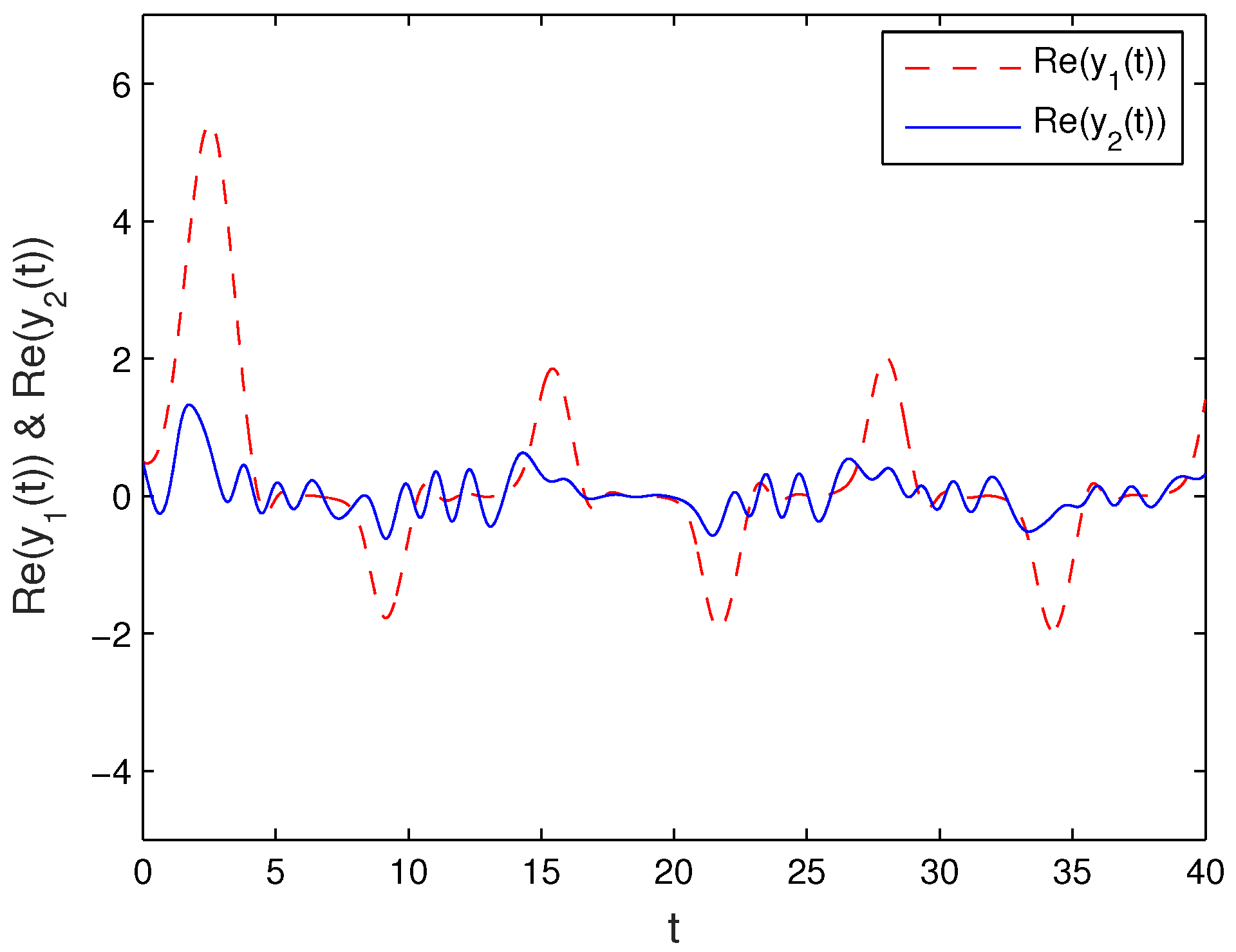
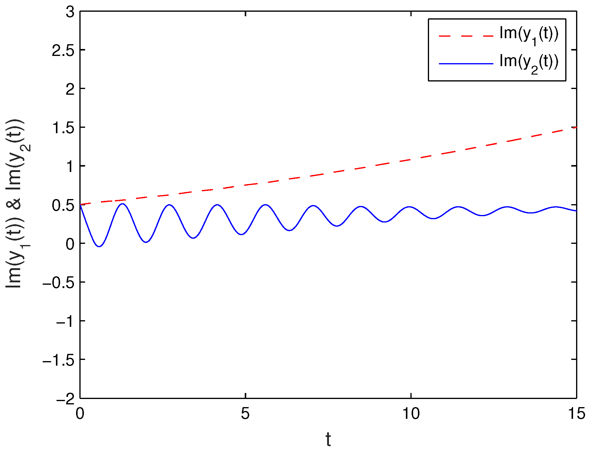
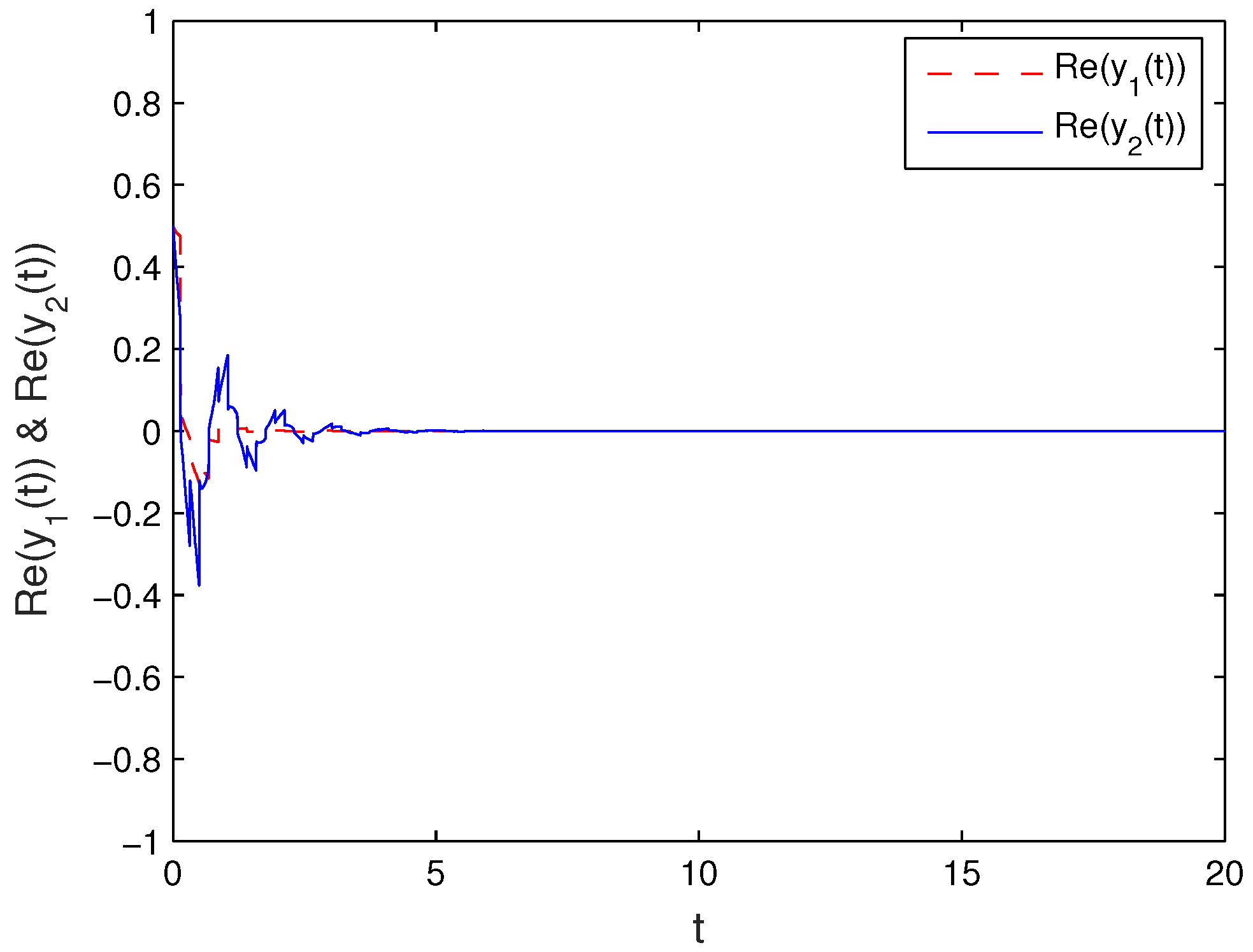
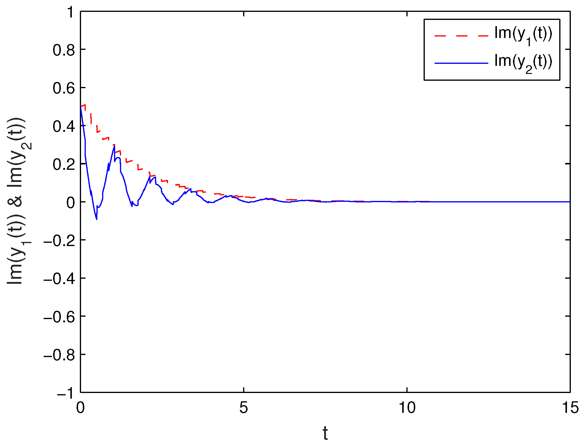
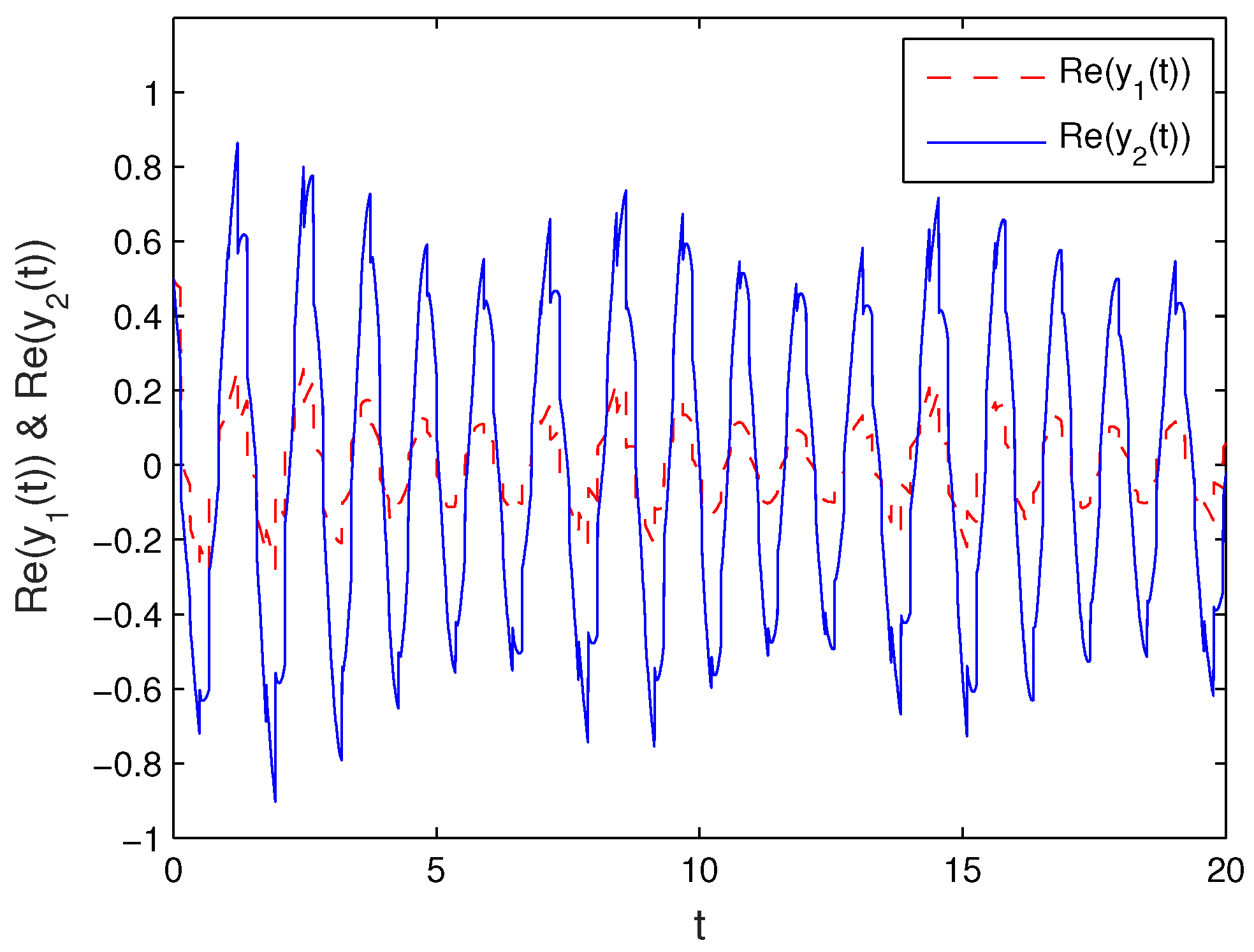
Figure 1 and Figure 2 present the state trajectories of real and imaginary parts of CVNNs (3) with initial value ${\chi }_1\left(t\right)=0.5sint+i0.5sint$, ${\chi }_2\left(t\right)=0.5cost+i0.5cost,$ which indicates that the system is unstable without impulsive control. Via the designed impulsive control, the system (3) is globally exponentially stable and the state trajectories of real and imaginary parts are shown in Figure 3 and Figure 4.

If we let:

$$Y_k=\left[\begin{array}{cc}-2.3047+0.0696i& -0.1321+0.7280i\\ -0.4270-0.3643i& -1.2465-0.0700i\end{array}\right],$$

$$Z_k=\left[\begin{array}{cc}-0.7252+0.3373i& -0.3810-0.6943i\\ -0.7257+0.4973i& -0.4498+0.3353i\end{array}\right],$$

then under the same matrices X, $\tilde{G}$, $\tilde{Q}$, $\tilde{M}$, $\widehat{G}$, $\widehat{Q}$, $\widehat{M}$ as above, LMIs (17)–(20) do not hold. The gain matrices of the control law are given by

$$E_k=\left[\begin{array}{cc}-0.6611+0.2206i& -0.0007-0.0211i\\ -0.1022+0.0212i& -0.3608-0.1104i\end{array}\right],$$

$$F_k=\left[\begin{array}{cc}-0.2024-0.2104i& -0.1004-0.1022i\\ -0.2014+0.1016i& -0.2107-0.1507i\end{array}\right].$$

It can be seen from Figure 5 and Figure 6 that the system is unstable under such impulsive control, which shows that if LMIs (17)–(20) do not hold, under derived impulsive control, the system may be unstable. It is again verified that the LMIs’ conditions in Theorem 2 are effective.

5. Conclusions

In this paper, the exponential stability for a comprehensive model of CVNNs which simultaneously contains uncertain parameters and mixed time-delays was investigated by delayed impulsive control. A new impulsive differential inequality was applied to resolve the difficulties caused by the mixed time delays and delayed impulse effects. Instead of decomposing CVNNs into real and imaginary parts, the complex Lyapunov function method has been employed to establish the stability of models, which is valid regardless of whether the activation functions can be decomposed. All the stability criteria were formulated in the form of complex-valued LIMs, which are easily checked using the Matlab LMI toolbox. Our results generalize and improve some existing results. Finally, a numerical example has been given to show the validity of the derived results. In the future, it would be an interesting research topic to study the state estimation problem of delayed CVNNs.

References

- Cohen, M.; Grossberg, S. Absolute stability of global pattern formation and parallel memory storage by competitive netural networks. IEEE Trans. Syst. Man Cybern. 1983, 13, 815–826. [Google Scholar] [CrossRef]
- Sun, L.; Tang, Y.; Wang, W.; Shen, S. Stability analysis of time-varying delay neural networks based on new integral inequalities. J. Frankl. Inst. 2020, 357, 10828–10843. [Google Scholar] [CrossRef]
- Chua, L.; Yang, L. Cellular neural networks: Theory. IEEE Trans. Circ. Syst. 1988, 35, 1257–1272. [Google Scholar] [CrossRef]
- Zeng, Z.; Zheng, W. Multistability of two kinds of recurrent neural networks with activation functions symmetrical about the origin on the phase plane. IEEE Trans. Neural Netw. Learn. Syst. 2013, 24, 1749–1762. [Google Scholar] [CrossRef]
- Hippert, H.; Pedreira, C.; Souza, R. Neural networks for short-term load forecasting: A review and evaluation. IEEE Trans. Power Syst. 2001, 16, 44–55. [Google Scholar] [CrossRef]
- Hirose, A. Complex-Valued Neural Networks, 2nd ed.; Springer: New York, NY, USA, 2012. [Google Scholar]
- Aizenberg, I. Complex-Valued Neural Networks with Multi-Valued Neurons; Springer: New York, NY, USA, 2011. [Google Scholar]
- Valle, M. Complex-valued recurrent correlation neural networks. IEEE Trans. Neural Netw. Learn. Syst. 2014, 25, 1600–1612. [Google Scholar] [CrossRef]
- Hirose, A. Generalization characteristics of complex-valued feedforward neural networks in relation to rignal coherence. IEEE Trans. Neural Netw. Learn. Syst. 2012, 23, 541–551. [Google Scholar] [CrossRef]
- Jankowski, S.; Lozowski, A.; Zurada, J. Complex-valued multistate neural associative memory. IEEE Trans. Neural Netw. 1996, 7, 1491–1496. [Google Scholar] [CrossRef]
- Arik, S. An improved robust stability result for uncertain neural networks with multiple time delays. Neural Netw. 2014, 54, 1–10. [Google Scholar] [CrossRef] [PubMed]
- Li, X.; Caraballo, T.; Rakkiyappan, R.; Han, X. On the stability of impulsive functional differential equations with infinite delays. Math. Methods Appl. Sci. 2015, 38, 3130–3140. [Google Scholar] [CrossRef] [Green Version]
- Faydasicok, O.; Arik, S. An analysis of stability of uncertain neural networks with multiple time delays. J. Frankl. Inst. 2013, 350, 1808–1826. [Google Scholar] [CrossRef]
- Li, X.; Shen, J.; Rakkiyappan, R. Persistent impulsive effects on stability of functional differential equations with finite or infinite delay. Appl. Math. Comput. 2018, 329, 14–22. [Google Scholar] [CrossRef]
- Hu, J.; Wang, J. Global stability of complex-valued recurrent neural networks with time-delays. IEEE Trans. Neural Netw. Learn. Syst. 2012, 23, 853–865. [Google Scholar] [CrossRef] [PubMed]
- Zhou, B.; Song, Q. Boundedness and complete stability of complex-valued neural networks with time delay. IEEE Trans. Neural Netw. Learn. Syst. 2013, 24, 1227–1238. [Google Scholar] [CrossRef] [PubMed]
- Gong, W.; Liang, J.; Cao, J. Matrix measure method for global exponential stability of complex-valued recurrent neural networks with time-varying delays. Neural Netw. 2015, 70, 81–89. [Google Scholar] [CrossRef] [PubMed]
- Rakkiyappan, R.; Velmurugan, G.; Li, X. Complete stability analysis of complex-valued neural networks with time delays and impulses. Neural Processing Lett. 2015, 41, 435–468. [Google Scholar] [CrossRef]
- Fang, T.; Sun, J. Further investigation on the stability of complex-valued recurrent neural networks with time delays. IEEE Trans. Neural Netw. Learn. Syst. 2014, 25, 1709–1713. [Google Scholar] [CrossRef]
- Pan, J.; Liu, X.; Xie, W. Exponential stability of a class of complex-valued neural networks with time-varying delays. Neurocomputing 2015, 164, 293–299. [Google Scholar] [CrossRef]
- Zhang, D.; Jiang, H.; Wang, J.; Yu, Z. Global stability of complex-valued recurrent neural networks with both mixed time delays and impulsive effect. Neurocomputing 2018, 282, 157–166. [Google Scholar] [CrossRef]
- Song, Q.; Yan, H.; Zhao, Z.; Liu, Y. Global exponential stability of impulsive complex-valued neural networks with both asynchronous time-varying and continuously distributed delays. Neural Netw. 2016, 81, 1–10. [Google Scholar] [CrossRef]
- Rudin, W. Real and Complex Analysis; McGraw-Hill: New York, NY, USA, 1987. [Google Scholar]
- Li, X.; Donal, O.; Haydar, A. Global exponential stabilization of impulsive neural networks with unbounded continuously distributed delays. IMA J. Appl. Math. 2015, 80, 85–99. [Google Scholar] [CrossRef]
- Lin, S.; Huang, Y.; Ren, S. Analysis and pinning control for passivity of coupled different dimensional neural networks. Neurocomputing 2018, 321, 187–200. [Google Scholar] [CrossRef]
- Zeng, D.; Zhang, R.; Park, J.; Zhong, S.; Cheng, J. Reliable stability and stabilizability for complex-valued memristive neural networks with actuator failures and aperiodic event-triggered sampled-data control. Nonlinear Anal. Hybrid Syst. 2021, 39, 100977. [Google Scholar] [CrossRef]
- Liu, A.; Huang, X.; Fan, Y.; Wang, Z. A control-interval-dependent functional for exponential stabilization of neural networks via intermittent sampled-data control. Appl. Math. Comput. 2021, 411, 126494. [Google Scholar] [CrossRef]
- Mei, J.; Jiang, M.; Wang, B.; Long, B. Finite-time parameter identification and adaptive synchronization between two chaotic neural networks. J. Frankl. Inst. 2013, 350, 1617–1633. [Google Scholar] [CrossRef]
- Peng, D.; Li, X.; Rakkiyappan, R.; Ding, Y. Stabilization of stochastic delayed systems: Event-triggered impulsive control. Appl. Math. Comput. 2021, 401, 126054. [Google Scholar] [CrossRef]
- Guan, Z.; Hill, D.; Shen, X. On hybrid impulsive and switching systems and application to nonlinear control. IEEE Trans. Autom. Control 2005, 50, 1058–1062. [Google Scholar] [CrossRef]
- Liu, X.; Zhang, K. Stabilization of nonlinear time-delay systems: Distributed-delay dependent impulsive control. Syst. Control Lett. 2018, 120, 17–22. [Google Scholar] [CrossRef]
- Li, X.; Yang, X.; Huang, T. Persistence of delayed cooperative models: Impulsive control method. Appl. Math. Comput. 2019, 342, 130–146. [Google Scholar] [CrossRef]
- Wei, L.; Chen, W.; Huang, G. Globally exponential stabilization of neural networks with mixed time delays via impulsive control. Appl. Math. Comput. 2015, 260, 10–26. [Google Scholar] [CrossRef]
- Chen, W.; Luo, S.; Zheng, W. Generating globally stable periodic solutions of delayed neural networks with periodic coefficients via impulsive control. IEEE Trans. Cybern. 2017, 47, 1590–1603. [Google Scholar] [CrossRef] [PubMed]
- Zhou, Y.; Zhang, H.; Zeng, Z. Quasi-Synchronization of Delayed Memristive Neural Networks via a Hybrid Impulsive Control. IEEE Trans. Syst. Man Cybern. Syst. 2021, 51, 1954–1965. [Google Scholar] [CrossRef]
- Zhou, Y.; Zeng, Z. Event-triggered impulsive control on quasi-synchronization of memristive neural networks with time-varying delays. Neural Netw. 2019, 110, 55–65. [Google Scholar] [CrossRef] [PubMed]
- Tang, Q.; Jian, J. Matrix measure based exponential stabilization for complex-valued inertial neural networks with time-varying delays using impulsive control. Neurocomputing 2018, 273, 251–259. [Google Scholar] [CrossRef]
- Li, X.; Fang, J.; Li, H. Master-slave exponential synchronization of delayed complex-valued memristor-based neural networks via impulsive control. Neural Netw. 2017, 93, 165–175. [Google Scholar] [CrossRef]
- Kan, Y.; Lu, J.; Qiu, J.; Kurths, J. Exponential synchronization of time-varying delayed complex-valued neural networks under hybrid impulsive controllers. Neural Netw. 2019, 114, 157–163. [Google Scholar] [CrossRef]
- Wang, Z.; Liu, X. Exponential stability of impulsive complex-valued neural networks with time delay. Math. Comput. Simul. 2019, 156, 143–157. [Google Scholar] [CrossRef]
- Zhao, Y.; Li, X.; Cao, J. Global exponential stability for impulsive systems with infinite distributed delay based on flexible impulse frequency. Appl. Math. Comput. 2020, 386, 125467. [Google Scholar] [CrossRef]
- Yang, X.; Yang, Z. Synchronization of TS fuzzy complex dynamical networks with time-varying impulsive delays and stochastic effects. Fuzzy Sets Syst. 2014, 235, 25–43. [Google Scholar] [CrossRef]
- Gunasekaran, N.; Zhai, G. Stability analysis for uncertain switched delayed complex-valued neural networks. Neurocomputing 2019, 367, 198–206. [Google Scholar] [CrossRef]
Figure 1.
Real part of state trajectories for CVNNs (3) without impulsive control.
Figure 2.
Imaginary part of state trajectories for CVNNs (3) without impulsive control.
Figure 3.
Real part of state trajectories for CVNNs (3) with time-delayed impulsive control.
Figure 4.
Imaginary part of state trajectories for CVNNs (3) with the designed impulsive controller.
Figure 5.
Real part of state trajectories for CVNNs (3) under impulsive control when LMIs (17)–(20) are not satisfied.
Figure 6.
Imaginary part of state trajectories for CVNNs (3) under impulsive control when LMIs (17)–(20) are not satisfied.
Publisher’s Note: MDPI stays neutral with regard to jurisdictional claims in published maps and institutional affiliations. |
© 2022 by the authors. Licensee MDPI, Basel, Switzerland. This article is an open access article distributed under the terms and conditions of the Creative Commons Attribution (CC BY) license (https://creativecommons.org/licenses/by/4.0/).
Share and Cite
MDPI and ACS Style
Tian, Y.; Yin, Y.; Wang, F.; Wang, K. Impulsive Control of Complex-Valued Neural Networks with Mixed Time Delays and Uncertainties. Mathematics 2022, 10, 526. https://0-doi-org.brum.beds.ac.uk/10.3390/math10030526
AMA Style
Tian Y, Yin Y, Wang F, Wang K. Impulsive Control of Complex-Valued Neural Networks with Mixed Time Delays and Uncertainties. Mathematics. 2022; 10(3):526. https://0-doi-org.brum.beds.ac.uk/10.3390/math10030526
Chicago/Turabian StyleTian, Yujuan, Yuhan Yin, Fei Wang, and Kening Wang. 2022. "Impulsive Control of Complex-Valued Neural Networks with Mixed Time Delays and Uncertainties" Mathematics 10, no. 3: 526. https://0-doi-org.brum.beds.ac.uk/10.3390/math10030526
Note that from the first issue of 2016, this journal uses article numbers instead of page numbers. See further details here.