Development of Parallel Algorithms for Intelligent Transportation Systems

Abstract

This paper deals with the creation of parallel algorithms implementing macro-and microscopic traffic flow models on modern supercomputers. High-performance computing contributes to the development of intelligent transportation systems based on information technologies and aimed at the effective regulation of traffic in large cities. As a macroscopic approach, the quasi-gas-dynamic traffic model approximated by explicit finite-difference schemes is proposed. One- and two-dimensional variants of the system are considered, and the concept of lateral velocity and different equations for obtaining it are discussed. The microscopic approach is represented by the multilane cellular automata model. The previously developed model is extended to reproduce synchronized flow in accordance with Kerner’s three-phase theory. The new version starts from the Kerner–Klenov–Schreckenberg–Wolf model and operates with the concept of the synchronization gap. Macroscopic models are relevant for determining the common characteristics of road traffic, while microscopic models are useful for a detailed description of cars’ movement. Both approaches possess inner parallelism. The parallel algorithms are based on the geometrical parallelism principle with different boundary conditions at interfaces of the subdomains. Sufficiently high speedups were reached when up to 100 processors were involved in calculations. The proposed algorithms can serve as the core of ITS.

1. Introduction

1.1. Motivation of the Research

The world experience shows that for the effective regulation of traffic in large cities it is necessary to implement an intelligent transportation system (ITS) that is actually a set of systems based on information, communication and management technologies embedded in vehicles and road infrastructure. An ITS should be able to promptly coordinate the interaction of all road users, special services and departments. Therefore, ITS combines a variety of innovative solutions, from mathematical models and methods for describing traffic to decision support systems for traffic management, not to mention the technical and engineering aspects. There are many periodicals devoted to both fundamental and practical problems of ITS. Almost all well-known publishing houses such as Elsevier, Springer, Taylor & Francis have been producing journals, Special Issues and books on this topic during the past two decades (see, e.g., [1,2,3,4,5,6]).

Nowadays, the precondition for the successful development of ITS is, on the one hand, availability of information about traffic flows from numerous cameras and sensors, and on the other hand, the existence of high-performance computing (HPC) systems allowing us to process this information, which is a huge amount of data. Promising Big Data technologies [7] with the use of massively parallel processing (MPP) systems, uniting hundreds and thousands of computational nodes, contributes to the ITS development.

Investigations proposed in this paper are directly related to the concept of ITS and the innovative urban environment “Smart City”, since the developed algorithms for MPP can serve as the core of ITS.

1.2. Research Objective

The present paper is devoted to the creation of parallel versions of algorithms for both microscopic and macroscopic traffic flow models [8].

A microscopic approach to transport modeling based on the cellular automata (CA) theory [9] has gained great popularity over the past few years. This approach allows us to take into account many technical parameters and features of the drivers’ behavior. Such models can include a detailed description of cars’ movement at intersections and in places of narrowing of roads, overtaking and changing lanes, ensuring a high degree of accuracy of the model’s correspondence to the real situation.

A separate and important task of microscopic modeling is to build a new mathematical model of traffic flows that is able to reproduce synchronized flow, and that is in agreement with Kerner’s three-phase-theory.

At the same time, macroscopic models do not lose their relevance in determining the main characteristics of road traffic, which are necessary for transport planning.

The main goal of the authors of this article is to propose parallel implementations of their original macro- and microscopic models. The models themselves have been verified previously [10,11,12]. However, parallel algorithms under development are quite general and can also be used to implement other models.

1.3. Research Methodology

A macroscopic model draws an analogy of congestion traffic flow with the gas-dynamic flow, that is, it uses the continuum approach. Namely, the model proposed by the authors is based on the quasi-gas-dynamic (QGD) system of equations [13]. The QGD system was created for solving gas-dynamic problems in a wide range of Mach numbers and has proven itself well in the simulation of supersonic, transonic, as well as subsonic flows. The traffic flow under certain conditions (congestion traffic when the strategies of all drivers are the same) can be considered as a flow of a slightly compressible fluid and vehicles’ motion can be described by equations similar to the equations of gas dynamics. Therefore, it seemed natural to adapt the QGD system to simulate traffic flows by introducing terms into the equations that allow us to take into account the peculiarities of the drivers’ behavior—the so-called human factor.

The main specialty of the proposed QGD traffic model is that it is two-dimensional and, thanks to the introduction of lateral velocity, allows describing traffic on the road, taking into account its real geometry.

The introduced microscopic model uses the cellular automata ideology [9]. The paper reports an original two-dimensional CA model, which is a generalization of the Nagel–Schreckenberg model [14] for the multilane case. For this model, algorithms have been built that describe the real behavior of drivers [15]. Additionally, the paper, for the first time, presents a new version of the CA model starting from the Kerner–Klenov–Schreckenberg–Wolf model [16].

Both macro- and micro-approaches possess inner parallelism and are suitable for fast calculations on supercomputers, even for modeling large-scale road networks with several million vehicles.

In order to obtain efficient parallel implementations, a certain methodology known as Ian Foster’s PCAM (Partitioning, Communication, Agglomeration and Mapping) concept [17] is applied. It means partitioning the problem into tasks (for example, domain or functional decomposition), identifying the necessary communication between the tasks, agglomeration of fine-grained tasks into fewer coarse-grained tasks and finally mapping coarse-grained tasks to processors in the most rational way to achieve good load balancing.

Both the QGD traffic model and the CA model use domain decomposition (the data parallelism) as the partitioning technique. Note that in Russian-language scientific literature, such partitioning is often called geometric parallelism. When simulating traffic, the road network is a computational domain that is geometrically split into parts, and calculations are performed concurrently in these sub-domains. The principles of splitting are different for the macroscopic and CA models; they are discussed in the corresponding sections of the paper. In any case, local communication involving only neighboring sub-domains is realized. Agglomeration and mapping aiming at good scaling and efficiency of the code depend on details of the problem and also on the MPP system available.

Among the possible algorithms of macroscopic model numerical implementation, explicit finite-difference schemes for the equation approximation seem to be the most promising. They are logically simple algorithms and can be parallelized using domain decomposition (distribution of points of the computational grid across computer nodes, including CPU and GPU cores) with the minimum of local communication. As a rule, explicit schemes demonstrate good scalability and portability in a wide range of supercomputer architectures. Therefore, conservative explicit finite-difference schemes were chosen for the QGD traffic model implementation.

1.4. Scientific Contribution

The main scientific contributions are:

-

Macroscopic two-dimensional QGD model for traffic flow simulation including lateral velocity of lane change; two different forms for lateral velocity with recommendations for their use;

-

A special form of internal boundary conditions for their exchange at the boundaries of subdomains;

-

A multilane CA model with speed adaptation mechanisms featuring various driving strategies;

-

Parallel implementation of traffic flow models based on the domain decomposition technique and adapted to HPC systems with distributed memory.

The paper is organized as follows. Section 2 provides an overview of the current state of the research field. Section 3 presents the macroscopic quasi-gas-dynamic traffic model, a parallel algorithm of its implementation and results of numerical experiments. Section 4 proposes speed adaptation algorithms for the new cellular automata traffic flow model, as well as discusses its parallel implementation. Section 5 concludes the paper with some discussions and conclusions.

2. State of the Art in the Research Field

The traffic flow simulation in its modern concept began in the middle of the 20th century. At that time, the research moved towards the creation of models that would allow reproducing the main features of traffic flows [18,19,20,21]. Investigations were carried out both in the direction of macroscopic and microscopic modeling. Over time, models appeared that took into account the human factor and reproduced the movement of individual car–driver particles.

The first macroscopic model is the well-know LWR model introduced by Lighthill and Whitham in 1955 [18]. Later, higher-order models appeared, containing an equation for acceleration of various types. The first simple model derived in 1971 from the car-following model was Payne macroscopic model [19]. Philips in 1979 proposed the model in which system contains mass, momentum and energy conservation equations [22]. The model considering sound speed and viscosity was developed by Kuehne in 1984 [23]. The phenomenological model of Kerner–Konhaeuser [24] is also well known.

Much effort has gone into making macro models anisotropic. This means that cars should only react to the situation in front of them. The most well-known model that resolves this problem is the Aw and Rascle model [25].

Modern studies of traffic flow dynamics are basically aimed at complicating the existing models. An example is the following publications devoted to macroscopic models of the hydrodynamic type.

The authors of the article [26] propose a new lattice-model, with the help of which they investigate how the driver’s memory volume affects the dynamics of the traffic flow. Linear stability analysis shows that the temporal length of the driver’s memory has a significant influence on the stability of traffic flow. In the article [27] of the same authors, an extended one-dimensional hydrodynamic lattice model is proposed to study the flow dynamics when driving on a curved road. The result of the analysis shows that the radian of a curved road plays an important role in influencing the flow stability. The authors of the paper [28] use the hydrodynamical approach to describe the traffic flow over the crossroad, taking into account the traffic light regimes. The article [29] examines the impact of driver behavior on driving on a curved road using also the hydrodynamic lattice approach.

In the field of micro-simulation the progressive trend is modeling based on the cellular automata theory. The first model in this field was developed by Cremer and Ludwig [30]. The model considered classical was proposed in 1992 by Nagel and Schreckenberg [14]. Later, models with more complex algorithms appeared, for example, allowing us to reflect the three-phase theory of Kerner [16]. Nowadays, the models of this type remain one of the principal directions of transport modeling [9,31,32,33,34].

In recent years, the volume of traffic has increased several times, which makes it necessary to use computer systems of super-high performance for adequate modeling with the ability to carry out real-time calculations. It should be noted that models of both types can be efficiently employed to simulate traffic on large road networks due to the capacity of modern supercomputers.

The TOP500 rating [35] presents the list of the most powerful general purpose systems that are in common use for high end applications. Computers are ranked by their performance on the High-Performance Linpack (HPL) benchmark [36], not by their peak performance. The world is waiting for the first “Exascale” system—the appearance of such a system by 2021 has been predicted, but this has not happened yet. The present 58th edition of the list was published in November 2021. The system, named Fugaku, manufactured by Fujitsu and installed at RIKEN Center for Computational Science in Kobe, Japan, remains No. 1. It has 7,630,848 cores, which allowed it to achieve an HPL benchmark score of 442 Petaflop/s. Additionally, this is nearly half of Exaflop/s, which is ultra-high performance! This is a rare example of a supercomputer based on traditional CPU-only architecture, while most of the supercomputers on the list have hybrid architectures and include various computing accelerators, mainly GPUs.

There are various problems of using the full potential of MPP systems. Among them, there are the problems of energy efficiency, fault tolerance, and scalability and portability of computational algorithms. For example, hybrid architecture systems are more energy efficient, but the programming for such systems is laborious, since the application development must be architecture-oriented to achieve high parallelization efficiency. In this sense, from the two approaches to modeling traffic flows discussed in the present article, macroscopic models look more promising when they are implemented by explicit finite-difference methods. Microscopic models of cellular automata based on logical operations are difficult to parallelize on graphics accelerators. To implement them, MPP systems of a more traditional architecture are chosen or only the CPU cores of hybrid systems are used.

The present work corresponds to modern scientific trends in the field of traffic simulation and parallel algorithm design. It is comparable with the achievements of other research teams as evidenced by the publications cited.

3. Macroscopic Quasi-Gas-Dynamic Traffic Model

3.1. Governing Equations

As a basis for the development of a parallel macroscopic algorithm, a gas-dynamic model proposed by the authors earlier was used [10]. This model belongs to the higher-order type of macroscopic traffic models.

In the one-dimensional case in terms of flux (Q) and density (ρ) the system of equations looks like this:

$$\frac{\partial \rho }{\partial t}+\frac{\partial Q}{\partial x}=\frac{\partial }{\partial x}\frac{\tau }{2}\frac{\partial \left(\frac{Q^2}{\rho }+P\right)}{\partial x}+F_{\rho },$$

(1)

$$\frac{\partial Q}{\partial t}+\frac{\partial }{\partial x}\left[\frac{Q^2}{\rho }+P\right]=f+\frac{\partial }{\partial x}\frac{\tau }{2}\frac{\partial \left(\frac{Q^3}{{\rho }^2}+P\frac{Q}{\rho }\right)}{\partial x}+F_U.$$

(2)

Here, τ is the small parameter interpreted as a reference time (the time interval in which several vehicles cross a given point of the road). $F_{\rho }$ and $F_U$ are the source functions, which are not equal to zero at points of the road heterogeneity, that is, in the presence of on-rump or off-rump or in case of changes in the number of lanes on the highway.

The equations use the space-averaged quantities $\rho \left[\mathrm{vehicles}/\mathrm{km}/\mathrm{lane}\right]$ and $Q\left[\mathrm{vehicles}/\mathrm{hour}/\mathrm{lane}\right]=\rho \cdot U\left[\mathrm{km}/\mathrm{hour}\right]$, and the analogue of pressure (traffic pressure) $P=\lambda {\rho }^{\beta }/\beta$.

Compared to gas dynamics, the additional terms are as follows:

-

Acceleration/deceleration force $f=a\cdot \rho$,

-

Acceleration $a=\left(U_{eq}-U\right)/T$,

-

Equilibrium speed $U_{eq}=U_{free}\left(1-\rho /{\rho }_{jam}\right)$,

-

Relaxation time $T=t_0\left(1+r\rho /\left({\rho }_{jam}-r\rho \right)\right),$ $r,t_0$—phenomenological constants.

There is a two-dimensional version of the QGD traffic model to account for real road geometries. A feature of the proposed model is the introduction into the number of primary variables the lateral velocity, which describes the speed of lane change in case of multilane traffic. Vehicles can move into a lane with a lower density or higher speed or change the lane if it helps to reach a certain target, for example, to leave the highway.

There are different ways of representing this variable.

It would be natural to introduce formulae for the forward (U) and lateral (V) velocities in a similar way by analogy with two velocity components in the QGD system. Then, the two-dimensional system of equations would look like this:

$$\begin{array}{l}\frac{\partial \rho }{\partial t}+\frac{\partial }{\partial x}\left(\rho U\right)+\frac{\partial }{\partial y}\left(\rho V\right)\\ =\frac{\partial }{\partial x}\frac{{\tau }_x}{2}\left(\frac{\partial }{\partial x}\left(\rho U^2+P_x\right)-f_x+\frac{\partial }{\partial y}\left(\rho UV\right)\right)+\frac{\partial }{\partial y}\frac{{\tau }_y}{2}\left(\frac{\partial }{\partial y}\left(\rho V^2+P_y\right)-f_y+\frac{\partial }{\partial x}\left(\rho UV\right)\right),\end{array}$$

(3)

$$\begin{array}{l}\frac{\partial \rho U}{\partial t}+\frac{\partial }{\partial x}\left(\rho U^2+P_x\right)-f_x+\frac{\partial }{\partial y}\left(\rho UV\right)\\ =\frac{\partial }{\partial x}\frac{{\tau }_x}{2}\left(\frac{\partial }{\partial x}\left(\rho U^3+3P_{x}U\right)-3f_{x}U\right)+\frac{\partial }{\partial y}\frac{{\tau }_y}{2}\left(\frac{\partial }{\partial y}\left(\rho U{V}^2+P_{y}U\right)-f_{y}U\right)\\ +\frac{\partial }{\partial x}\frac{{\tau }_x}{2}\left(\frac{\partial }{\partial y}\left(\rho U^{2}V+P_{y}V\right)-f_{y}V\right)+\frac{\partial }{\partial y}\frac{{\tau }_y}{2}\left(\frac{\partial }{\partial x}\left(\rho U^{2}V+P_{x}V\right)-f_{x}V\right),\end{array}$$

(4)

$$\begin{array}{l}\frac{\partial \rho V}{\partial t}+\frac{\partial }{\partial y}\left(\rho V^2+P_y\right)-f_y+\frac{\partial }{\partial x}\left(\rho UV\right)\\ =\frac{\partial }{\partial x}\frac{{\tau }_x}{2}\left(\frac{\partial }{\partial x}\left(\rho U^{2}V+P_{x}V\right)-f_{x}V\right)+\frac{\partial }{\partial y}\frac{{\tau }_y}{2}\left(\frac{\partial }{\partial y}\left(\rho V^3+3P_{y}V\right)-3f_{y}V\right)\\ +\frac{\partial }{\partial x}\frac{{\tau }_x}{2}\left(\frac{\partial }{\partial y}\left(\rho V^{2}U+P_{y}U\right)-f_{y}U\right)+\frac{\partial }{\partial y}\frac{{\tau }_y}{2}\left(\frac{\partial }{\partial x}\left(\rho V^{2}U+P_{x}U\right)-f_{x}U\right).\end{array}$$

(5)

The corresponding components in Equations (2) and (3) are calculated in a similar manner. The acceleration/deceleration forces f_x and f_y are determined through the forward and lateral velocities, respectively. As the equilibrium lateral velocity $V_{eq}$ in function f_y, one can take the next velocity $V_l$:

$$V_l=k_u\rho \frac{\partial U}{\partial y}-k_{\rho }U\frac{\partial \rho }{\partial y}+k_{des}\frac{U^2}{{\left(x_{des}-x\right)}^2}\left(y_{des}-y\right),$$

(6)

where each term represents one of the three desires of the driver described above. Here, $k_u,k_{\rho },k_{des}$ are some constants, and $\left(x_{des},y_{des}\right)$ are coordinates of the desired destination.

At the same time, algebraic Equation (6) can be used itself instead of Equation (5) to obtain the lateral velocity, thus we simplify the numerical implementation.

An explicit finite difference method was used for the calculations. Spatial derivatives in the partial differential equations were approximated by central differences of the second order of approximation. The conditional stability of the schemes is ensured by the presence of diffusion terms with small parameters in the right hand sides of (3)–(5), mixed derivatives can be neglected.

To check both approaches, the test problem about the movement along the road with an entrance has been solved. Calculations have shown that the solution based on system (3)–(5) requires a much smaller time step to maintain the stability—approximately by two orders of magnitude compared to the approach without differential Equation (5). At the same time, the solutions themselves practically do not differ from each other. Therefore, it is more rational and economical to use Equation (6) for obtaining the lateral velocity in real predictive modeling.

The 2D QGD traffic model in formulation (3), (4), (6) was verified by numerous test predictions and compared with the multilane CA model [10,11]. Quasi-one-dimensional calculations made it possible to compare this formulation with 1D models of other authors. Some problems discussed in [8] were used for numerical experiments. Formulation (1)–(2) was compared with LWR model with diffusion and source terms in the right hand side of the continuity equation. Traffic was simulated on roads with rather complex geometry [12]. In all cases, a qualitative agreement of the results was obtained. The analysis of the results allowed us to conclude that the QGD traffic model reproduces the main patterns of traffic flows well.

3.2. Parallel Implementation

It is obvious that the goal of parallel computing is to minimize the total execution time, and the most efficient parallelization strategy for each problem generally requires a unique solution. However, despite the variety of the solutions, it is possible to identify some basics of parallel algorithm design, for example, Ian Foster’s PCAM concept is such a regulation [17]. Sometimes it is difficult for software developers to distinguish between the Partitioning, Communication, Agglomeration and Mapping stages, and they intuitively go through these stages when aiming for a highly scalable algorithm and good load balancing.

If we talk about explicit finite-difference methods for the numerical solution of partial differential equations, then their parallelization techniques are well developed: they are simple and highly efficient. Partitioning means the computational domain decomposition. As calculations in all inner points of the computational grid are identical and can be performed concurrently needing local communications only with neighboring points, fine-grained tasks here are tasks in each point of the domain. Of course, they should agglomerate into fewer coarse-grained tasks of larger size in order to decrease the ratio of the volume of communication to the volume of computation. At this stage, we must take into account the details of the problem under consideration. The next stage—mapping—requires taking into account also the features of the MPP system used.

In this regard, we would like to mention the experience of supercomputer modeling of complex fluid flows in a porous medium using hybrid clusters [37]: the authors created a procedure of automatic data distribution among processing units (CPU cores or GPUs) to ensure optimal load balancing depending on a priori estimation of the run time for each possible configuration. Computational complexity of porous medium flow problems, hardware performance, latency and data exchange time were evaluated empirically and included in the formula to estimate the run time.

The numerical implementation of the QGD traffic model is based on explicit methods, therefore the above remarks are valid. The parallelization technique focuses on distributed memory and message passing.

The computational domain, that is, the road network, is divided into approximately equal segments approximately equal in the number of computational grid points for uniform loading of processors (assuming the homogeneity of a multiprocessor system). It is natural to split the road network into segments (straight sections of roads that may contain narrowings/widenings, side entrances/exits) connecting intersections, which are the network nodes. These segments are sub-domains covered by the 2D Cartesian computational grid. As the number of grid points in the x-direction (the direction of the forward velocity) is much greater than in the y-direction (across the road) the grid is never split along the y-direction, but long road sections can be additionally split along the x-direction if necessary. As an example, Figure 1 reflects decomposition of a small road network with one-way traffic into twelve segments (s_i denotes the i-th segment, and, what is the same, the i-th sub-domain, i = 1, …, 12), and arrows indicate the direction of the forward velocity. In the case of two-way traffic, road segments in different directions should be different sub-domains.

The network nodes are boundaries of computational sub-domains, and boundary conditions should be set at the boundary and near-boundary points, observing the conditions for the conservation of mass and fluxes in neighboring areas. For example, if the intersection consists of N incoming and one outgoing road segments, the density at the boundary of the outgoing flow is equal to the sum of the incoming flow densities:

$${\rho }_{out}\left(x_B,t\right)={\displaystyle \sum _{i=1}^N{\rho }_{ini}\left(x_B,t\right)}.$$

(7)

To set the velocities at the boundaries, the scheme with weights is used:

$$U_{out}\left(x_B,t\right)={\displaystyle \sum _{i=1}^2{w}_i{U}_{ini}\left(x_B,t\right),w_i=\frac{{\rho }_{ini}\left(x_B,t\right)}{{\rho }_{out}\left(x_B,t\right)}}.$$

(8)

There are no calculations, but only communications in intersections: neighboring sub-domains exchange the values of densities and velocities included in (7) and (8). The number of lanes in neighboring road segments can be different, but the number of grid points in the y-direction should match to facilitate implementation of the boundary conditions.

Thus, we cover the Partitioning, Communication and Agglomeration stages of Foster’s paradigm as a whole.

As for the Mapping stage, each sub-domain is processed by a separate processing unit, more precisely, by a core of CPU. It does not matter whether the employed cores belong to the same node of the MPP system or are physically distributed throughout the system.

The parallel code is written in C/C++ with the use of MPI to support communication.

3.3. Numerical Results

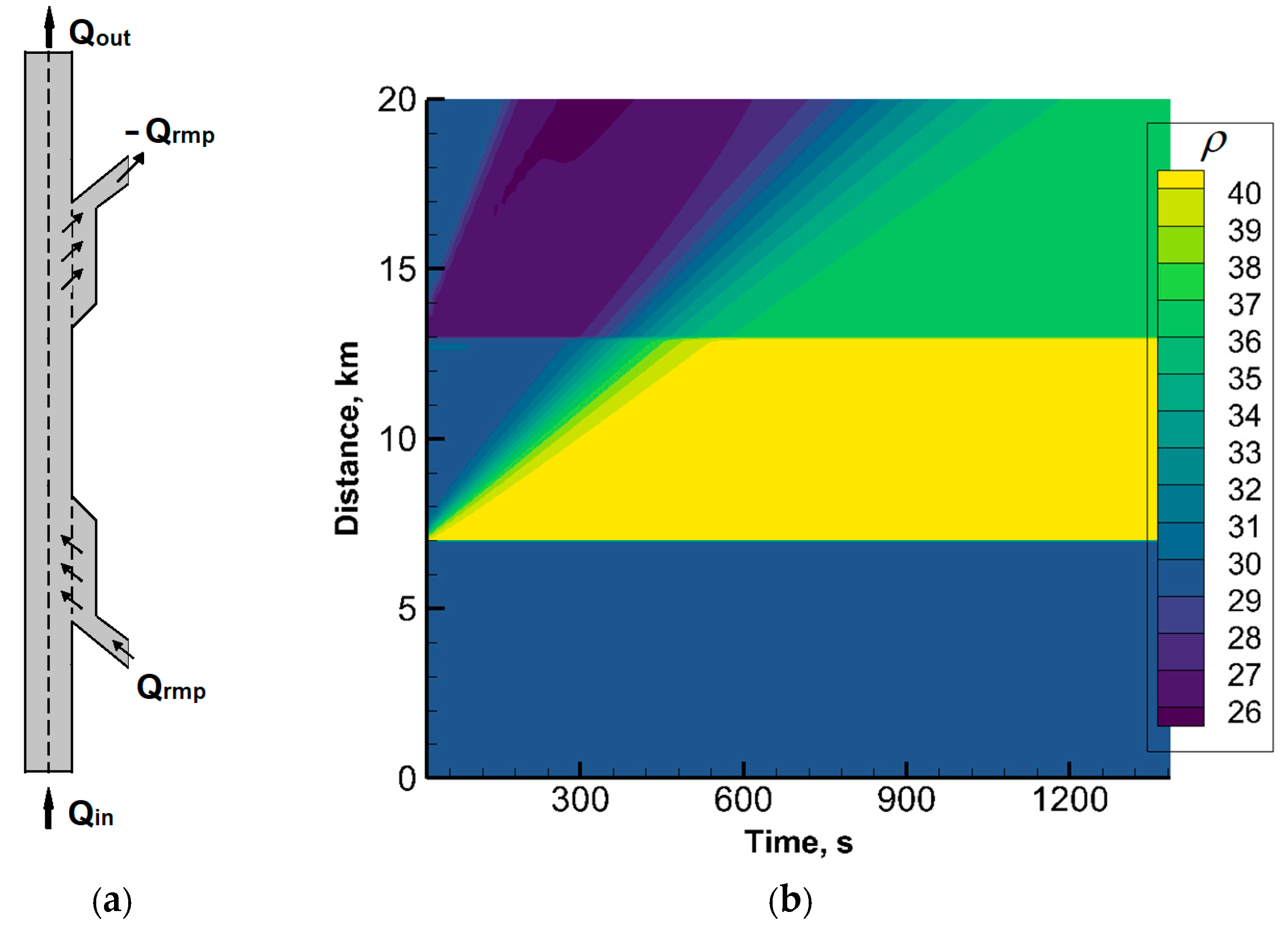
For experimental investigation of software scalability and efficiency of the proposed parallel algorithm, the test problem of traffic on a highway with an on-ramp and off-ramp in the multi-lane setting was solved numerically (see Figure 2a).

The initial density is quite low: ρ_init = 30 vehicles/km/lane.

Fluxes Q_in and Q_rmp are constant, $Q_{rmp}=(C-Q_{in})/2$, where C is the road capacity.

The spatiotemporal diagram of the obtained effective density is depicted in Figure 2b. Comparison with similar problems from [8] allows us to conclude that the sample demonstrates the impact of bottlenecks correctly.

There are two common types of scaling: strong and weak scaling. Strong scaling is associated with Amdahl’s law, which gives the upper limit of speedup for a problem of fixed size. While weak scaling is associated with Gustafson’s law, which states no upper limit for the scaled speedup. This scaled speedup is calculated based on the amount of work done for a scaled problem size (in contrast to Amdahl’s law) [17]. Thus, the method of increasing the problem size in proportion to the increase in the number of processors is usually used to evaluate weak scaling. However, we are interested in strong scaling, therefore we split one and the same sufficiently fine computational grid in our experiments.

The computational domain covered by the grid of $10.000\times 300=3\mathrm{million}$ points was split into sub-domains along the x-direction according to the number of engaged processors. Calculations were performed on the K100 supercomputer with the peak performance of 100 Teraflop/s installed in Keldysh Institute of Applied Mathematics (KIAM). Each node of K100 consists of two CPUs (Intel Xeon X5670) with 12 cores available to the user’s task. Up to 100 CPU cores from different nodes have been involved in calculations. GPUs have not been used in the computation.

To estimate the speedup the run time of 100 time levels of our explicit difference scheme was measured for each number of CPU cores used.

On one core it was 26.67 s,

On 5 cores—9.4 s,

On 100 cores—0.71 s.

Note that this is a very small part of the entire calculation, which, in principle, can take place indefinitely in real-time. The run time analysis shows not quite satisfactory speedup.

Some tuning work was carried out to achieve better speedup: the number of exchange operations between sub-domains and the volume of data transferred were reduced that resulted in a reduction of the run time on a large number of cores. One can compare speedups of the initial code and the version with message passing optimization depicted in Figure 3a,b, respectively.

The speedup in Figure 3b is nearly linear, which indicates the good scalability of the algorithm. This is typical for the parallel implementation of explicit numerical methods. Note, that as a unit the run time on 5 CPU cores is used. Thus, the figure corresponds to the parallelization efficiency of about 80 per cent on 100 cores that is high enough efficiency for the considered class of problems in the given conditions.

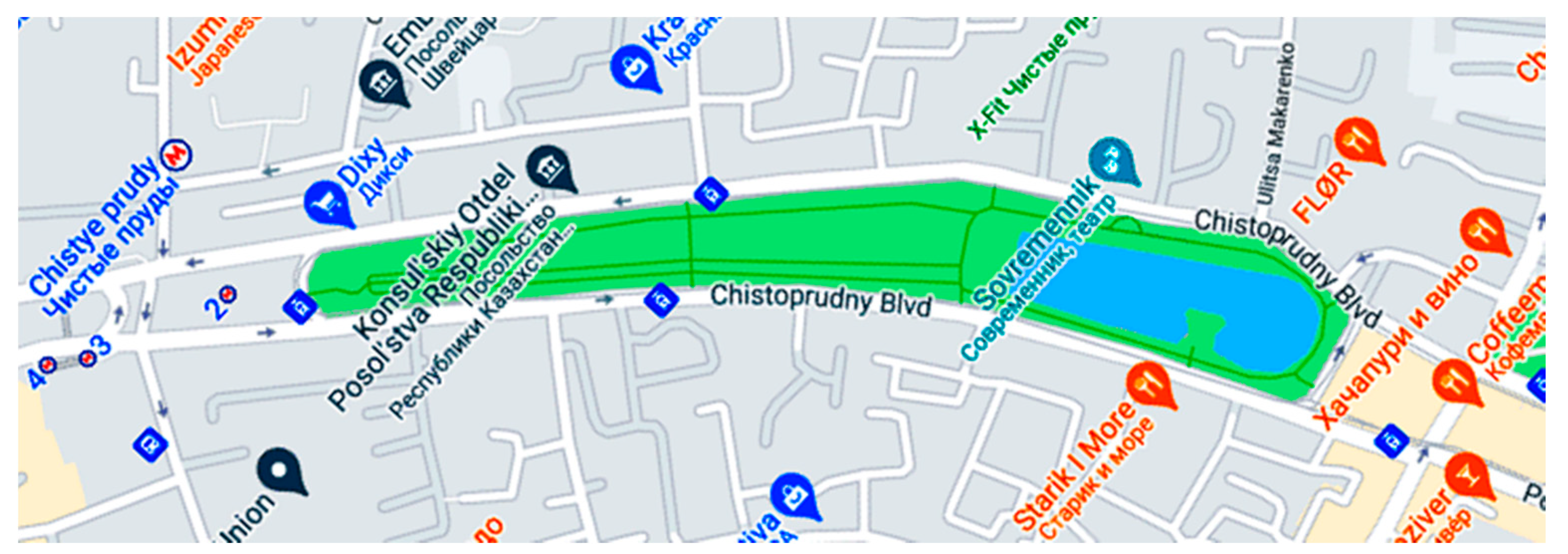
More complicated road geometry was used to demonstrate the possibility of practical application of the parallel algorithm implementing QGD traffic model. A section of the Moscow road network located near Chistoprudny Boulevard was taken for the simulation, Figure 4 shows the corresponding map fragment. Traffic on the roads under consideration is one-way.

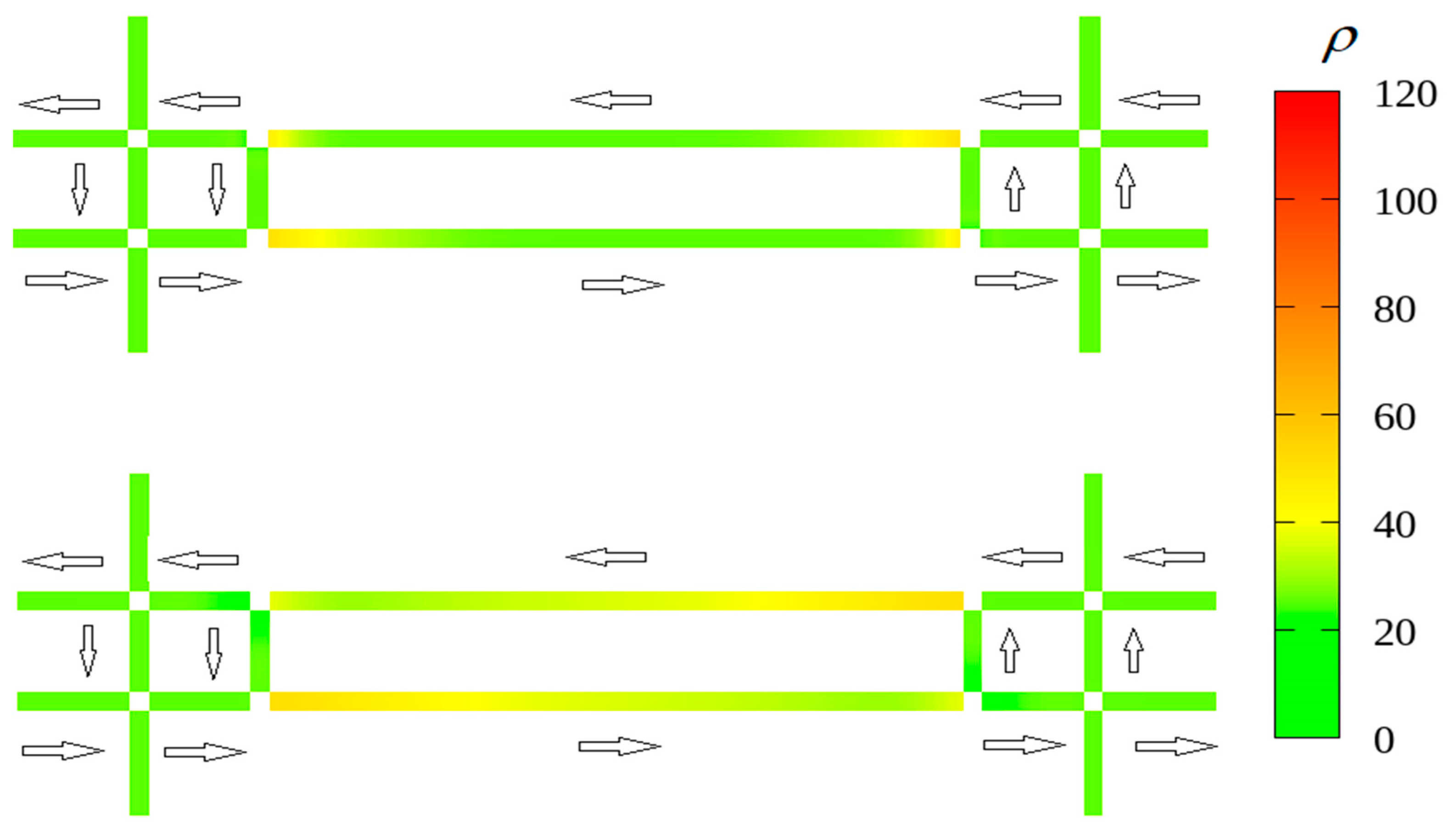
Figure 5 presents the obtained effective density fields for two successive time moments. Arrows indicate the direction of movement on road segments, which are processed by different processors like it is illustrated by Figure 1. Boundary conditions (7) and (8) are satisfied in all nodes. In this case, fluxes in all nodes are distributed uniformly.

One can see that on segments adjacent to X-crosses, the density does not change with time, but on segments adjacent to T-crosses quite logical dynamics of the density is observed.

4. Cellular Automata Approach: From Nagel–Schreckenberg-Based to KKSW-Based Model

4.1. Methods of Modeling Traffic within Cellular Automata (CA) Approach and Their Problems

Since, nowadays, quite a large amount of data from cameras and detectors is accumulated, we now know more than ever about the properties of traffic flows. Therefore, modern traffic flow models are required to be precise in terms of depicting the known experimental patterns, for example, those that appear for average velocities in space-time diagrams.

As is stated by B. Kerner in his three-phase traffic theory [38], there are three phases in a vehicular flow: free flow, synchronized flow and wide moving jam. Several things should be noted regarding the transitions between these phases. First, they appear consequently, i.e., free flow transits to synchronized flow (F-S transition), and synchronized flow transits to wide moving jam phase (S-J transition). F-J transitions do not occur without the S phase in between, according to Kerner’s theory, which is based strictly on experimental data. While different models have their own problems depicting these phases and transitions, it is known that the original Nagel–Schreckenberg model [14], as well as many of its successors developed later, does not reproduce the synchronized flow. The reason behind it is quite straight-forward: vehicles do not adjust their speed to the ones in front of them, they speed up until the point where they catch up with the leader, only slowing down when it is necessary to avoid collision. On the other hand, the hysteresis effect known to occur in transitions, when the same density of the vehicles on a road can result in different phases of traffic (F and S, or S and J) due to stochastic processes within the flow, requires two contradicting components to be included in the model: over-acceleration and speed adaptation.

In recent years the original mathematical model of traffic flows based on the cellular automata approach (CAM-2D model) has been developed by the authors of the article [12,39,40]. The main focus of the model was to depict various driving tactics as well as building algorithms for vehicle movement on different road elements, such as signalized and non-signalized intersections, road widening, U-turns, etc. Another aspect of the said work was to create parallel algorithms for this model, designed to allow carrying out computations on various road networks of cities.

The CAM-2D model is based on Nagel–Schreckenberg [14] model: while it is multilane and the set of lane changing algorithms has been added, the algorithm of moving along the road has stayed pretty much the same. While this configuration provides over-acceleration, both within the lane and due to lane changing, it lacks steps to depict the speed adaptation. The goal of this research is to build a new mathematical model of traffic flows that is able to reproduce synchronized flow and that is in an agreement with Kerner’s three-phase theory. The model that was considered as a starting point for this work is the KKSW (Kerner–Klenov–Schreckenberg–Wolf) model [16].

4.2. The Basics of the Original CA-Based Model (CAM-2D)

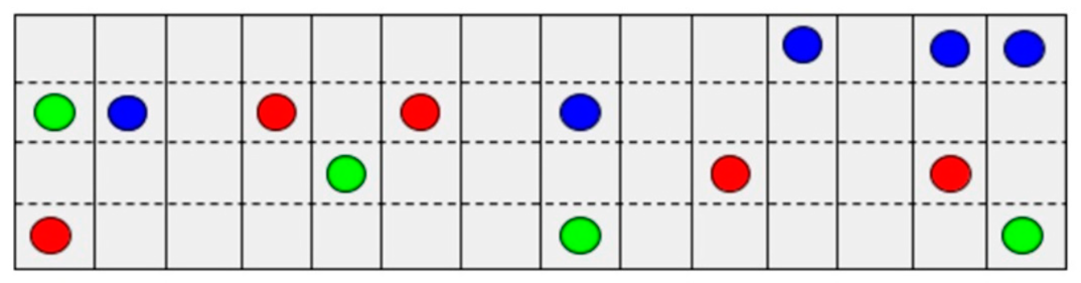
The main rationale behind the cellular automata approach in application to traffic flow modeling is discretization. The road is divided into equal cells, each either containing a single car or being empty. The cell size is 7.5 m long and one lane (approximately 3–4 m) wide. The distance in the system is measured in the number of cells. Time is also discrete, time step is equal to 1 s. Vehicle speed is measured in cells per time step and can take on values from zero to 4, which corresponds to 108 km/h. The computational domain is represented in Figure 6. Colored circles represent cars, color corresponds to their desired destination.

Each time step cell state update is carried out according to the following rules:

• Vehicles change lanes if it is necessary (to reach the desired destination or to drive around an obstacle), it is advantageous for the drivers (leads to speed increase and/or density decrease) and it is possible (i.e., if the lane change is allowed and the target cell is empty);
• Vehicles move along the road according to the classic rules of one-lane traffic.

The lane change algorithm is a complicated set of rules that varies for different road elements, different priority rules, traffic signs and road marking. It is also different for different types of drivers, distinguishing driving strategies (for details, see [15]). Drivers in the system can be cautious or aggressive, and the degree of these properties can also vary. In some situations drivers can become cooperative, reacting to the others wish to change lanes or enter the road by slowing down and letting them pass. The decision to change lanes also depends on the traffic situation both in the current and the goal lanes.

The algorithm for movement along the road is based on the four rules of the Nagel–Schreckenberg model:

• Acceleration: V_n = max (V_n + 1, V_max);
• Braking in order to avoid collisions: V_n = min (V_n, d_n − 1);
• Stochastic braking: V_n = max (V_n − 1, 0) with probability p;
• Moving along the road: X_n = X_n + V_n.

Here, V_n is the current speed of the n-th vehicle in the system, V_max is the maximal speed for these conditions, d_n is the distance between the n-th car and the one in front of it. X_n is the number of cells that the car should move forward on this time step.

4.3. Adding Speed Adaptation Steps to CAM-2D Model

The assumption behind the speed adaptation rules implemented in modern CA-based models such as KKSW, is that there is a synchronization distance G_n (which, generally speaking, depends on the velocity of a vehicle, G_n = G_n (V_n)) within which a car is willing to adjust its speed to the speed of the leader. Therefore, we expand the model adding the synchronization gap, which brings us to the general set of steps that describes the system evolution at each time step:

• Lane changing if necessary and possible;
• If the car is within the synchronization gap G_n (distance between the car under consideration and its leading car d_n ≤ G_n) then the vehicle speed V_n = V_n + sgn (V_ln − V_n), where V_ln is the leader’s speed;

Additionally, If V_n > V_ln, V_n = max (V_n + 1, V_max) with probability p₁, which describes stochastic over-acceleration within the synchronization gap distance. Here, V_max is maximal speed in the system;

3.

If the distance between the car and the leader d_n > G_n,, the car accelerates if its speed is still lower than maximal: V_n = max (V_n + 1, V_max);

4.

Braking in order to avoid collisions: V_n = min (V_n, d_n − 1);

5.

Stochastic braking V_n = max (V_n − 1, 0) with probability p;

6.

Moving along the road: X_n = X_n +V_n.

Step 1, the lane changing algorithm, is a complex set of steps that varies for different situations and different driving strategies and is developed by the authors of the article earlier (see, for example, [15]). Steps 2–6 are the same as in the KKSW model, and steps 3–6 are the same as in the classic Nagel–Schreckenberg model.

4.4. Additional Speed Adaptation for the Case of Traffic Jams in Neighbouring Lanes

This algorithm is based on the suggestion that drivers slow down if they see that there is a jam in the neighboring lane. This is a recommended course of action to provide safer driving and is usually implemented by most of the drivers. It also contributes to the overall speed adaptation effects that we seek.

To achieve this, steps 2 and 3 of the cell state update algorithm listed above have to be rewritten as follows:

Each step two parameters, jcr and jcl (“jam count right” and “jam count left”, number of vehicles in neighboring lanes, right and left accordingly, that are not moving, Vi = 0).

• If jcr > J or jcl > J, jam = true. Here, J is a parameter that should be chosen according to the task requirements during the calibration process, jam is a Boolean variable that indicates traffic jam.
• If the car is within the synchronization gap G_n (distance between the car under consideration and its leading car d_n ≤ G_n);
  if V_ln − V_n > 0 and jam = false, V_n = max (V_n + 1, V_max);
  if V_ln − V_n > 0 and jam = true, V_n = V_n;
  if V_ln − V_n = 0, V_n = V_n;
  if V_ln − V_n < 0, V_n = max (V_n − 1, 0).

Additionally, If V_ln − V_n < 0, V_n = max (V_n + 1, V_max) with probability p₁ (stochastic over-acceleration within the synchronization gap distance)_.

Here, V_n is current speed, V_ln is leader’s speed, V_max is maximal speed in the system;

3.

If the distance between the car and the leader d_n > G_n,

if jam = false, V_n = max (V_n + 1, V_max);

if jam = true, V_n = V_n.

Test computations were carried out using both algorithms to verify them, although computations using real data for model calibration and comparison are yet to be executed.

4.5. Parallel Implementation

The created model possessed inner parallelism, both geometrical and a parallelism of data, therefore the approach to developing the parallel computational algorithm for the created model can be flexible. As the first step the geometrical approach was chosen, similarly to the one developed for the CAM-2D model.

Since the main goal of the created program package is to be able to simulate traffic on various road networks it was necessary to create universal elements from which any road configuration can be obtained. They also should be interchangeable in the system, which means that, first, they should be standard size, and second, their boundaries should not contain any singularities, such as intersections, widenings, etc. The size of a single element was chosen to be 31 × 31 cells, or 232.5 × 232.5 m, representing approximately average distance between intersections in a city. In the case of longer road stretches without intersections the distance is filled with the necessary amount of straight road elements. If there is the need to model a more dense and complicated network, the size can also be decreased. Technically, it is limited only by a number of lanes on a road, but one should also be mindful that some logical operations representing driver behavior need some space within the element to take place. For example, in case of turning on an intersection, the driver might need to change lanes in order to do so, and might not be able to do so immediately. If the road network is not branched, the element size can be increased accordingly.

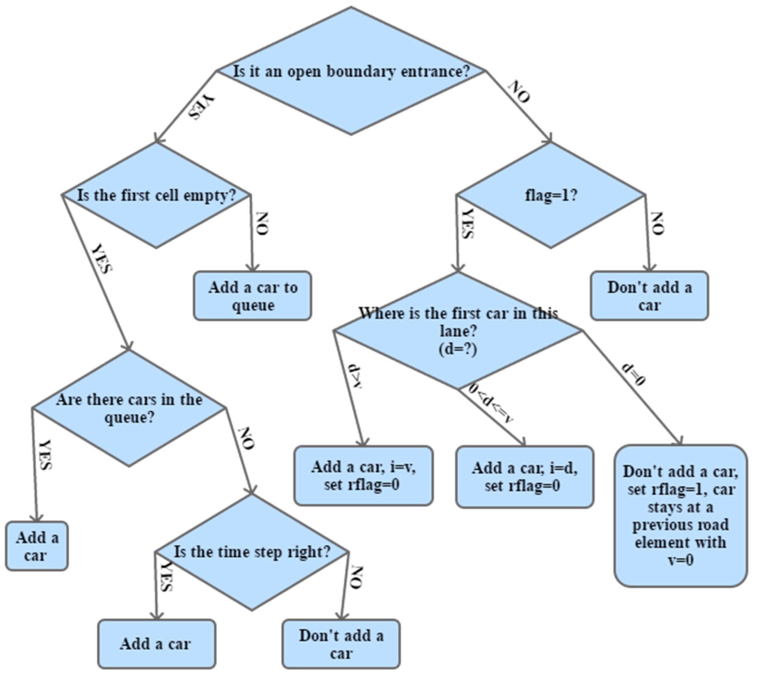
It is known that for computing logical operations in parallel, CPU is suited better than GPU, so the former route was chosen. The code is written using C/C++, and the MPI library is used for boundary condition exchange. Given the chosen parallelization method, though, it should be noted that data exchange requires additional steps. Basically, we have road elements that are calculated on different processors, and we need to exchange data when a car exits one element and enters another. However, if a traffic jam is formed in the target element, the car might not be able to enter it. In order to simulate this situation correctly, the boundary condition exchange algorithm has been created. It consists of two parts. The first one is shown in Figure 7 and it corresponds to vehicles’ entering a new element, from a different element/processor or entering the computational domain for the first time. If it is an open boundary entrance, the availability of the first cell is checked. If the cell is available, the car enters, if not, it is added to the queue, where it will wait till there is an unoccupied cell for it. If it’s an element in the middle of a road network, first thing the marker “flag” is checked, flag = 1 means that there is a vehicle that wants to enter.

If flag = 1, first several cells are checked for availability. If enough cells (according to vehicle’s speed) are empty, the vehicle is added. If possible, it can also be slowed down to fit in a new element. In these two cases, the data from the previous element is received and the car is added, and another marker, “rflag”, is set to 0 to indicate that the car has entered and should be deleted from the previous element. If the car cannot enter, rflag is set to 1, which means that the car stays in its element and waits for the opportunity to enter. When the opportunity presents itself, the message is sent to the other processor for this car to move.

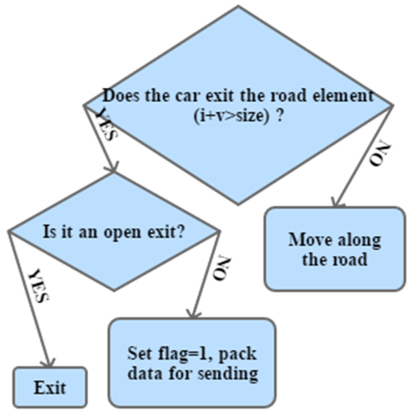
The second part of the algorithm is shown in Figure 8 and it corresponds to exiting an element.

When a car nears the boundary of the element and is ready to exit, the “flag” marker is set to 1 and is sent to the next element/processor, in case if there is one. If it is an open boundary, the car exits the computational domain.

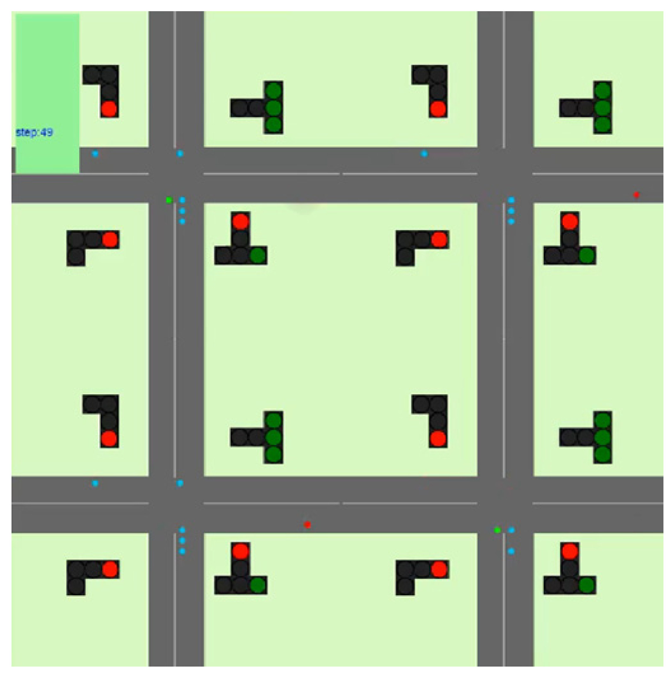
The example of a parallel computation on a small road network using the created model is shown in Figure 9.

The problem of the efficiency of the created parallel algorithm should be discussed. In order to be able to simulate traffic on various road networks, the set of universal road elements, such as signalized intersections, U-turns, road elements with widening/narrowing, etc., was created. From these elements, the desired network is formed before the computation, and each element is calculated using a single processor. This configuration allows forming numerous types of networks that can be found in cities, since the building blocks are universal, but it does not load the processors efficiently. For the efficient loading the elements should be much bigger, but this way they lose their flexibility in terms of creating any desired road configuration. This problem needs to be further investigated.

5. Discussion and Conclusions

Two original models created by the authors of this article and based on different approaches to traffic flow simulation are presented in this paper, and for each of them the parallel algorithm for numerical realization is discussed.

The new microscopic CA-based model is developed, using the CAM-2D model created earlier by the authors. The new model includes important algorithm changes regarding speed adaptation to fully comply with the three-phase theory, which is the requirement in the field nowadays. The parallel version of the calculation algorithm was developed using the domain decomposition technique. The special boundary condition exchange algorithm has been created to provide the correct transfer of data from one processor to another in case of congested traffic flow.

As a future direction of this work, for the CA approach, the parallelization efficiency increase is to be noted. Since the model possesses data parallelism, it might be promising to develop an algorithm using this quality in order to provide a sufficient load for computational nodes while still retaining the ability to form various road networks from single elements easily. Another important thing to do is a thorough verification and calibration process for the model using real experimental data.

The two-dimensional model of gas-dynamic type was presented. The model is based on the QGD system of equations. The difference from other macroscopic models is the presence of lateral velocity in the system of equations. The lateral velocity can be entered in various ways—in algebraic form or in differential form by analogy with forward velocity. The article presents both forms and concludes on the appropriateness of choosing of one way or another. The parallel version of the macroscopic simulation is based on the domain decomposition technique too.

The good scalability of the parallel algorithm for QGD traffic model was verified by numerical experiments evaluating strong scaling. The parallelization efficiency of about 80 percent on 100 CPU cores has been achieved which is fairly high efficiency for the class of problems under consideration. The obtained speedup is close to linear which is typical for algorithms based on explicit finite-difference schemes and domain decomposition. For the macroscopic QGD traffic model, the problem of increasing the parallelization efficiency is also relevant. In the current implementation on CPU cores, it would be efficient to calculate with a higher processor load, i.e., when modeling a larger urban network. The proposed macroscopic algorithm can also be implemented on GPUs. Creating a version of the algorithm for the hybrid architecture would enhance the universality of the code and its portability in a wide class of MPP systems.

The main achievement is that the developed approaches have internal parallelism. In particular, the proposed parallel algorithm facilitates the implementation of a 2D macroscopic model on the road network due to the exchange procedure at the nodes, thereby removing the problem of connecting road segments, which is present in the sequential implementation. It is important not only to speed up calculations, but also to get the correct implementation on the entire computational domain.

Parallel computations can provide a boost to the traffic flow modeling field, making computations on large-scale city road networks using modern and complex models not only possible, but rather fast as well. This topic of research has a great potential, as models and algorithms developed can be used as a part of ITS and be included in the “Smart City” concept.

The presented calculations were performed on supercomputers installed in the Centre of Collective Usage of KIAM RAS [41].

References

- Dimitrakopoulos, G.; Uden, L.; Varlamis, I. The Future of Intelligent Transport Systems, 1st ed.; Elsevier: Amsterdam, The Netherlands, 2020; 272p. [Google Scholar]
- Hamdar, S.; Talebpour, A.; Bertini, R. (Eds.) Traffic and Granular Flow. Spec. Issue J. Intell. Transp. Syst. 2020, 24, 535–653. [Google Scholar] [CrossRef]
- Ozbay, K.; Ban, X.; Yang, C.Y.D. (Eds.) Connected and Automated Vehicle-Highway Systems. Spec. Issue J. Intell. Transp. Syst. 2018, 22, 187–275. [Google Scholar] [CrossRef]
- Du, W.; Li, Y.; Zhang, J. Stability analysis and control of an extended car-following model under honk environment. Int. J. ITS Res. 2021. [Google Scholar] [CrossRef]
- Scharfe-Scherf, M.S.L.; Russwinkel, N. Familiarity and complexity during a takeover in highly automated driving. Int. J. ITS Res. 2021, 19, 525–538. [Google Scholar] [CrossRef]
- Guerrieri, M. Smart roads geometric design criteria and capacity estimation based on AV and CAV emerging technologies. A case study in the trans-European transport network. Int. J. ITS Res. 2021, 19, 429–440. [Google Scholar] [CrossRef]
- Chen, M.; Mao, S.; Zhang, Y.; Leung, V.C.M. Big Data. Related Technologies, Challenges and Future Prospects; Springer Briefs in Computer Science; Springer: Berlin/Heidelberg, Germany, 2014; 89p. [Google Scholar] [CrossRef]
- Treiber, M.; Kesting, A. Traffic Flow Dynamics. Data, Models and Simulation; Springer: Berlin/Heidelberg, Germany, 2013; pp. 55–238. [Google Scholar]
- Maerivoet, S.; De Moor, B. Cellular automata models of road traffic. Phys. Rep. 2005, 419, 1–64. [Google Scholar] [CrossRef] [Green Version]
- Sukhinova, A.B.; Trapeznikova, M.A.; Chetverushkin, B.N.; Churbanova, N.G. Two-dimensional macroscopic model of traffic flows. Math. Models Comput. Simul. 2009, 1, 669–676. [Google Scholar] [CrossRef]
- Trapeznikova, M.A.; Furmanov, I.R.; Churbanova, N.G.; Lipp, R. Simulating Multilane Traffic Flows Based on Cellular Automata Theory. Math. Models Comput. Simul. 2012, 4, 53–61. [Google Scholar] [CrossRef]
- Churbanova, N.G.; Chechina, A.A.; Trapeznikova, M.A.; Sokolov, P.A. Simulation of traffic flows on road segments using cellular automata theory and quasigasdynamic approach. Math. Montisnigri 2019, XLVI, 72–90. [Google Scholar] [CrossRef]
- Chetverushkin, B.N. Kinetic Schemes and Quasi-Gas Dynamic System of Equations; CIMNE: Barcelona, Spain, 2008; 298p. [Google Scholar]
- Nagel, K.; Schreckenberg, M. A cellular automaton model for freeway traffic. J. Phys. I France 1992, 2221–2229. [Google Scholar] [CrossRef]
- Chechina, A.; Churbanova, N.; Trapeznikova, M. Driver behaviour algorithms for the cellular automata-based mathematical model of traffic flows. EPJ Web Conf. 2021, 248, 02002. [Google Scholar] [CrossRef]
- Kerner, B.S.; Klenov, S.L.; Schreckenberg, M. Simple cellular automaton model for traffic breakdown, highway capacity, and synchronized flow. Phys. Rev. E 2011, 84, 046110. [Google Scholar] [CrossRef] [PubMed]
- Foster, I. Designing and Building Parallel Programs. Available online: http://www.mcs.anl.gov/~itf/dbpp/ (accessed on 29 December 2021).
- Lighthill, M.J.; Witham, G.B. On kinematic waves (Part II): A theory of traffic flow on long crowded roads. Proc. R. Soc. London Ser. A. Math. Phys. Sci. 1955, 229, 317–345. [Google Scholar] [CrossRef]
- Payne, H. Models of freeway traffic and control. In Mathematical Models of Public Systems; Bekey, G.A., Ed.; Simulation Council: La Jolla, CA, USA, 1971; Volume 3, pp. 51–61. [Google Scholar]
- Bando, M.; Hasebe, K.A.; Nakanishi, A.; Nakayama, A.; Shibata, Y.; Sugiyama, J. Phenomenological Study of Dynamical Model of Traffic Flow. J. Phys. I EDP Sci. 1995, 5, 1389–1399. [Google Scholar] [CrossRef] [Green Version]
- Newell, G.F. A simplified car-following theory: A lower order model. Transp. Res. Part B Methodol. 2002, 36, 195–205. [Google Scholar] [CrossRef]
- Phillips, W. A kinetic model for traffic flow with continuum implications. Transport. Plan. Technol. 1979, 5, 131–138. [Google Scholar] [CrossRef]
- Kuehne, R. Macroscopic freeway model for dense traffic–stop-start waves and incident detection. Transp. Traffic Theory 1984, 9, 20–42. [Google Scholar]
- Kerner, B.; Konhauser, P. Cluster effect in initially homogeneous traffic flow. Phys. Rev. E 1993, 48, 2335–2338. [Google Scholar] [CrossRef]
- Aw, A.; Rascle, M. Resurrection of “second order models” of traffic flow. SIAM J. Appl. Math. 2000, 60, 916–938. [Google Scholar]
- Zhou, J.; Zhang, H.L.; Wang, C.P.; Shi, Z.K. A new lattice model for single-lane traffic flow with the consideration of driver’s memory during a period of time. Int. J. Mod. Physics C 2017, 28, 1750086. [Google Scholar] [CrossRef]
- Jin, D.; Zhou, J.; Zhang, H.L.; Wang, C.P.; Shi, Z.K. Lattice hydrodynamic model for traffic flow on curved road with passing. Nonliear Dyn. 2017, 89, 107–124. [Google Scholar] [CrossRef]
- Kholodov, Y.A.; Alekseenko, A.E.; Vasil’ev, M.O.; Kholodov, A.S. Developing the mathematical model of road junction by the hydrodynamic approach. Comput. Res. Model. 2014, 6, 503–522. [Google Scholar] [CrossRef]
- Kaur, R.; Sharma, S. Analysis of driver’s characteristics on a curved road in lattice model. Phys. A Statstical Mech. Its Appl. 2017, 471, 59–67. [Google Scholar] [CrossRef]
- Cremer, M.; Ludwig, J. A fast simulation model for traffic flow on the basis of boolean operations. Math. Comput. Simul. 1986, 28, 297–303. [Google Scholar] [CrossRef]
- Larraga, M.E.; Alvarez-Icaza, L. Cellular automaton model for traffic flow based on safe driving policies and human reactions. Phys. A Stat. Mech. Its Appl. 2010, 389, 5425–5438. [Google Scholar] [CrossRef]
- Kerner, B.; Klenov, S.; Hermanns, G.; Schreckenberg, M. Effect of driver over-acceleration on traffic breakdown in three-phase cellular automaton traffic flow models. Phys. A Stat. Mech. Its Appl. 2013, 392, 4083–4105. [Google Scholar] [CrossRef]
- Jiang, H.; Zhang, Z.; Huang, Q.; Xie, P. Research of vehicle flow based on cellular automaton in different safety parameters. Saf. Sci. 2016, 82, 182–189. [Google Scholar] [CrossRef]
- Hou, G.; Chen, S. An improved cellular automaton model for work zone traffic simulation considering realistic driving behavior. J. Phys. Soc. Jpn. 2019, 88, 084001. [Google Scholar] [CrossRef]
- Top 500. The List. Available online: https://www.top500.org/ (accessed on 27 December 2021).
- Dongarra, J.J.; Luszczek, P.; Petitet, A. The LINPACK Benchmark: Past, present and future. Concurr. Computat. Pract. Exper. 2003, 15, 803–820. [Google Scholar] [CrossRef]
- Trapeznikova, M.A.; Churbanova, N.G.; Lyupa, A.A.; Morozov, D.N. Simulation of Multiphase Flows in the Subsurface on GPU-based Supercomputers. In Parallel Computing: Accelerating Computational Science and Engineering (CSE), Advances in Parallel Computing; IOS Press: Amsterdam, The Netherlands, 2014; Volume 25, pp. 324–333. [Google Scholar] [CrossRef]
- Kerner, B. The Physics of Traffic; Springer: Berlin/Heidelberg, Germany, 2004; 682p. [Google Scholar]
- Chechina, A.A.; Churbanova, N.G.; Trapeznikova, M.A. Comparison of reproduction of spatiotemporal structures of traffic flows using various ways of averaging data. Math. Models Comput. Simul. 2021, 13, 756–762. [Google Scholar] [CrossRef]
- Chechina, A.; Churbanova, N.; Trapeznikova, M.; Ermakov, A.; German, M. Traffic flow modelling on road networks using cellular automata theory. Int. J. Eng. Technol. 2018, 7, 225–227. [Google Scholar] [CrossRef]
- KIAM. The Official Site of Keldysh Institute of Applied Mathematics. Available online: https://www.kiam.ru/MVS/resourses/ (accessed on 28 December 2021).
Figure 1.
Decomposition of the computational domain into 12 sub-domains.
Figure 2.
Test problem geometry (a) and the spatiotemporal diagram of the effective density (b).
Figure 3.
Speedup in calculations of the problem about traffic on a highway with on-and off-ramps: (a) the initial code; and (b) the code with message passing optimization.
Figure 4.
Fragment of the Moscow map for traffic simulation.
Figure 5.
Effective density for two successive time moments for the road network near Chistoprudny Boulevard.
Figure 6.
Road fragment divided into cells.
Figure 7.
Boundary conditions exchange algorithm. Entrance.
Figure 8.
Boundary conditions exchange algorithm. Exit.
Figure 9.
Parallel computation on a road network.
Publisher’s Note: MDPI stays neutral with regard to jurisdictional claims in published maps and institutional affiliations. |
© 2022 by the authors. Licensee MDPI, Basel, Switzerland. This article is an open access article distributed under the terms and conditions of the Creative Commons Attribution (CC BY) license (https://creativecommons.org/licenses/by/4.0/).
Share and Cite
MDPI and ACS Style
Chetverushkin, B.; Chechina, A.; Churbanova, N.; Trapeznikova, M. Development of Parallel Algorithms for Intelligent Transportation Systems. Mathematics 2022, 10, 643. https://0-doi-org.brum.beds.ac.uk/10.3390/math10040643
AMA Style
Chetverushkin B, Chechina A, Churbanova N, Trapeznikova M. Development of Parallel Algorithms for Intelligent Transportation Systems. Mathematics. 2022; 10(4):643. https://0-doi-org.brum.beds.ac.uk/10.3390/math10040643
Chicago/Turabian StyleChetverushkin, Boris, Antonina Chechina, Natalia Churbanova, and Marina Trapeznikova. 2022. "Development of Parallel Algorithms for Intelligent Transportation Systems" Mathematics 10, no. 4: 643. https://0-doi-org.brum.beds.ac.uk/10.3390/math10040643
Note that from the first issue of 2016, this journal uses article numbers instead of page numbers. See further details here.