Analysis of Solutions, Asymptotic and Exact Profiles to an Eyring–Powell Fluid Modell

Abstract

The aim of this article was to provide analytical and numerical approaches to a one-dimensional Eyring–Powell flow. First of all, the regularity, existence, and uniqueness of the solutions were explored making use of a variational weak formulation. Then, the Eyring–Powell equation was transformed into the travelling wave domain, where analytical solutions were obtained supported by the geometric perturbation theory. Such analytical solutions were validated with a numerical exercise. The main finding reported is the existence of a particular travelling wave speed $a=1.212$ for which the analytical solution is close to the actual numerical solution with an accumulative error of <${10}^{-3}$.

1. Introduction

The Eyring–Powell flow is a type of non-Newtonian fluid of paramount relevance in industrial areas, manufacturing, and biological technology. Some trivial examples of non-Newtonian fluids are given by bubbles, boiling, plastic foam processing, columns, toothpaste, mud, honey, and custard. Non-Newtonian fluids are further classified into different classes by virtue of their rheological characteristic conditions. The Eyring–Powell fluid is one such subclass of non-Newtonian fluids with particular features linked with the kinetic theory of liquids. In their seminal paper, Metzner and Otto [1] considered a non-Newtonian fluid focused on the relationship between the speed of flow and shear rate. In 1982, Rajagopal [2] considered the incompressible, unidirectional, and unsteady conditions of a second-grade fluid to obtain solutions for a flow between two rigid plates in which one suddenly starts moving. Later on, with the help of Gupta [3], they established the exact solution for the same kind of fluid between porous plates. These cited seminal works have attracted the attention of the scientific community, leading to further research paths with the same topical background in non-Newtonian fluids. Eldabe et al. [4] obtained results applicable in the field of medicine and the study of blood flow, analysing the effect of coupling forces on an unstable non-Newtonian flow of MHD between two parallel fixed porous plates under a uniform external magnetic field. Another study, carried out by Shao and Lo [5], modelled the hydrodynamics of incompressible particles (SPHs) to simulate Newtonian and non-Newtonian flows with free surfaces. The authors were able to verify the proper functioning of the model in problems such as dam breaks in 2D. Another example of outstanding interest in this regard was the study carried out by Fetecau [6]. Here, solutions were established for unidirectional transient flows of non-Newtonian fluids in pipe-like domains.

Under particular rheological properties describing a non-Newtonian fluid, further applications have been accounted for by the theory of magnetohydrodynamics (MHD). Akbar [7] established the solution for a flow of a two-dimensional fluid under the effect of a magnetic field over stretching surfaces. Hina [8] analysed the heat transfer for the magnetohydrodynamic flow of the Eyring–Powell fluid. Later, Bhatti et al. [9] considered the same MHD fluid over permeable stretching surfaces. In this direction, other relevant studies can be considered (refer to [10,11,12,13,14,15]).

Further relevant topics in applied sciences involving Eyring–Powell fluids can be mentioned. In [16], the authors analysed the characteristics of the flow of Eyring–Powell nanofluids through a rotating disk subject to various physical phenomena such as a sliding flow and a magnetic field together with homogeneous and heterogeneous reactions. To this end, the proposed equations were solved by a numerical method based on the Runge–Kutta–Fehlberg method of 4th–5th order. Furthermore, in [17], the authors developed a computational technique for a three-dimensional Eyring–Powell fluid with activation energy on a stretched sheet with sliding effects. The resulting nonlinear system of PDEs was transformed into a nonlinear system of ODEs, and a shooting method was explored accordingly. The analysis in [18] discussed the flow and heat transfer of the Eyring–Powell MHD fluid in an infinite circular pipe. The explored solutions of different viscous terms were calculated numerically with the help of an iterative technique.

Note that in all the previously cited references, attention was mainly set on the numerical schemes in search of particular solutions. Analytical conceptions remain within the scope of dimensional analysis.

Further analytical approaches can be found in [19], where a homotopy approach was employed to construct solutions for a boundary layer with natural convection on a permeable vertical plate with thermal radiation. Afterwards, the differential quadrature method (DQM) was used to validate solutions for different parametrical cases involving the local Nusselt number and the local Sherwood number. In [20], the authors used the ADM-Padé approach to study analytical solutions for the deflection and pull-in instability of nanocantilever electromechanical switches, showing the remarkable accuracy compared with the numerical results. The authors claimed the possibility of extending their results to solve a wide range of instability problems. Furthermore, in [21], the authors studied a viscoelastic nanofluid with optimisation techniques subject to the proposal of a certain solution that was progressively optimised. To account for further analytical approaches, in [22], perturbation solutions were obtained for low-Reynolds–Eyring–Powell flow to obtain velocity, temperature, concentration, and stream functions.

After having cited some paramount studies involving analytical conceptions, it shall be noted that in the present study, the intention was to go deeper into the advances of the theory of PDEs to construct profiles of solutions. Unlike the previously cited studies, solutions were explored within the theory of travelling waves. Such a theory was firstly introduced by Kolmogorov, Petrovskii, and Piskunov [23], in combustion theory, and by Fisher [24], to predict the interaction of genes. The main question, introduced by the mentioned authors, was related to the search for an appropriate travelling wave speed for which the analytical travelling wave profile converges to the actual profile (solution of the actual problem, not converted into the travelling domain). Both the travelling profile and the actual one were shown to have the same exponential behaviour. This spirit was kept in our present analysis: indeed, one question to answer is related to the search for an appropriate travelling wave speed for which the analytically obtained solution converges to the actual one (obtained by numerical means) with a certain error tolerance. This was the main target of our analysis, but previously, the regularity, existence, and uniqueness of the solutions were shown. Later, the geometric perturbation theory was employed to support the construction of the analytical profiles of the solutions. These obtained profiles were validated afterwards via a numerical exercise.

2. Mathematical Model

We consider an incompressible, unsteady, and one-dimensional electrically conducting Eyring–Powell fluid. Under these assumptions, the velocity field is given by $\mathbf{V}=\left(u_1\left(y\right),0,0\right),$ where $u_1\left(y\right)$ refers to the first velocity component. Note that the proposed problem refers to an open geometry not shaped by dedicated containers or stretched by boundary conditions. The continuity and constitutive equations for an Eyring–Powell fluid are generally given by (refer to [25,26] for an additional discussion on the Eyring–Powell governing equations):

$$div\mathbf{V}=0,$$

(1)

and:

$${\rho }_f\frac{d\mathbf{V}}{dt}=div\mathbf{A}+\mathbf{J}\times \mathbf{B},$$

(2)

where ${\rho }_f$ refers to the density, $\mathbf{J}$ is the current density, $\mathbf{B}$ is the magnetic field, which can be split into $\mathbf{B}={\mathbf{B}}_0+\mathbf{b}$ where ${\mathbf{B}}_0$ and $\mathbf{b}$ are the imposed and induced magnetic fields, respectively, and $\mathbf{A}$ is given by:

$$\mathbf{A}=-p\mathbf{I}+{\tau }_{ij},$$

(3)

$$div\mathbf{B}=0,curl\mathbf{B}={\mu }_1\mathbf{j},curl\mathbf{E}=-\frac{\partial \mathbf{B}}{\partial t}$$

(4)

$$\mathbf{J}=\sigma \left(\mathbf{E}+\mathbf{V}\times \mathbf{B}\right),$$

(5)

where p is the pressure field, $\mathbf{I}$ is the identity tensor, ${\mu }_1$ is the magnetic permeability, $\mathbf{E}$ is the electric field, $\sigma$ is the electric conductivity, and ${\tau }_{ij}$ is the shear stress tensor of an Eyring–Powell fluid [11,13] given by:

$${\tau }_{ij}=\mu \frac{\partial u_i}{\partial x_j}+\frac{1}{\beta }{sinh}^{-1}\left(\frac{1}{d_1}\frac{\partial u_i}{\partial x_j}\right),$$

(6)

where $\mu$ is the dynamic viscosity and $\beta$ and $d_1$ are characteristic constants of the Powell-Eyring model. Consider that ${sinh}^{-1}\left(\frac{1}{d_1}\frac{\partial u_i}{\partial x_j}\right)\cong \frac{1}{d_1}\frac{\partial u_i}{\partial x_j}-\frac{1}{6}{\left(\frac{1}{d_1}\frac{\partial u_i}{\partial x_j}\right)}^3,$ $\left|\frac{1}{d_1}\frac{\partial u_i}{\partial x_j}\right|\le 1.$ The governing equation, in the absence of an induced magnetic field, can be written as:

$$\frac{\partial u_1}{\partial t}=-\frac{1}{\rho }\frac{dP}{dx}+\left(v+\frac{1}{\beta d_1{\rho }_f}\right)\frac{{\partial }^2{u}_1}{\partial y^2}-\frac{1}{2\beta d_1^3{\rho }_f}{\left(\frac{\partial u_1}{\partial y}\right)}^2\frac{{\partial }^2{u}_1}{\partial y^2}-\frac{\sigma B_0^2{u}_1}{{\rho }_f}.$$

(7)

where $v=\frac{\mu }{{\rho }_f}$ is the kinematic viscosity. After differentiation in (7) with x:

$$-\frac{1}{\rho }\frac{d^{2}P}{d{x}^2}=0,-\frac{1}{\rho }\frac{dP}{dx}=A_1.$$

Using the value of $-\frac{1}{\rho }\frac{dP}{dx}$ in (7), we obtain:

$$\frac{\partial u_1}{\partial t}=A_1+\left(v+\frac{1}{\beta d_1{\rho }_f}\right)\frac{{\partial }^2{u}_1}{\partial y^2}-\frac{1}{2\beta d_1^3{\rho }_f}{\left(\frac{\partial u_1}{\partial y}\right)}^2\frac{{\partial }^2{u}_1}{\partial y^2}-\frac{\sigma B_0^2{u}_1}{{\rho }_f}.$$

(8)

with the following initial condition:

$$u_1(y,0)=u_0\left(y\right)\in L_{loc}^1\left(R\right)\cap L^{\infty }\left(R\right).$$

(9)

3. Preliminaries

The proposed Eyring–Powell model in (8) is expressed making use of a weak formulation to support the analysis of the regularity, existence, and uniqueness of the solutions.

Definition 1. 

Consider a test function ${\varphi }_2\in C^{\infty }\left(R\right)$ defined in $(0,T)$, such that for $0<\tau <t<T$, the following weak formulation of (8) holds:

$$\begin{array}{c}\underset{R}{\int }{u}_1\left(t\right){\varphi }_2\left(t\right)dy=\underset{R}{\int }{u}_1\left(\tau \right){\varphi }_2\left(\tau \right)dy+\underset{\tau }{\overset{t}{\int }}\underset{R}{\int }{u}_1\frac{\partial {\varphi }_2}{\partial s}dyds\hfill \\ +A_1\underset{\tau }{\overset{t}{\int }}\underset{R}{\int }{\varphi }_{2}dyds+\left(v+\frac{1}{\beta d_1{\rho }_f}\right)\underset{\tau }{\overset{t}{\int }}\underset{R}{\int }{u}_1\frac{{\partial }^2{\varphi }_1}{\partial y^2}dyds\hfill \\ +\frac{1}{6\beta d_1^3{\rho }_f}\underset{\tau }{\overset{t}{\int }}\underset{R}{\int }{\left(\frac{\partial u_1}{\partial y}\right)}^3\frac{\partial {\varphi }_2}{\partial y}dyds-\frac{\sigma B_0^2}{{\rho }_f}\underset{\tau }{\overset{t}{\int }}\underset{R}{\int }{u}_1{\varphi }_{2}dyds.\hfill \end{array}$$

In addition, the following definition holds:

Definition 2. 

Given a finite spatial location $r_0$, admit a ball $B_r$ centred in $r_0$ and with radius $r\gg r_0$. In the proximity of the borders $\partial B_r$ and for $0<s<\tau <t<T$, the following equation is defined:

$$u_1\frac{\partial {\varphi }_2}{\partial s}+A_1{\varphi }_2+\left(v+\frac{1}{\beta d_1{\rho }_f}\right)u_1\frac{{\partial }^2{\varphi }_2}{\partial y^2}+\frac{1}{6\beta d_1^3{\rho }_f}{\left(\frac{\partial u}{\partial y}\right)}^3\frac{\partial {\varphi }_2}{\partial y}-\frac{\sigma B_0^2}{{\rho }_f}{u}_1{\varphi }_2=0,$$

(10)

in $B_r\times \left(0,T\right),$ with the following boundary and initial conditions:

$$0<\frac{\partial {\varphi }_2}{\partial y}={\varphi }_2\ll 1,$$

and:

$$u_1\left(y,0\right)=u_0\left(y\right)\in L_{loc}^1\left(R\right)\cap L^{\infty }\left(R\right).$$

4. Existence and Uniqueness Analysis

The following theorem aims to show the existence and bounds of the solutions:

Theorem 1. 

Given $u_0\left(y\right)\in L_{loc}^1\left(R\right)\cap L^{\infty }\left(R\right)$, then the solution is bounded for all $\left(y,t\right)\in B_r\times \left[\tau ,T\right)$ with $r\gg 1.$

Proof. 

Consider a certain value $\eta \in R^{+}$ such that the following cut-off function is defined (see [27,28]):

$${\psi }_{\eta }\in C_0^{\infty }\left(y,t\right),0\le {\psi }_{\eta }\le 1,$$

$${\psi }_{\eta }=1\mathrm{in}{B}_{r-\eta },{\psi }_{\eta }=0\mathrm{in}R-B_{r-\eta },$$

so that:

$$\left|\frac{\partial {\psi }_{\eta }}{\partial \eta }\right|=\frac{B_a}{\eta },$$

where $B_a$ is a suitable constant. Multiplying (10) by ${\psi }_{\eta }$ and integrating in $B_r\times \left[\tau ,T\right),$ we obtain:

$$\begin{gathered} \underset{\tau }{\overset{t}{\int }}\underset{B_r}{\int }{u}_1\frac{\partial {\varphi }_2}{\partial s}{\psi }_{\eta }dyds+A_1\underset{\tau }{\overset{t}{\int }}\underset{B_r}{\int }{\varphi }_2{\psi }_{\eta }dyds+\left(v+\frac{1}{\beta d_1{\rho }_f}\right)\underset{\tau }{\overset{t}{\int }}\underset{B_r}{\int }{u}_1\frac{{\partial }^2{\varphi }_2}{\partial y^2}{\psi }_{\eta }dyds \\ +\frac{1}{6\beta d_1^3{\rho }_f}\underset{\tau }{\overset{t}{\int }}\underset{B_r}{\int }{\left(\frac{\partial u_1}{\partial y}\right)}^3\frac{\partial {\varphi }_2}{\partial y}{\psi }_{\eta }dyds-\frac{\sigma B_0^2}{{\rho }_f}\underset{\tau }{\overset{t}{\int }}\underset{B_r}{\int }{u}_1{\varphi }_2{\psi }_{\eta }dyds=0. \end{gathered}$$

(11)

Now, admit an arbitrary $m>1$ and some large $r_0>1$ [27,28]:

$$\underset{\tau }{\overset{t}{\int }}{u}_{1}ds\le \underset{\tau }{\overset{t}{\int }}{u}_1^{m}ds\le D_1\left(\tau \right)r^{\frac{2m}{m-1}}.$$

Considering the spatial variable y close to $\partial B_r$, it can be assumed that $y\sim r$. Then, for $m=2,$ it holds that:

$$\underset{\tau }{\overset{t}{\int }}{u}_{1}ds\le D_1\left(\tau \right)r^4,\underset{\tau }{\overset{t}{\int }}{\left(\frac{\partial u_1}{\partial y}\right)}^{3}ds\le 64D_1^3\left(\tau \right)r^9.$$

The integral for the diffusion term reads:

$$\begin{array}{c}\left(v+\frac{1}{\beta d_1{\rho }_f}\right)\underset{\tau }{\overset{t}{\int }}\underset{B_r}{\int }{u}_1\frac{{\partial }^2{\varphi }_2}{\partial y^2}{\psi }_{\eta }dyds\hfill \\ \le \left(v+\frac{1}{\beta d_1{\rho }_f}\right)\underset{B_r}{\int }{D}_1\left(\tau \right)r^2\frac{{\partial }^2{\varphi }_2}{\partial y^2}{\psi }_{\eta }dy\hfill \\ =\left(v+\frac{1}{\beta d_1{\rho }_f}\right)D_1\left(\tau \right)r^2\left({\left(\frac{\partial {\varphi }_2}{\partial y}{\psi }_{\eta }\right)}_{\partial B_r}-\underset{B_r}{\int }\frac{\partial {\varphi }_2}{\partial y}\frac{\partial {\psi }_{\eta }}{\partial y}dy\right).\hfill \end{array}$$

As $r\gg 1$ and taking ${\varphi }_2$ sufficiently small such that $\frac{\partial {\varphi }_2}{\partial y}{\psi }_{\eta }\ll 1$ over $\partial B_r$, the following holds:

$$\begin{array}{c}\left(v+\frac{1}{\beta d_1{\rho }_f}\right)\underset{\tau }{\overset{t}{\int }}\underset{B_r}{\int }{u}_1\frac{{\partial }^2{\varphi }_2}{\partial y^2}{\psi }_{\eta }dyds\hfill \\ =-\left(v+\frac{1}{\beta d_1{\rho }_f}\right)\underset{B_r}{\int }{D}_1\left(\tau \right)r^2\frac{\partial {\varphi }_2}{\partial y}\frac{\partial {\psi }_{\eta }}{\partial y}dy\hfill \\ \le \left(v+\frac{1}{\beta d_1{\rho }_f}\right)D_1\left(\tau \right)\underset{B_r}{\int }{r}^2\frac{\partial {\varphi }_2}{\partial y}\frac{B_a}{\eta }dy\hfill \\ =\left(v+\frac{1}{\beta d_1{\rho }_f}\right)B_a{D}_1\left(\tau \right)\underset{B_r}{\int }r\frac{\partial {\varphi }_2}{\partial y}dy,\hfill \end{array}$$

and:

$$\frac{1}{6\beta d_1^3{\rho }_f}\underset{\tau }{\overset{t}{\int }}\underset{B_r}{\int }{\left(\frac{\partial u_1}{\partial y}\right)}^3\frac{\partial {\varphi }_2}{\partial y}{\psi }_{\eta }dyds\le \frac{32}{3\beta d_1^3{\rho }_f}\underset{B_r}{\int }{D}_1^3\left(\tau \right)r^9\frac{\partial {\varphi }_2}{\partial y}{\psi }_{\eta }dy.$$

Now:

$$\begin{array}{ccc}\hfill \frac{1}{6\beta d_1^3{\rho }_f}\underset{\tau }{\overset{t}{\int }}\underset{B_r}{\int }{\left(\frac{\partial u_1}{\partial y}\right)}^3\frac{\partial {\varphi }_2}{\partial y}{\psi }_{\eta }dyds& \le & -\frac{32}{3\beta d_1^3{\rho }_f}\underset{B_r}{\int }{D}_1^3\left(\tau \right)r^9{\varphi }_2\frac{\partial {\psi }_{\eta }}{\partial y}dy\hfill \\ & \le & \frac{32}{3\beta d_1^3{\rho }_f}\underset{B_r}{\int }{D}_1^3\left(\tau \right)r^9{\varphi }_2\frac{B_a}{\eta }dy\hfill \\ & =& \frac{32D_1^3\left(\tau \right)}{3\beta d_1^3{\rho }_f}\underset{B_r}{\int }{r}^8{\varphi }_{2}dy.\hfill \end{array}$$

(12)

Using the expressions (12) and (12) in (11), the following holds:

$$\begin{gathered} \underset{\tau }{\overset{t}{\int }}\underset{B_r}{\int }{u}_1\frac{\partial {\varphi }_2}{\partial s}{\psi }_{\eta }dyds+A_1\underset{\tau }{\overset{t}{\int }}\underset{B_r}{\int }{\varphi }_2{\psi }_{\eta }dyds\le \left(v+\frac{1}{\beta d_1{\rho }_f}\right)B_a{D}_1\left(\tau \right)\underset{B_r}{\int }r\frac{\partial {\varphi }_2}{\partial y}dy \\ +\frac{32B_a{D}_1^3\left(\tau \right)}{3\beta d_1^3{\rho }_f}\underset{B_r}{\int }{r}^8{\varphi }_{2}dy+\frac{\sigma B_0^2}{{\rho }_f}\underset{\tau }{\overset{t}{\int }}\underset{B_r}{\int }{u}_1{\varphi }_2{\psi }_{\eta }dyds. \end{gathered}$$

(13)

Next, consider a test function ${\varphi }_2$ of the form:

$${\varphi }_2\left(r,s\right)=e^{-ks}{\left(1+r^2\right)}^{-a}.$$

(14)

We can choose a in such a way that (13) is convergent; therefore:

$$\begin{array}{c}\left(v+\frac{1}{\beta d_1{\rho }_f}\right)B_a{B}_1\left(\tau \right)\underset{B_r}{\int }r\frac{\partial {\varphi }_2}{\partial y}dy+\hfill \\ \frac{32B_a{D}_1^3\left(\tau \right)}{3\beta d_1^3{\rho }_f}\underset{B_r}{\int }{r}^8{\varphi }_{2}dy+\frac{\sigma B_0^2{B}_1\left(\tau \right)}{{\rho }_f}\underset{B_r}{\int }{r}^2{\varphi }_2{\psi }_{\eta }dy\hfill \\ \le 2a\left(v+\frac{1}{\beta d_1{\rho }_f}\right)B_a{B}_1\left(\tau \right)\underset{B_r}{\int }{e}^{-ks}{r}^{-2a}dr\hfill \\ +\frac{32B_a{D}_1^3\left(\tau \right)}{3\beta d_1^3{\rho }_f}\underset{B_r}{\int }{r}^{8-2a}{\varphi }_{2}dr+\frac{\sigma B_0^2{B}_1\left(\tau \right)}{{\rho }_f}\underset{B_r}{\int }{e}^{-ks}{r}^{2-2a}dr.\hfill \end{array}$$

(15)

For $a>4$ and $r\to \infty ,$ the following holds:

$$\left(v+\frac{1}{\beta d_1{\rho }_f}\right)B_a{B}_1\left(\tau \right)\underset{B_r}{\int }r\frac{\partial {\varphi }_2}{\partial y}dy+\frac{\sigma B_0^2{B}_1\left(\tau \right)}{{\rho }_f}\underset{B_r}{\int }{r}^2{\varphi }_2{\psi }_{\eta }dy\le 0.$$

(16)

Putting (16) into (13):

$$\underset{\tau }{\overset{t}{\int }}\underset{B_r}{\int }{u}_1\frac{\partial {\varphi }_2}{\partial s}{\psi }_{\eta }dyds+A_1\underset{\tau }{\overset{t}{\int }}\underset{B_r}{\int }{\varphi }_2{\psi }_{\eta }dyds\le 0.$$

(17)

As both integrals are finite in $\tau <s<t<T,$ it is possible to conclude the theorem principles related to the bound of the solutions in $R\times (0,T).$ □

The next intention is to show the boundness of $\frac{\partial u_1}{\partial y}.$

Theorem 2. 

Given $u_1\left(y\right)$ as the solution of (8), then $\frac{\partial u_1}{\partial y}$ is bounded for $\left(y,t\right)\in R\times (0,T)$.

Proof. 

Multiplying the equation (8) by $u_1$ and using integration by parts:

$$\begin{array}{ccc}\hfill \frac{d}{dt}\underset{R}{\int }{\left|u_1\right|}^{2}dy& =& A_1\underset{R}{\int }{u}_{1}dy-\left(v+\frac{1}{\beta d_1{\rho }_f}\right)\underset{R}{\int }{\left(\frac{\partial u_1}{\partial y}\right)}^{2}dy\hfill \\ & & +\frac{1}{6\beta d_1^3{\rho }_f}\underset{R}{\int }{\left(\frac{\partial u_1}{\partial y}\right)}^{4}dy-\frac{\sigma B_0^2}{{\rho }_f}\underset{R}{\int }{\left|u_1\right|}^{2}dy,\hfill \end{array}$$

which implies that:

$$\begin{gathered} \underset{R}{\int }{\left(\frac{\partial u_1}{\partial y}\right)}^2\left(\frac{1}{6\beta d_1^3{\rho }_f}{\left(\frac{\partial u_1}{\partial y}\right)}^2-\left(v+\frac{1}{\beta d_1{\rho }_f}\right)\right)dy=\frac{d}{dt}\underset{R}{\int }{\left|u_1\right|}^{2}dy \\ -A_1\underset{R}{\int }{u}_{1}dy-\frac{\sigma B_0^2}{{\rho }_f}\underset{R}{\int }{\left|u_1\right|}^{2}dy. \end{gathered}$$

After integration on both sides:

$$\begin{gathered} \underset{0}{\overset{t}{\int }}\underset{R}{\int }{\left(\frac{\partial u_1}{\partial y}\right)}^2\left(\frac{1}{6\beta d_1^3{\rho }_f}{\left(\frac{\partial u_1}{\partial y}\right)}^2-\left(v+\frac{1}{\beta d_1{\rho }_f}\right)\right)dyds=\underset{R}{\int }{\left|u_1(y,t)\right|}^{2}dy \\ -\underset{R}{\int }{\left|u_0\left(y\right)\right|}^{2}dy-A_1\underset{0}{\overset{t}{\int }}\underset{R}{\int }{u}_{1}dyds-\frac{\sigma B_0^2}{{\rho }_f}\underset{0}{\overset{t}{\int }}\underset{R}{\int }{\left|u_1\right|}^{2}dyds. \end{gathered}$$

(18)

From Theorem (1), the right-hand side of (18) is bounded; therefore, we can choose $A_2$ such that:

$$\underset{0}{\overset{t}{\int }}\underset{R}{\int }{\left(\frac{\partial u_1}{\partial y}\right)}^2\left(\frac{1}{6\beta d_1^3{\rho }_f}{\left(\frac{\partial u_1}{\partial y}\right)}^2-\left(v+\frac{1}{\beta d_1{\rho }_f}\right)\right)dyds\le A_2,$$

(19)

which permits concluding that $\frac{\partial u_1}{\partial y}$ is bounded in $R\times (0,t)$ where we can admit $t=T$. □

The next intention is to show the uniqueness of the solution.

Theorem 3. 

Let us admit $u_1>0$ as a minimal solution and ${\widehat{u}}_1$ as a maximal solution for (8) in $R\times (0,T)$, then $u_1$ coincides with the maximal solution ${\widehat{u}}_1$, i.e., the solution is unique.

Proof. 

Consider ${\widehat{u}}_1$ to be the maximal solution of (8) in $R\times (0,T)$ given by:

$${\widehat{u}}_1\left(y,0\right)=u_0\left(y\right)+ϵ,$$

(20)

with $ϵ>0$ arbitrarily small. In addition, let us define the minimal solution:

$$u_1\left(y,0\right)=u_0\left(y\right).$$

The maximal and minimal solutions satisfy the following equations:

$$\begin{array}{ccc}\hfill \frac{\partial {\widehat{u}}_1}{\partial t}& =& A_1+\left(v+\frac{1}{\beta d_1{\rho }_f}\right)\frac{{\partial }^2{\widehat{u}}_1}{\partial y^2}-\frac{1}{2\beta d_1^3{\rho }_f}{\left(\frac{\partial {\widehat{u}}_1}{\partial y}\right)}^2\frac{{\partial }^2{\widehat{u}}_1}{\partial y^2}-\frac{\sigma B_0^2{\widehat{u}}_1}{{\rho }_f},\hfill \end{array}$$

(21)

$$\begin{array}{ccc}\hfill \frac{\partial u_1}{\partial t}& =& A_1+\left(v+\frac{1}{\beta d_1{\rho }_f}\right)\frac{{\partial }^2{u}_1}{\partial y^2}-\frac{1}{2\beta d_1^3{\rho }_f}{\left(\frac{\partial u_1}{\partial y}\right)}^2\frac{{\partial }^2{u}_1}{\partial y^2}-\frac{\sigma B_0^2{u}_1}{{\rho }_f}.\hfill \end{array}$$

(22)

For every test function ${\varphi }_2\in C^{\infty }\left(R\right)$ and upon subtraction, the following expressions hold:

$$\begin{array}{cc}\hfill 0& \le \underset{R}{\int }\left({\widehat{u}}_1-u_1\right){\varphi }_2\left(t\right)dy=\underset{0}{\overset{t}{\int }}\underset{R}{\int }\left({\widehat{u}}_1-u_1\right)\frac{\partial {\varphi }_2}{\partial s}dyds\hfill \\ & +\left(v+\frac{1}{\beta d_1{\rho }_f}\right)\underset{0}{\overset{t}{\int }}\underset{R}{\int }\left({\widehat{u}}_1-u_1\right)\frac{{\partial }^2{\varphi }_2}{\partial y^2}dyds\hfill \\ \hfill & +\frac{1}{6\beta d_1^3{\rho }_f}\underset{0}{\overset{t}{\int }}\underset{R}{\int }\left({\left(\frac{\partial {\widehat{u}}_1}{\partial y}\right)}^3-{\left(\frac{\partial u_1}{\partial y}\right)}^3\right)\frac{{\partial }^2{\varphi }_2}{\partial y^2}dyds-\frac{\sigma B_0^2}{{\rho }_f}\underset{0}{\overset{t}{\int }}\underset{R}{\int }\left({\widehat{u}}_1-u_1\right)\varphi dyds\hfill \\ \hfill & \le \underset{0}{\overset{t}{\int }}\underset{R}{\int }\left({\widehat{u}}_1-u_1\right)\frac{\partial {\varphi }_2}{\partial s}dyds+\left(v+\frac{1}{\beta d_1{\rho }_f}\right)\underset{0}{\overset{t}{\int }}\underset{R}{\int }\left({\widehat{u}}_1-u_1\right)\frac{{\partial }^2{\varphi }_2}{\partial y^2}dyds\hfill \\ \hfill & +\frac{1}{6\beta d_1^3{\rho }_f}\underset{0}{\overset{t}{\int }}\underset{R}{\int }\left(\frac{\partial {\widehat{u}}_1}{\partial y}-\frac{\partial u_1}{\partial y}\right)\left({\left(\frac{\partial {\widehat{u}}_1}{\partial y}\right)}^2+\frac{\partial {\widehat{u}}_1}{\partial y}\frac{\partial u_1}{\partial y}+{\left(\frac{\partial u_1}{\partial y}\right)}^2\right)\frac{\partial {\varphi }_2}{\partial y}dyds\hfill \\ \hfill & -\frac{\sigma B_0^2}{{\rho }_f}\underset{0}{\overset{t}{\int }}\underset{R}{\int }\left({\widehat{u}}_1-u_1\right)\varphi dyds\hfill \end{array}$$

(23)

Based on Theorem 2’s results, we can choose $A_3$ such that $A_3=sup\{\frac{\partial {\widehat{u}}_1}{\partial y},\frac{\partial u_1}{\partial y}\}$, so that the following holds:

$$\begin{gathered} \underset{R}{\int }\left({\widehat{u}}_1-u_1\right){\varphi }_2\left(t\right)dy\le \underset{0}{\overset{t}{\int }}\underset{R}{\int }\left({\widehat{u}}_1-u_1\right)\frac{\partial {\varphi }_2}{\partial s}dyds+\left(v+\frac{1}{\beta d_1{\rho }_f}\right)\underset{0}{\overset{t}{\int }}\underset{R}{\int }\left({\widehat{u}}_1-u_1\right)\frac{{\partial }^2{\varphi }_2}{\partial y^2}dyds \\ +\frac{A_3}{6\beta d_1^3{\rho }_f}\underset{0}{\overset{t}{\int }}\underset{R}{\int }\left(\frac{\partial {\widehat{u}}_1}{\partial y}-\frac{\partial u_1}{\partial y}\right)\frac{\partial {\varphi }_2}{\partial y}dyds-\frac{\sigma B_0^2}{{\rho }_f}\underset{0}{\overset{t}{\int }}\underset{R}{\int }\left({\widehat{u}}_1-u_1\right)\varphi dyds \\ =\underset{0}{\overset{t}{\int }}\underset{R}{\int }\left(\widehat{u_1}-u_1\right)\frac{\partial {\varphi }_2}{\partial s}dyds+\left(v+\frac{1}{\beta d_1{\rho }_f}-\frac{A_3}{6\beta d_1^3{\rho }_f}\right)\underset{0}{\overset{t}{\int }}\underset{R}{\int }\left(\widehat{u_1}-u_1\right)\frac{{\partial }^2{\varphi }_2}{\partial y^2}dyds \end{gathered}$$

(24)

$$-\frac{\sigma B_0^2}{{\rho }_f}\underset{0}{\overset{t}{\int }}\underset{R}{\int }\left({\widehat{u}}_1-u_1\right)\varphi dyds.$$

(25)

Now, consider the test function given by:

$${\varphi }_2\left(\left|y\right|,s\right)=e^{A_4\left(T-s\right)}{\left(1+{\left|y\right|}^2\right)}^{-b},$$

(26)

where $A_4$ and b are constants. Making the differentiation of ${\varphi }_2$ with regards to s and $y,$ the following holds:

$$\frac{\partial {\varphi }_2}{\partial s}=-A_4{\varphi }_2\left(\left|y\right|,s\right),\frac{{\partial }^2{\varphi }_2}{\partial y^2}\le A_5\left(b\right){\varphi }_2\left(\left|y\right|,s\right),$$

then:

$$\left({\widehat{u}}_1-u_1\right)\frac{\partial {\varphi }_2}{\partial s}+\left(v+\frac{1}{\beta d_1{\rho }_f}-\frac{A_3}{6\beta d_1^3{\rho }_f}\right)\left({\widehat{u}}_1-u_1\right)\frac{{\partial }^2{\varphi }_2}{\partial y^2}-\frac{\sigma B_0^2}{{\rho }_f}\left({\widehat{u}}_1-u_1\right){\varphi }_2$$

$$\begin{array}{ccc}\hfill & \le & -A_4{\varphi }_2\left({\widehat{u}}_1-u_1\right)+\left(v+\frac{1}{\beta d_1{\rho }_f}-\frac{A_3}{6\beta d_1^3{\rho }_f}\right)A_5\left(b\right){\varphi }_2\left({\widehat{u}}_1-u_1\right)-\frac{\sigma B_0^2}{{\rho }_f}\left({\widehat{u}}_1-u_1\right){\varphi }_2\hfill \\ & =& \left(-A_4+\left(v+\frac{1}{\beta d_1{\rho }_f}-\frac{A_3}{6\beta d_1^3{\rho }_f}\right)A_5\left(b\right)-\frac{\sigma B_0^2}{{\rho }_f}\right)\left({\widehat{u}}_1-u_1\right){\varphi }_2.\hfill \end{array}$$

(27)

Using (27) in (24), we obtain:

$$\begin{array}{c}\underset{R}{\int }\left({\widehat{u}}_1-u_1\right){\varphi }_2\left(t\right)dy\le \left(-A_4+\left(v+\frac{1}{\beta d_1{\rho }_f}-\frac{A_3}{6\beta d_1^3{\rho }_f}\right)A_5\left(b\right)-\frac{\sigma B_0^2}{{\rho }_f}\right)\hfill \\ \times \underset{0}{\overset{t}{\int }}\underset{R}{\int }\left({\widehat{u}}_1-u_1\right){\varphi }_{2}dyds\le \left|-A_4+\left(v+\frac{1}{\beta d_1{\rho }_f}-\frac{A_3}{6\beta d_1^3{\rho }_f}\right)A_5\left(b\right)-\frac{\sigma B_0^2}{{\rho }_f}\right|\hfill \\ \times \underset{0}{\overset{t}{\int }}\underset{R}{\int }\left({\widehat{u}}_1-u_1\right){\varphi }_{2}dyds.\hfill \end{array}$$

(28)

Making the differentiation with regard to t:

$$\begin{array}{c}\frac{d}{dt}\underset{R}{\int }\left({\widehat{u}}_1-u_1\right){\varphi }_2\left(t\right)dy\le \left|-A_4+\left(v+\frac{1}{\beta d_1{\rho }_f}-\frac{A_3}{6\beta d_1^3{\rho }_f}\right)A_5\left(b\right)-\frac{\sigma B_0^2}{{\rho }_f}\right|\hfill \\ \times \underset{R}{\int }\left({\widehat{u}}_1-u_1\right){\varphi }_2\left(t\right)dy.\hfill \end{array}$$

(29)

Now, let us define:

$$h\left(t\right)=\underset{R}{\int }\left({\widehat{u}}_1-u_1\right){\varphi }_2\left(t\right)dy.$$

(30)

Putting (30) into (29), the following holds:

$$\frac{dh}{dt}\le \left|-A_4+\left(v+\frac{1}{\beta d_1{\rho }_f}-\frac{A_3}{6\beta d_1^3{\rho }_f}\right)A_5\left(b\right)-\frac{\sigma B_0^2}{{\rho }_f}\right|h\left(t\right),$$

(31)

with:

$$h\left(0\right)=ϵ\to 0.$$

After solving (31) by standard means, we obtain $h\left(t\right)=0,$ i.e., ${\widehat{u}}_1=u_1,$ which shows the uniqueness of the solutions, as was intended to be proven. □

5. Travelling Waves’ Existence and Regularity

The travelling wave profiles are described as $u_1\left(y,t\right)=k\left(\zeta \right)$, where $\zeta =y-at\in R,$ a refers to the travelling wave speed and $k:R\to \left(0,\infty \right)$ belongs to $L^{\infty }\left(R\right).$

The equation (8) is transformed into the travelling wave domain as follows:

$$-a{k}^{\prime }\left(\zeta \right)=A_1+\left(v+\frac{1}{\beta d_1{\rho }_f}\right)k^{″}\left(\zeta \right)-\frac{1}{2\beta d_1^3{\rho }_f}{\left(k^{\prime }\left(\zeta \right)\right)}^2{k}^{″}\left(\zeta \right)-\frac{\sigma B_0^2}{{\rho }_f}k\left(\zeta \right).$$

(32)

with $k^{\prime }\left(\zeta \right)<0$ in the hypothesis of a purely decreasing travelling wave (this assumption is further discussed later). Now, let us consider the following new variables:

$$X=k\left(\zeta \right),Y=k^{\prime }\left(\zeta \right),$$

(33)

such that the following system holds:

$$\begin{array}{ccc}\hfill X^{\prime }& =& Y,\hfill \\ \hfill Y^{\prime }& =& \frac{2\beta d_1^3{\rho }_f}{2v\beta d_1^3{\rho }_f+2d_1^2-Y^2}\left(-aY-A_1+\frac{\sigma B_0^2}{{\rho }_f}X\right).\hfill \end{array}$$

(34)

To analyse the suggested system in the proximity of the critical point, admit $X^{\prime }=0$ and $Y^{\prime }=0$, yielding:

$$X=\frac{A_1{\rho }_f}{\sigma B_0^2}.$$

Therefore, $\left(\frac{A_1{\rho }_f}{\sigma B_0^2},0\right)$ represents the system critical point.

Our intention in the coming sections was to make use of the geometric perturbation theory to characterise the existing critical point and to explore solution orbits close to such a critical point.

5.1. Geometric Perturbation Theory

In this section, we use the singular geometric perturbation theory to show the asymptotic behaviour of an appropriately defined manifold close to the critical point. Afterwards, the obtained results are used to derive a dedicated travelling wave profile.

For this purpose, admit the following manifold as:

$$N_0=\left\{X,Y/X^{\prime }=Y;Y^{\prime }=\frac{2\beta d_1^3{\rho }_f}{2v\beta d_1^3{\rho }_f+2d_1^2-Y^2}\left(-aY-A_1+\frac{\sigma B_0^2}{{\rho }_f}X\right)\right\},$$

(35)

with critical point $\left(\frac{A_1{\rho }_f}{\sigma B_0^2},0\right).$ The perturbed manifold $N_{ϵ}$ close to $N_0$ in the critical point $\left(\frac{A_1{\rho }_f}{\sigma B_0^2},0\right)$ is defined as:

$$N_{ϵ}=\left\{X,Y/X^{\prime }=ϵY;Y^{\prime }=Fϵ\left(X-\frac{A_1{\rho }_f}{\sigma B_0^2}\right)\right\},$$

(36)

where $ϵ$ denotes a perturbation parameter close to equilibrium $\left(X_1,0\right)$ and F is a suitable constant, which is found after root factorisation. Firstly, admit $X_3=X-\frac{A_1{\rho }_f}{\sigma B_0^2}$. Our intention was to apply the Fenichel invariant manifold theorem [29] as formulated in [30]. For this purpose, we have to show that $N_0$ is a normally hyperbolic manifold, i.e., the eigenvalues of $N_0$ in the linearised frame close to the critical point, and transversal to the tangent space, have non-zero real part. This is shown based on the following equivalent flow associated with $N_0:$

$$\left(\genfrac{}{}{0pt}{}{X_3^{\prime }}{Y^{\prime }}\right)=\left(\begin{array}{cc}0& ϵ\\ Fϵ& 0\end{array}\right)\left(\genfrac{}{}{0pt}{}{X_3}{Y}\right).$$

The associated eigenvalues are both real $\left(\pm \sqrt{F}ϵ\right),$ which shows that $N_0$ is a hyperbolic manifold. Now, we want to show that the manifold $N_{ϵ}$ is locally invariant under the flow (34), so that the manifold $N_0$ can be shown as an asymptotic approach to $N_{ϵ}$ and vice versa. On this basis, we consider the functions:

$$\begin{array}{ccc}\hfill {\psi }_1& =& ϵY,\hfill \\ \hfill {\psi }_2& =& FϵX_3,\hfill \end{array}$$

which are $C^i\left(R\times \left[0,\delta \right)\right)$, $i>0$, in the proximity of the critical point $\left(\frac{A_1{\rho }_f}{\sigma B_0^2},0\right).$ In this case, $\delta$ is determined based on the following flows that are considered to be measurable a.e. in $R:$

$$∥{\psi }_1^{M_0}-{\psi }_1^{M_{ϵ}}∥\le Fϵ∥X_3∥\le \delta ϵ.$$

Since the solutions are bounded, we conclude that $\delta =F∥X_3∥$ is finite; therefore, the distance between the manifolds holds the normal hyperbolic condition for $\delta \in \left(0,\infty \right)$ and $ϵ$ sufficiently small close to the critical point $\left(\frac{A_1{\rho }_f}{\sigma B_0^2},0\right)$.

5.2. Travelling Waves’ Profiles

Based on the normal hyperbolic condition shown for the manifold $N_0$ under the flow (34), asymptotic TW profiles can be obtained. For this purpose, let us consider firstly (34) such that the following family of trajectories in the phase plane $\left(X,Y\right)$ holds:

$$\frac{dY}{dX}=\frac{2\beta d_1^3{\rho }_f}{\left(2v\beta d_1^3{\rho }_f+2d_1^2-Y^2\right)Y}\left(-aY-A_1+\frac{\sigma B_0^2}{{\rho }_f}X\right)=H\left(X,Y\right).$$

(37)

As $H\left(X,Y\right)$ is continuous and is changing the sign character if we take X sufficiently large and sufficiently small, it is possible to conclude the existence of a critical trajectory of the form:

$$-a{X}^{\prime }-A_1+\frac{\sigma B_0^2}{{\rho }_f}X=0,$$

which implies that:

$$X^{\prime }=\frac{\sigma B_0^2}{a{\rho }_f}\left(X-\frac{A_1{\rho }_f}{\sigma B_0^2}\right).$$

(38)

Solving (38), we obtain:

$$X=\frac{A_1{\rho }_f}{\sigma B_0^2}+e^{\frac{\sigma B_0^2}{a{\rho }_f}\zeta }.$$

After using the value of $X,$ we obtain:

$$k\left(\zeta \right)=\frac{A_1{\rho }_f}{\sigma B_0^2}+e^{\frac{\sigma B_0^2}{a{\rho }_f}\zeta },$$

which implies that:

$$u_1\left(y,t\right)=\frac{A_1{\rho }_f}{\sigma B_0^2}+e^{\frac{\sigma B_0^2}{a{\rho }_f}\left(y-at\right)}.$$

This last expression shows the existence of an exponential profile along the travelling wave frame. This is not a trivial result for the nonlinear reaction under the Eyring–Powell fluid.

Note that the solution holds by the symmetry $(\zeta \to -\zeta )$ of travelling wave profiles. It suffices to admit $\zeta =y+at$, so that:

$$k\left(\zeta \right)=\frac{A_1{\rho }_f}{\sigma B_0^2}+e^{-\frac{\sigma B_0^2}{a{\rho }_f}\zeta },u_1\left(y,t\right)=\frac{A_1{\rho }_f}{\sigma B_0^2}+e^{-\frac{\sigma B_0^2}{a{\rho }_f}\left(y+at\right)}.$$

(39)

Now, it is the aim to show that the defined supporting manifold $N_{ϵ}$ preserves the exponential behaviour close to the critical points. For this purpose, the expression (36) is re-written as:

$$\frac{dY}{dX}=\frac{F}{Y}\left(X-\frac{A_1{\rho }_f}{\sigma B_0^2}\right).$$

(40)

After solving (40):

$$Y=F\left(X-\frac{A_1{\rho }_f}{\sigma B_0^2}\right).$$

(41)

From the expression (36), the equation (41) becomes:

$$X^{\prime }=Fϵ\left(X-\frac{A_1{\rho }_f}{\sigma B_0^2}\right).$$

(42)

After solving (42), we have:

$$X=\frac{A_1{\rho }_f}{\sigma B_0^2}+e^{Fϵ\zeta }.$$

(43)

From (33), the expression (43) becomes:

$$k\left(\zeta \right)=\frac{A_1{\rho }_f}{\sigma B_0^2}+e^{Fϵ\zeta },u_1\left(y,t\right)=\frac{A_1{\rho }_f}{\sigma B_0^2}+e^{Fϵ\left(y-at\right)}.$$

This last expression permits showing the conservation of the exponential profile close to the critical points defined by the asymptotic manifolds $N_{ϵ}.$

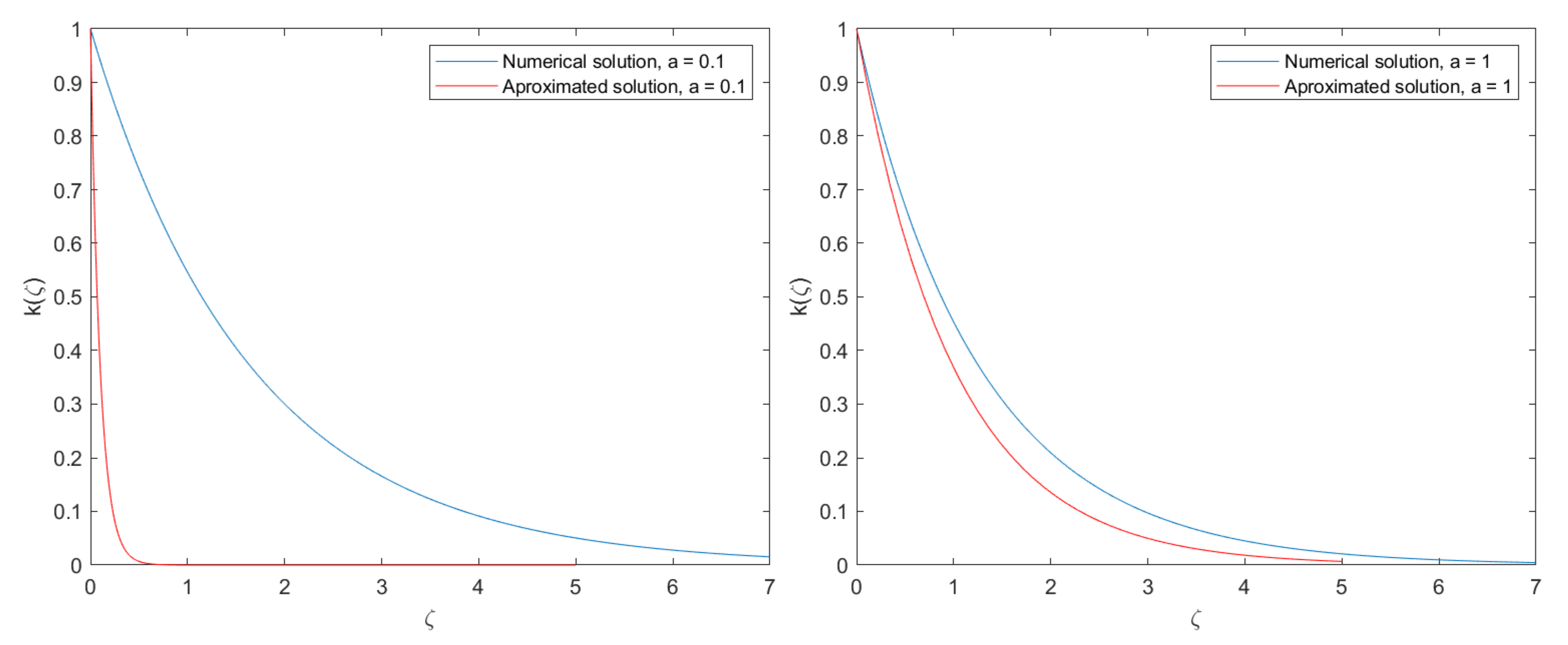
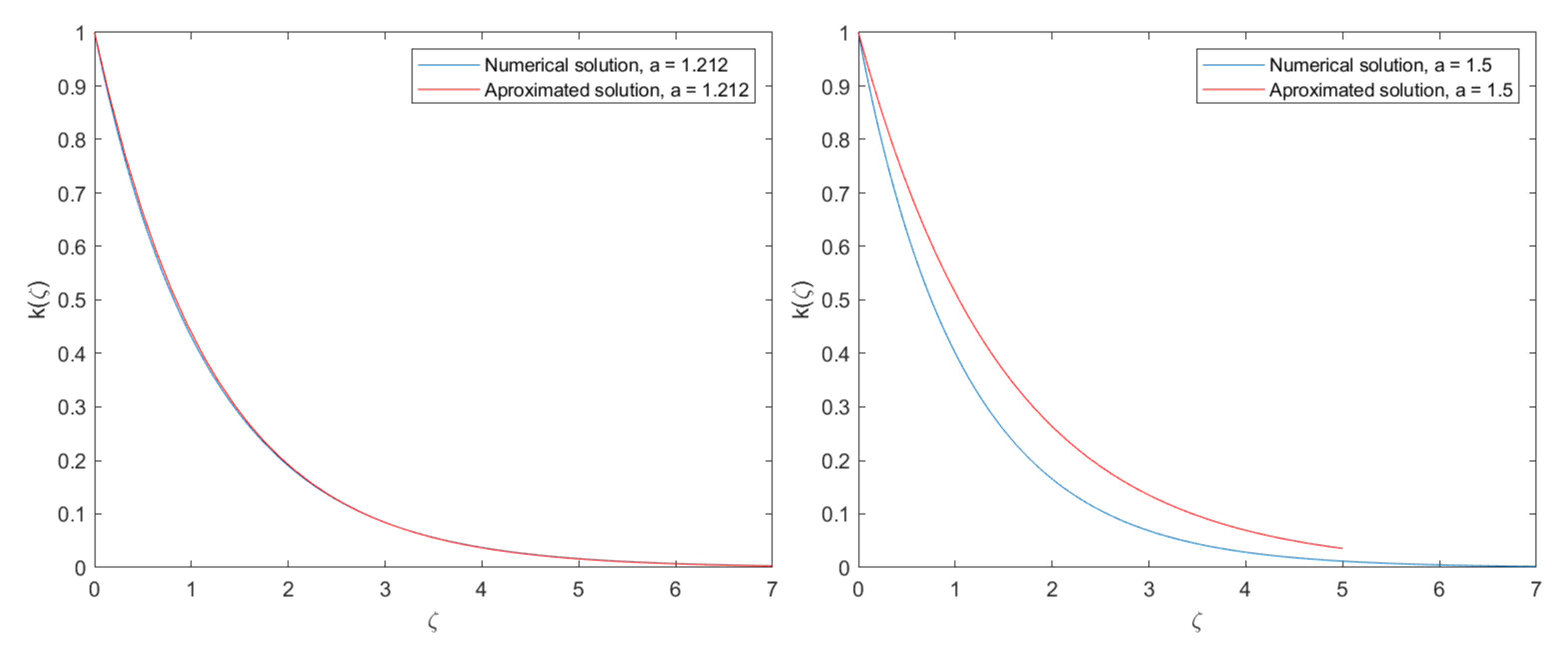
6. Numerical Validation Assessments

The aim in this section is to develop a numerical simulation to determine an appropriate travelling wave velocity (a) for which the approximated analytical solution (39) and the exact one, obtained numerically, in (34) behave similarly. This exercise can be seen as a validation process of the obtained analytical paths presented in the previous sections. This validation was explored for certain combinations of the fluid properties. Note that other combinations do not have an impact on the analytical ending in the exponential kind of solutions.

The numerical exploration was performed as per the following principles:

• The solver bvp4c in MATLAB was employed. This solver is based on a Runge–Kutta implicit approach with interpolant extensions [31]. The bvp4c collocation method requires specifying pseudo-boundary conditions. In this case, the left boundary is considered positive, $k(\zeta \to -\infty )=1$, and the right boundary is given by the null critical state, $k(\zeta \to \infty )=0$. As the intention was to determine the exact coincidence along the profiles for which the exponential tail is given, the solutions were translated into the zero state by the standard vertical translation;
• The integration domain was assumed as $(-200,200)$, sufficiently large so as to hinder any potential effect of the pseudo-boundary conditions imposed by the collocation method involved in the bvp4c solver;
• The domain was split into 100,000 nodes with an absolute error of ${10}^{-5}$ during the computation;
• An absolute error criterion was considered to stop the exploration criteria. The travelling wave speed for which both solutions, the numerically exact one and the analytical approach, were sufficiently close with an absolute error of $<{10}^{-3}$, named as the critical $a^{*}$. For this particular speed, The analytical solution in (39) can be regarded as a valid solution to the problem (34);
• The associated fluid constants in (34) were as one. The travelling wave speed a was the parameter used in the search for an analytical profile matching the error tolerance. In addition and with no loss of generality, $A_1=0$. Note that this particular selection of constant values did not impact the ending conclusions, i.e., on the existence of an analytical exponential profile matching the exact solution for a certain value in the travelling wave speed.

The results are compiled in Figure 1, Figure 2 and Figure 3. The existence of a critical travelling wave speed $a^{*}=1.212$ for which the analytical solution in (39) is close to the numerically exact one of (34) with an accumulative error of <${10}^{-3}$ was concluded. This numerical exploration permits accounting for the validation of the analytical exponential profile obtained.

7. Conclusions

The presented analysis in this article permitted accounting for the regularity, existence, and uniqueness of solutions to an Eyring–Powell fluid flow. Solutions were explored in the travelling wave domain, and asymptotic approaches were provided making use of the singular geometric perturbation theory. Afterwards, the obtained analytical solution was validated for a certain combination of fluid constants and making use of a numerical exercise. The existence of a travelling wave speed of $a=1.212$ for which the analytical solution is close to the actual numerical solution with an accumulative error of <${10}^{-3}$ was concluded. The existence of an exponential travelling wave tail together with a certain minimizing error critical speed constituted the main novelty reported by the present study.

References

1. Metzner, A.; Otto, R. Agitation of non-Newtonian fluids. AIChE J. 1957, 3, 3–10. [Google Scholar] [CrossRef]
2. Rajagopal, K. A note on unsteady unidirectional flows of a non-Newtonian fluid. Int. J. Non Linear Mech. 1982, 17, 369–373. [Google Scholar] [CrossRef]
3. Rajagopal, K.; Gupta, A. An exact solution for the flow of a nonNewtonian fluid past an infinite porous plate. Meccanica 1984, 19, 158–160. [Google Scholar] [CrossRef]
4. Eldabe, N.; Hassan, A.; Mohamed, M.A. Effect of couple stresses on the MHD of a non-Newtonian unsteady flow between two parallel porous plates. Z. Naturforschung A 2003, 58, 204–210. [Google Scholar] [CrossRef] [Green Version]
5. Shao, S.; Lo, E.Y. Incompressible SPH method for simulating Newtonian and non-Newtonian flows with a free surface. Adv. Water Resour. 2003, 26, 787–800. [Google Scholar] [CrossRef]
6. Fetecau, C. Analytical solutions for non-Newtonian fluid flows in pipe-like domains. Int. J. Non-Linear Mech. 2004, 39, 225–231. [Google Scholar] [CrossRef]
7. Akbar, N.S.; Ebaid, A.; Khan, Z. Numerical analysis of magnetic field effects on Eyring–Powell fluid flow towards a stretching sheet. J. Magn. Magn. Mater. 2015, 382, 355–358. [Google Scholar] [CrossRef]
8. Hina, S. MHD peristaltic transport of Eyring–Powell fluid with heat/mass transfer, wall properties and slip conditions. J. Magnetism. Magn. Mater. 2016, 404, 148–158. [Google Scholar] [CrossRef]
9. Bhatti, M.; Abbas, T.; Rashidi, M.; Ali, M.; Yang, Z. Entropy generation on MHD Eyring–Powell nanofluid through a permeable stretching surface. Entropy 2016, 18, 224. [Google Scholar] [CrossRef] [Green Version]
10. Ara, A.; Khan, N.A.; Khan, H.; Sultan, F. Radiation effect on boundary layer flow of an Eyring–Powell fluid over an exponentially shrinking sheet. Ain Shams Eng. J. 2004, 5, 1337–1342. [Google Scholar] [CrossRef] [Green Version]
11. Hayat, T.; Iqbal, Z.; Qasim, M.; Obaidat, S. Steady flow of an Eyring–Powell fluid over a moving surface with convective boundary conditions. Int. J. Heat Mass Transfer. 2012, 55, 1817–1822. [Google Scholar] [CrossRef]
12. Hayat, T.; Awais, M.; Asghar, S. Radiactive effects in a three dimensional flow of MHD Eyring–Powell fluid. J. Egypt Math. Soc. 2013, 21, 379–384. [Google Scholar] [CrossRef] [Green Version]
13. Jalil, M.; Asghar, S.; Imran, S.M. Self similar solutions for the flow and heat transfer of Powell-Eyring fluid over a moving surface in parallel free stream. Int. J. Heat Mass Transf. 2013, 65, 73–79. [Google Scholar] [CrossRef]
14. Khan, J.A.; Mustafa, M.; Hayat, T.; Farooq, M.A.; Alsaedi, A.; Liao, S.J. On model for three-dimensional flow of nanofluid: An application to solar energy. J. Mol. Liq. 2014, 194, 41–47. [Google Scholar] [CrossRef]
15. Riaz, A.; Ellahi, R.; Sait, S.M. Role of hybrid nanoparticles in thermal performance of peristaltic flow of Eyring–Powell fluid model. J. Therm. Anal. Calorim. 2021, 143, 1021–1035. [Google Scholar] [CrossRef]
16. Gholinia, M.; Hosseinzadeh, K.; Mehrzadi, H.; Ganji, D.D.; Ranjbar, A.A. Investigation of MHD Eyring–Powell fluid flow over a rotating disk under effect of homogeneous–heterogeneous reactions. Case Stud. Therm. Eng. 2019, 13, 100356. [Google Scholar] [CrossRef]
17. Umar, M.; Akhtar, R.; Sabir, Z.; Wahab, H.A.; Zhiyu, Z.; Imran, A.; Shoaib, M.; Raja, M.A.Z. Numerical treatment for the three-dimensional Eyring–Powell fluid flow over a stretching sheet with velocity slip and activation energy. Adv. Math. Phys. 2019, 2019, 9860471. [Google Scholar] [CrossRef] [Green Version]
18. Nazeer, M.; Ahmad, F.; Saeed, M.; Saleem, A.; Naveed, S.; Akram, Z. Numerical solution for flow of a Eyring–Powell fluid in a pipe with prescribed surface temperature. J. Braz. Soc. Mech. Sci. Eng. 2019, 41, 1–10. [Google Scholar] [CrossRef]
19. Talebizadeh, P.; Moghimi, M.A.; Kimiaeifar, A.; Ameri, M. Numerical and analytical solutions for natural convection flow with thermal radiation and mass transfer past a moving vertical porous plate by DQM and HAM. Int. J. Comput. Methods 2011, 8, 611–631. [Google Scholar] [CrossRef]
20. Noghrehabadi, A.; Ghalambaz, M.; Ghanbarzadeh, A. A new approach to the electrostatic pull-in instability of nanocantilever actuators using the ADM–Padé technique. Comput. Math. Appl. 2012, 64, 2806–2815. [Google Scholar] [CrossRef] [Green Version]
21. Noghrehabadi, A.; Mirzaei, R.; Ghalambaz, M.; Chamkha, A.; Ghanbarzadeh, A. Boundary layer flow heat and mass transfer study of Sakiadis flow of viscoelastic nanofluids using hybrid neural network-particle swarm optimization (HNNPSO). Therm. Sci. Eng. Prog. 2017, 4, 150–159. [Google Scholar] [CrossRef]
22. Hayat, T.; Tanveer, A.; Yasmin, H.; Alsaadi, F. Simultaneous effects of Hall current and thermal deposition in peristaltic transport of Eyring–Powell fluid. Int. J. Biomath. 2015, 8, 1550024. [Google Scholar] [CrossRef]
23. Kolmogorov, A.N.; Petrovskii, I.G.; Piskunov, N.S. Study of the diffusion equation with growth of the quantity of matter and its application to a biological problem. Byull. Moskov. Gos. Univ. 1937, 1, 1–25. [Google Scholar]
24. Fisher, R.A. The advance of advantageous genes. Ann. Eugen. 1937, 7, 355–369. [Google Scholar] [CrossRef] [Green Version]
25. Bilal, M.; Ashbar, S. Flow and heat transfer analysis of Eyring–Powell fluid over stratified sheet with mixed convection. J. Egypt. Math. Soc. 2020, 28, 40. [Google Scholar] [CrossRef]
26. Ramzan, M.; Bilal, M.; Kanwal, S.; Chung, J.D. Effects of variable thermal conductivity and nonlinear thermal radiation past an Eyring–Powell nanofluid flow with chemical reaction. Commun. Theor. Phys. 2017, 67, 723–731. [Google Scholar] [CrossRef]
27. Pablo, A.D. Estudio de una Ecuación de Reacción—Difusión. Ph.D. Thesis, Universidad Autónoma de Madrid, Madrid, Spain, 1989. [Google Scholar]
28. Pablo, A.D.; Vázquez, J.L. Travelling waves and finite propagation in a reaction–diffusion Equation. J Differ. Equ. 1991, 93, 19–61. [Google Scholar] [CrossRef] [Green Version]
29. Fenichel, N. Persistence and smoothness of invariant manifolds for flows. Indiana Univ. Math. J. 1971, 21, 193–226. [Google Scholar] [CrossRef]
30. Jones, C.K.R. Geometric Singular Perturbation Theory in Dynamical Systems; Springer: Berlin/Heidelberg, Germany, 1995. [Google Scholar]
31. Enright, H.; Muir, P.H. A Runge-Kutta Type Boundary Value ODE Solver with Defect Control; Teh. Rep. 267/93; University of Toronto, Dept. of Computer Sciences: Toronto, ON, Canada, 1993. [Google Scholar]
Figure 1. a = 0.1 (left), a = 1 (right). The blue line is the exact numerical profile of the set of Equations (34). The red line is the analytical solution obtained in (39) up to ζ = 5 (beyond such values, it is required to change the scale). Solutions on the left are provided for a = 1 and solutions on the right for a = 1.5 . For increasing values of the travelling speed, the solutions behave similarly in their exponential tail.
Mathematics 10 00660 g001
Figure 2. a = 1.212 (left), a = 1.5 (right). The blue line is the exact numerical profile of the set of Equations (34). The red line is the analytical solution obtained in (39). The approximated solution and the exact profile closely match an accumulative error (as the integration of the difference of both solutions) of < 10 3 for a = 1.212 . Solutions on the right are given for a = 1.5 . The approximated solution is above the numerical one.
Mathematics 10 00660 g002
Figure 3. a = 2 (left), a = 3 (right). The blue line is the exact numerical profile of the set of Equations (34). The red line is the analytical solution obtained in (39). Solutions on the left are provided for a = 2 and solutions on the right for a = 3 . Note that for increasing values of the travelling wave speed, both profiles diverge.
Mathematics 10 00660 g003
Publisher’s Note: MDPI stays neutral with regard to jurisdictional claims in published maps and institutional affiliations.