
Balancing the Electromagnetic Field Exposure in Wireless Multi-Hop Networks: An EMF-Aware Routing Scheme


1
Computer Science and Engineering Department, University Politehnica of Bucharest, Splaiul Independenţei nr.313, 060042 Bucharest, Romania
2
Communications Engineering Department, Universidad de Cantabria, Avda. Los Castros, s/n, 39005 Santander, Spain
*
Author to whom correspondence should be addressed.
Mathematics 2022, 10(4), 668; https://0-doi-org.brum.beds.ac.uk/10.3390/math10040668
Submission received: 14 January 2022
/
Revised: 8 February 2022
/
Accepted: 16 February 2022
/
Published: 21 February 2022
(This article belongs to the Special Issue Automatic Control and Soft Computing in Engineering)
Abstract
:This work is situated at the conjunction of the fields of distributed systems, telecommunications, and mathematical modeling, aiming to offer solutions to the problem of people’s overexposure to electro-magnetic fields (EMF) radiation. In this paper, we propose a new routing scheme for wireless multi-hop networks, which seeks a fairer distribution of the exposure to electromagnetic fields, by leveraging a combination of the transmitted power and the accumulated exposure as a routing metric. We carry out a holistic approach, including: (1) an algorithmic study, (2) an analytical model of the aforementioned novel routing metric, and (3) the specification of a routing protocol. We make a performance assessment of our novel routing protocol and the corresponding algorithm, by means of an extensive simulation campaign over the NS-3 simulator. The obtained results yield that the proposed novel solution is able to not only fairly distribute the exposure, but also to reduce its average value, thus enhancing the user experience. We also show that the power consumption using the EMF-aware proposed solution, based on Cycle Canceling Algorithm (CCA), and that observed with an approach seeking power reduction are alike. Indeed, even if there exist key-differences from the user experience’s point of view between both routing approaches, there is no statistically relevant power increase between them. Thus, our solution manages to keep the consumed power at a low level, and at the same time it reduces the overall nodes’ exposure to EMF.
1. Introduction
In recent years we have witnessed an unprecedented increase in the use of wireless communications. Furthermore, it is expected that the overall Internet traffic will double between 2018 and 2023 [1], and the number of connected devices per person will grow from to during the same period. Although it is almost impossible to envisage our day-to-day life without the use of smart-phones or tablets, there is also an increasing concern about the negative effects that the exposure to electromagnetic fields (EMF) may have on the general population, which has led the International Comission on Non-ionizing Radiation Protection (ICNIRP) to fix new limits to EMF in 2020 [2]. In this regard, the leitmotiv of the Low EMF Exposure Networks (LEXNET) [3] European project was to tackle this challenge, by advocating the use of different management techniques and novel communication technologies to reduce the EMF exposure induced by wireless communication systems, without jeopardizing the quality of experience perceived by end-users. However, the adoption of new wireless technologies and frequency bands under the 5G umbrella, such as Millimeter Waves (mmWave), is leading the scientific community to re-address the effects of EMF [4], while authorities are fostering such research initiatives. In this sense, the European Commission has recently launched a call on this topic with a budget of EUR 40 million (call Environment and health (2021) (HORIZON-HLTH-2021-ENVHLTH-02)).
Among the communication alternatives that have received more attention from the scientific community, this work deals with wireless multi-hop topologies. Although their origins date back to 1997 (with the IETF MANET working group), the traditional application scenarios that were proposed at that time have significantly changed, moving from war and natural disaster circumstances, to use-cases focused on expanding the coverage of base stations in a simple and economical way. It is worth noting, for example, the relevance of such deployments within the increasingly widespread wireless sensor networks, and the role given to them in the new specifications of the 5G technology, i.e., relaying techniques and Device-to-Device communications [5].
The routing mechanisms that have been traditionally used over wireless multi-hop networks foster the selection of minimum-cost paths, in many cases seeking those alternatives with the least number of hops. In this work, however, we propose to penalize paths exhibiting a higher EMF exposure. Unlike the number of hops, the EMF exposure is not directly related to the Quality of Service (QoS), but to the population’s health and, to their perception when using the communication services. In this regard, using the EMF exposure as a quality indicator to develop new communication solutions and to improve existing ones would have a positive impact on the user Quality of Experience (Quality of Experience). Keeping this in mind, the Exposure Index (EI) was defined under the umbrella of the LEXNET project as a metric to quantify the population exposure to the EMF induced by communication systems. This metric combines parameters related to the wireless technologies (i.e., frequency bands), with life segmentation information (i.e., time of the day, technology usages, etc.) to provide an overall estimation of the exposure, as defined in Equation (1). In particular, it is defined as a temporal average, over a period T, of the exposure induced by different combinations of technology-related parameters and segmentation data. We refer to each combination as an exposure component, while corresponds to the number of considered components.
The LEXNET EI takes into account, for every component, the number of devices, , and, for each device, the uplink transmitted power, (in W) as well as the downlink incident power density, (W/m2). Other parameters, shown in Equation (1), are used to weigh each component’s contribution, and the contribution brought by uplink/downlink communications. The reader may refer to [6] for a more detailed description of the LEXNET EI.
The LEXNET EI is related to the Specific Absortion Rate (SAR) (the same measurement unit as well: W/Kg), which is a parameter defined for mobile devices that is strongly correlated with the accumulated power involved in wireless transmissions. Since the goal is to propose a routing protocol that can be used over real networks, the routing metrics that will be exploited are to serve as proxies for the overall EI. The assumption is that, if the proposed scheme is able to optimize some of these proxy parameters, among which the most important is the transmit power, from which the accumulated power is directly derived, it would also lead to an eventual reduction of the overall EI.
To the best of our knowledge, when it comes to routing in multi-hop decentralized networks, even if the EMF accumulated exposure (such as the LEXNET EI), or other related parameter, has been used to optimize the physical and media access layer of deployed networks, it has not yet been taken into consideration as a routing metric, this being one of the key original contributions of this paper. This is a novel metric, defined within [6], where the EMF EI is defined as the summation of the entire SAR over a particular area, and over all people within such an area. Even if the LEXNET EI, which we also use as metric in this paper, highly depends of the transmit power of each node, it is not identical to this, especially due to its accumulated nature. In our work we indeed use the instant transmit power as a proxy for the more complicated EI metric, whenever this was appropriate, but in the end our routing decision at each node’s level is taken with respect to the entire accumulated exposure of each node, that is, the sum of all the transmit powers that the node had to use at various previous moments in time. This way, besides minimizing the induced nodes’ exposure, the algorithm and protocol that we have designed and implemented also leverage a load balancing of the decentralized distributed system, namely it does not over-stress a popular route and thus does not create EMF hotspots. We achieve this avoidance of EMF hotspots by gradually increasing costs for any route, when the exposure of the involved nodes becomes too high. This yields a changing network topology, since some graph edges from the initial multi-hop network may be un-usable after having been used too intensively, thus favoring less popular routes.
In our work, we were more interested in the network and node behavior as theoretical models, rather on the particular details of a technique to route the packets between the nodes. This is why we have chosen, as the underlying routing protocol, the well-known Ad hoc On-Demand Distance Vector Routing (AODV) [7], modified to solve the minimum cost flow problem that arises from minimizing the exposure, as we will describe in the following sections. In particular, we adopt the Cycle Canceling Algorithm (CCA) algorithm to solve the corresponding optimization problem. The integration of CCA into the AODV operation leads to the so-called EMF Aware AODV (EA-AODV). On top of the routing protocol and algorithm, we have used techniques similar to peer-to-peer relay networks, in order to minimize each node’s exposure, as defined in the LEXNET EI.
Before designing the routing protocol, we formulate an optimization problem and propose an algorithm based on graph theory to solve it. This will establish the performance baseline for the routing protocol. In particular, by adding virtual nodes, the network model does not only account for static metrics, but also for both the cumulative characteristic of the EMF exposure, and for the dynamic network. The optimum paths are finally obtained by means of a modified version of the CCA solution.
Afterwards, we strictly define the proxies for the EI that will be used to assess the performance of the proposed protocol. The operation of EA-AODV relies on the theoretical models of the aforementioned EI proxies. Its performance is studied by means of an extensive simulation campaign carried out over the NS-3 framework, where we compare EA-AODV to more traditional approaches. Throughout the analysis, we assume that nodes can dynamically adapt their transmission power, based on the characteristics of the links they have with their corresponding neighbors.
Altogether, this work makes the following contributions:
- Definition of a general exposure model for wireless multi-hop networks;
- Introduction of an optimization problem to include the EMF exposure in routing schemes;
- Proposal of a novel EMF-aware routing protocol based on AODV, coined EA-AODV, that practically solves the aforementioned optimization problem;
- Implementation of EA-AODV protocol in the NS-3 framework;
- Evaluation of the EA-AODV operation in comparison with legacy solutions.
The paper is structured as follows. Section 2 discusses some related works, and places the contributions that are presented herewith in the state of the art context. Then, Section 3 presents our proposal for EMF-aware routing scheme. To this end, it first depicts the corresponding optimization problem, introducing an algorithm that uses graph theory to solve it. Afterwards, an analytical model for EMF exposure in wireless multi-hop networks is presented. This model is then used to define the operation of the EA-AODV protocol. Then, in Section 4 we assess the exposure model presented before and analyze the performance of the proposed solution, comparing it with legacy approaches. Finally, Section 5 concludes the paper, outlining possible future research directions.
2. Related Work
As discussed in Section 1, we have witnessed, in recent years, an upturn on the research regarding multi-hop topologies. Their original purpose, as emergency scenarios, has led to other innovative applications and use cases. Nowadays, either Wireless Sensor Networks (WSN) or device-to-device (D2D) communications can have a significant impact on the individual exposure of humans, due to the body proximity of the involved devices.
Indeed, routing in WSN is still actively investigated for different application use cases related to 5G and beyond 5G. For instance, in [8] the authors propose a novel ad-hoc routing protocol, so-called VARP, specially designed to enhance the performance of 5G wireless networks leveraging D2D capabilities. In addition, depending on the specific targets and scenarios, different methods are applied to solve the routing problem. In this sense, Pattnaik et al. [9] applied genetic algorithms to select the best routing from a set of them in Mobile Ad-hoc Networks (MANET) scenarios, exploiting the On-demand Multipath Distance Vector (AOMDV). Following a different approach, fuzzy Petri nets and ant colony optimization techniques are used in [10] to improve the QoS parameters, such as delivery ratio, throughput, or delay.
Similar to the number of methods, the range of application use cases is also very broad. In this regard, the authors of [11] study routing for D2D communications using mmWave technology. Another routing solution in a MANET scenario is presented in [12], as part of a mobile edge computing setup embracing drones. In particular, this work combines data forwarding and task offloading. Similarly, Wang et al. apply in [13] routing over a Vehicular Ad-hoc Netorks (VANET) scenario for intelligent transportation systems, as a key service vertical addressed by 5G communication technology. The authors propose a protocol named low-latency and energy efficient routing based on network connectivity (LENC), which is able to outperform legacy solutions. As can be observed from the literature review, routing in multi-hop wireless networks is still a key technique for present and forthcoming use cases.
As for routing metrics, they have traditionally focused on QoS parameters, such as delay, hop count, or power [14,15]. Based on these parameters, the routing metrics can be divided into two main categories [16]: (1) single-radio, and (2) multi-radio. From the single-radio category, the Expected Transmission Count (ETX) [17] and the Expected Transmission Time (ETT) [18] are two of the most widespread alternatives, and they have been enhanced and broadened with the Weighted Cummulative Expected Transmission Time (WCETT) [18], the Exclusive Expected Transmission Time (EETT) [19], or with other solutions that take into consideration the interference phenomenon. The Metric for Interference and Channel Switching (MIC) [20] or the Interference Aware (iAWARE) [21] are examples belonging to the multi-radio category. Somehow related to EMF exposure, Green Networking gathered the attention from the scientific community. The main idea behind it is promoting an energy-aware behavior, mostly by means of reducing the transmitted power, increasing at the same time the battery life-time. Most of the existing proposals [22,23] deal with cellular communications, while not much attention has been paid to wireless multi-hop topologies. As of today, novel solutions pursue optimizing the same performance parameters, but energy, alone or combined with other criteria, is becoming more relevant. In this regard, Veeraiah et al. propose in [24] a routing technique to trade off energy efficiency and security. Similarly, a joint optimization problem, accounting for power control and routing, is posed and solved, using Benders decomposition, in [25]. The authors focus on the performance of the analytical solution, rather than addressing it from a protocol perspective. Slightly different to other works, the authors of [26] extend routing to drones, leading to the so called flying ad-hoc network (FANET), again paying attention to energy consumption.
However, only a few works have specifically used EMF exposure, or other related parameters as a routing parameter in the past. One of them is the one presented in [27]. In this work, the authors introduce a band selection scheme for D2D, where Nearest Neighbor Routing (NRR) is used as the routing solution. Nevertheless, this work differs from ours in various aspects. First, it does not propose a routing solution, but it exploits an existing one (NRR) and provides a band-selection scheme. In addition, the work presented in [27] addresses the routing problem from a theoretical perspective. On the other hand, we provide a whole framework for EMF routing, ranging from the metrics definition to a concrete protocol implementation.
Based on a newly minted routing metric that considers the EMF exposure, in this work we define and evaluate a novel routing protocol, which is an extension of the ones described in [28,29], where preliminary ideas and partial implementations were presented. Regarding legacy routing solutions, two main approaches exist for multi-hop wireless networks: (1) reactive, in which nodes trigger route discovery procedures only when they need to; and (2) proactive, where nodes periodically send topology-related information, which is afterwards used to establish the corresponding routes. One of the main advantages of the reactive protocols is that, especially for moderate traffic loads, they exhibit a better energy consumption behavior. Hence, since the main goal of this work is to reduce the exposure, the core functionality of one the most widespread reactive protocols, AODV [7], was exploited to develop the solution proposed herewith.
The effect sought by the novel protocol is twofold: (1) a reduction of the overall exposure, closely related to the transmitted power; (2) the aim to avoid EMF hot-spots, thus copying the behavior of load-balancing solutions. The reader might refer to the survey by Rathan et al. [30] for a succinct discussion of the most interesting load balancing proposals.
3. EMF-Aware Routing Framework for WMNs
In this section we present several components defined to address the EMF exposure in Wireless Mesh Networks (WMNs). First, we present a theoretical framework to consider the exposure on a WMN in Section 3.1. Then we describe the algorithm defined for EMF-aware routing, and the protocol that implements it in Section 3.2 and Section 3.3, respectively.
3.1. Theoretical Approach of EMF Exposure on WMNs
We first introduce a mathematical function that could be used to characterize the EMF exposure in a WMN. This will be afterwards used to identify performance indicators to be used in the EMF-aware routing protocol for this type of networks. In a nutshell, we consider the EMF in wireless networks as a cumulative effect that is induced in an area surrounding a transmitter. This way, the higher the transmission power and number of times a node transmits, the higher the exposure. In this work we will not take into account other effects such as antenna directionality, which may have a strong impact on the induced exposure, but we focus on the routing networking techniques.
3.1.1. General Description of the Exposure Model
We consider a WMN of N nodes and define as a vector with the exposure induced by all nodes at a particular moment of time t. From the routing point of view, the exposure grows every time a node sends or forwards a packet and remains constant in those moments in which the node is idle. We will use the transmission power required to send a packet as a proxy metric for the exposure. Furthermore, we assume that nodes are able to dynamically adapt their transmission power. It seems sensible to state that the growth rate of the exposure induced by a node, when transmitting a packet, can be expressed as a function of its transmission power. Hence, the exposure proxy can also be seen as the slope (first derivative) of the exposure, and which without the loss of generality is defined as a function () of the transmission power, , as defined in Equation (2).
A reduction of the slope of this per node accumulated exposure function, would actually yield a smaller exposure. For instance, it would be beneficial to always establish the minimum power for transmitting or forwarding, i.e., selecting the next hop according to the power required to reach it. On the other hand, it would also be interesting studying how the accumulated exposure pace varies along the time. This can be matched to the second derivative, , of the accumulated exposure at each individual node.
3.1.2. Computing the Exposure on WMNs
Let us focus on the accumulated exposure induced by a particular node k up to time t (), and let us assume that both the first and second derivative functions (, respectively) exist. Under these hypotheses we can establish the following properties:
- 1.
- Since the exposure is accumulative, ;
- 2.
- Consequently, , corresponding to this growing function over t;
- 3.
- Depending on the value of , we can establish various circumstances, as can be seen below:
- If , the rhythm of accumulating exposure on node k is increasing;
- If , the pace of accumulating exposure on node k is constant;
- If , the rhythm of accumulating exposure on node k is decreasing.
Based on these three properties, we can find an appropriate proxy for the exposure, which can be used as a means to design EMF-aware routing mechanisms over multi-hop wireless networks. We assume, without loss of generality, that time is slotted. We do not impose any limitation on the number of packets transmitted within one slot. Hence, the exposure induced by node k will increase between two consecutive time slots, provided it transmits any packet in-between; otherwise it will remain constant. In addition, the pace at which increases depends on both the number of transmitted packets and the transmission power required for the node k’s packet to reach its destination. Based on these observations, Theorem 1 defines the exposure for continuous time.
Theorem 1.
The exposure induced by node k in t can be calculated as follows
where and are known constants. The proof is given in Appendix A.
Since we have assumed that time is discretized, we can express the double integral in Theorem 1 by summing the values of in the various slots, yielding Theorem 2.
Theorem 2.
Assuming that the exposure induced by node k is zero at slot 0, we can express the exposure induced by node k at slot n as follows:
The proof is given in Appendix B.
3.1.3. Integrating the EMF Exposure into Routing
According to the previous definitions, the exposure induced by a node grows according to how it sends packets. It is worth highlighting that the theoretical model is not constrained by the power used to send each packet, but it only considers the event of sending. Depending on the technology, as well as on the power used to reach the next hop within the route, the accumulated exposure will grow differently.
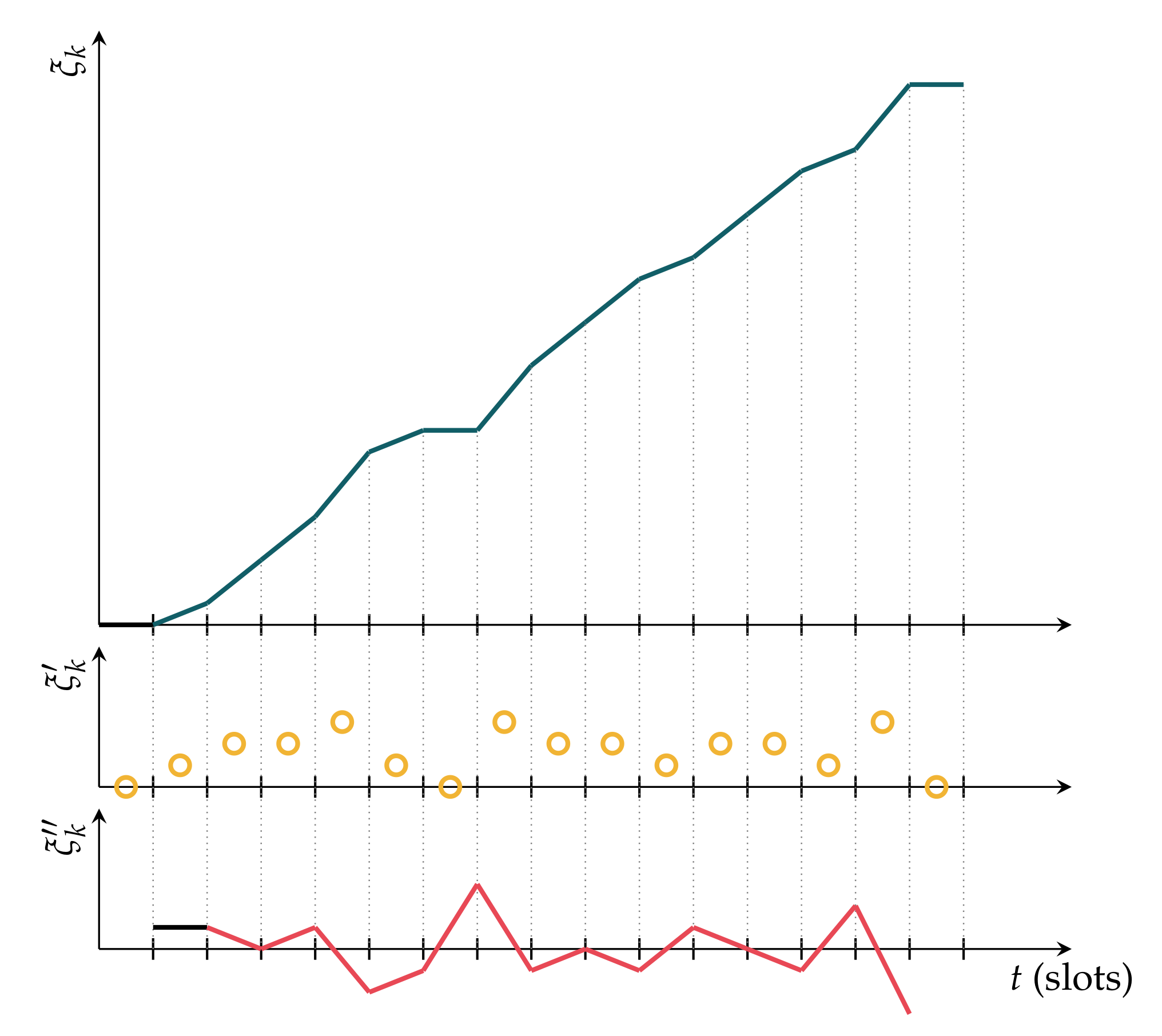
In order to illustrate the use of the proposed theoretical framework to evaluate the behavior of a routing protocol, Figure 1 shows a temporal sequence in an arbitrary node. In this figure, on the central axis we represent the packet sending events; on the upper axis we illustrate the evolution of the accumulated exposure. Finally, the axis at the bottom shows the pace of exposure accumulation. From a protocol point of view, the objective is twofold: first that the accumulated exposure of each node k, , is kept as low as possible; second, that the rhythm of exposure accumulation is compensated among all nodes within the network.
In order to consider the EMF exposure within a routing protocol, there are two key aspects to take into account: first, minimizing the total transmission power of a route, since it would reduce the overall EMF exposure within the whole scenario. On the other hand, by considering the exposure accumulation pace as a routing cost, the routing protocol is able to balance the traffic between various routes, avoiding exposure peaks over a particular area. The latter would be the consequence of keeping the same route, as it would be the case of traditional routing mechanisms. This exposure model allows considering dynamic route changes, by means of taking into account the temporal evolution of the exposure accumulation pace.
3.2. EMF-Aware Routing Algorithm
This section presents a routing algorithm that is used to better describe the behavior of the proposed routing protocol. We begin by posing an optimization problem, which considers both the instantaneous transmission power and the accumulated exposure. Afterwards, we propose an algorithm that can be used to solve the stated problem, exploiting graph theory and transformation techniques that we introduce for taking into account the two aforementioned parameters or routing metrics.
3.2.1. Network Model
The main distinctive characteristic of the proposed model is the need to consider both the instantaneous and accumulated transmitted power as routing metrics. The minimization of the transmission power would yield a reduction of the overall exposure within the whole scenario, but it would not avoid the appearance of exposure peaks, as well as great variability between different network areas. In order to avoid this, we need to also consider the accumulated transmitted power (or a function of it), as a proxy of the EMF exposure induced by each node. Hence, those nodes that have caused a higher exposure should be avoided in the future establishment of additional routes, thus leading to a fairer exposure distribution throughout the whole scenario. Note that the metrics used in this section are abstract, since the network model aims to integrate the two previously mentioned costs.
The network is modeled as a graph , where is the set of vertices and the set of the corresponding edges. We assume that two nodes are connected if the euclidean distance between them is shorter than the coverage area of the corresponding communication technology. Since the two routing metrics that we seek to optimize have different characteristics, they are attributed to either nodes or edges:
- Node accumulated exposure : this cost represents the accumulated exposure that has been induced by a node i up to a certain time. In this sense, it does not depend on the amount of traffic traversing a node at a particular time, since we are interested in just considering its transmission history. It is worth noting that the proposed routing framework would allow using different definitions of this cost, provided it remains independent of the traffic currently traversing the node. Since the EMF exposure grows with the transmission power, we will later consider to be proportional to the power transmitted by the node until a particular moment. Nevertheless, more accurate models could be used, for instance considering advanced antenna patterns, or user density around the node;
- Edge power exposure : this reflects the transmission power that the node requires to send a packet to the next hop through an edge e. It is therefore attributed to each of the edges. should be proportional to the traffic load over every link, since the more a node is traversed by traffic, the more packets it will need to forward. This way, we can define the cost of an edge e connecting two nodes as ; where is the required transmission power, and represents the traffic load in that edge.
Given the fact that our approach also assigns a cost to each node, we need to apply some network transformations before describing the algorithm, which will be used to establish the optimum routes. The reason for this is that most of the routing algorithms assume just edge costs, and so we introduce virtual edges to bear the cost . For our algorithm, each node i is split into two virtual vertices, which are then connected with an edge, having a cost : and , ingress and egress, respectively. The incoming edges at the original node n are now connected to , while the outgoing edges are now starting at .
As an illustrative example, Figure 2 shows the transformation applied to a simple graph of three nodes. Here, and are the traffic load and the required transmission power, between nodes i and j, respectively. On the other hand, models the overall exposure caused by node i up to a certain time. It can be easily inferred that the proposed transformation increases the complexity of the graph; if we start from an initial graph , we obtain a new one , where and .
3.2.2. An Optimization Problem to Minimize the EMF Exposure
Once we have presented the network model, we pose the optimization problem that needs to be solved, in order to establish those routes that would minimize the exposure. Since the overall cost (at least the one related to the transmission power) is proportional to the flow traversing an edge, we can state a problem similar to the Minimum Cost Flow Problem (MCF) one, whose main goal is to distribute the overall traffic throughout the graph, so that the global transportation cost is minimized. We represent values assigned to edges using the indexes of the nodes connected by the corresponding edge. This way, the edge connecting nodes i and j are represented by the pair . Then, for any edge in graph G, the problem can be expressed analytically as follows:
where and represent the cost per flow unit and the edge capacity, respectively; accounts for the traffic originated () or received () by each node; is the flow traversing every link of the graph. Constraint (6a) corresponds to the flow balance at every node (if equals 0, the node is neither a source or a sink), constraint (6b) ensures that the edge capacities are respected, and constraint (6c) ensures that the global flow balance is maintained.
3.2.3. The Algorithm That Addresses the Minimization Problem
There exist various algorithmic solutions for the minimum cost flow problem. Since we are more interested in the network model, rather than in the particular technique to solve it, we make use of a classical solution, namely the Cycle Canceling Algorithm (CCA). This algorithm exploits the optimality property, which establishes that a feasible solution is optimal if, and only if, the residual graph has no negative cycles [31]. The basic operation of the algorithm is described in Algorithm 1, where represents the residual capacity of the edge .
The aforementioned algorithm was originally introduced for networks having one single (source, destination) pair. In order to handle more realistic scenarios, where a number of nodes (gateways) might provide access to external networks, we propose adding two additional virtual nodes. A overall virtual source is connected to the actual traffic sources, while the real gateways are attached to a virtual destination that receives all the traffic. We fix the capacity of the links between the virtual and the real sources to one unit, ensuring that the sources are not generating more than one traffic flow. Besides, there is no upper limit for the amount of traffic on the link between gateways and the virtual destination. This way, although we could consider an arbitrary number of sources and gateways, the algorithm just needs to solve a problem with one single (source, destination) pair.
| Algorithm 1:Cycle Canceling Algorithm. |
| Require: |
| 1: Establish possible one flow |
| 2: while contains a negative cycle do |
| 3: Identify one negative cycle |
| 4: |
| 5: Increment flow units in the flow and update |
| 6: end while |
It is worth pointing out that, according to the graph transformation presented in Section 3.2.1, the cost of the virtual edges that are added (the ones connecting the ingress and the egress virtual nodes) should not be proportional to the flow, since these edges are meant to model the exposure accumulated at the current real node level, up to now. It follows that, we can define the cost as follows:
where is the transmission power, used by node i to reach node j, is a constant factor, represents the accumulated exposure of node i, and is the amount of flow traversing the link . In order to implement this, we heuristically modify the cost of the virtual links during the algorithm execution according to Equation (7), so that they are always constant. Although this could break the isotonicity of the corresponding graph, the obtained results empirically show that this approach was indeed valid.
3.3. EMF-Aware AODV Protocol
In this section we describe the basic principles of the proposed EMF-aware routing protocol, the so-called EA-AODV, which is theoretically grounded by the algorithm described in Section 3.2. Our implementation is based on the well known AODV protocol, whose operation has been modified to account for the new EMF related metrics. Hereinafter, we introduce the most significant protocol procedures, which are able to disseminate the evolution of the accumulated exposure, as well as the messages format. Other procedures that are not mentioned (i.e., neighbor discovery) are inherited from AODV. The reader may refer to the AODV specification in [7] for a detailed description.
Before describing the protocol in detail, we highlight some general considerations, with a clear impact on the protocol’s specification and implementation. We assume that nodes are able to dynamically adapt their transmission power, according to the link with their neighbors (next hop) and that the protocol is itself aware of such power, leveraging a cross-layer solution. An off-line training procedure was carried out in order to establish the power required to reach the next hop.
3.3.1. Signaling in EA-AODV
Regarding the signaling that the protocol uses, all messages carry the protocol version and message type fields. The former is included for future protocol modifications, and the latter allows distinguishing between the following messages:
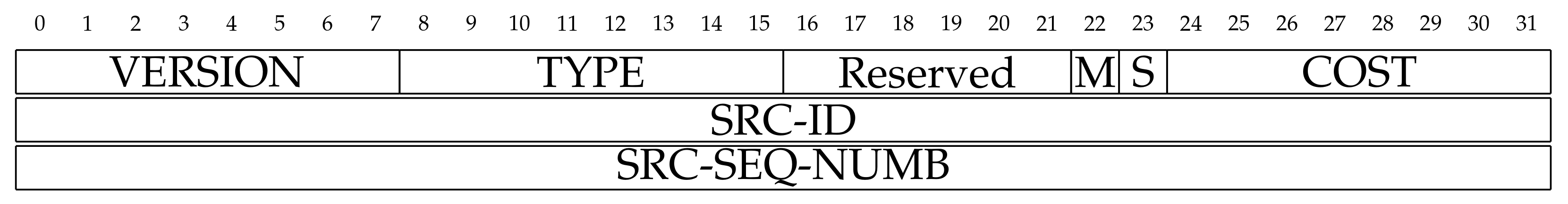
- HELLO: this message is periodically broadcasted with a twofold purpose. First, it allows neighbor discovery. Furthermore, we also use it to notify about a change in the node’s cost, due to an accumulated exposure modification. Figure 3 depicts the fields of this message. As can be seen, it includes two flags to indicate the role of the message: M determines whether the packet is used for neighbor discovery purposes (M = 0) or for notifying a change in the corresponding cost (M = 1). In the latter case, the S flag indicates the sign of such modification (0 or 1 for positive or negative change, respectively). Finally, the COST field carries the corresponding value;
- ROUTE_DISC: a broadcast message initiated by a source to find the route to a particular destination. Each node receiving this packet forwards it, until the packet reaches its destination. It carries the route accumulated costs, so as to populate it during the route discovery process. Each node increments the cost, proportionally to the transmission power that would have been required by the previous node to reach it. The fields of this type of message can be observed in Figure 4;
- DISC_ACK: this message follows a ROUTE_DISC, and it is sent by the destination as a unicast transmission towards the corresponding source. Its format corresponds to the one presented for the ROUTE_DISC message, the only difference being in the corresponding TYPE field. Since the nodes follow the same procedure as the one depicted for the management of the ROUTE_DISC message, the protocol is able to handle asymmetric links, in which the power required to send a packet depends on the particular direction. The fields of this type of message can be observed in Figure 4;
- REPORT: used to disseminate a cost change, either an increase or a decrease of the accumulated exposure. Although the accumulated exposure does not physically decrease, the protocol considers this option to include aging functions. For instance, if a node is not used for a while, the cost related to the accumulated exposure can be reduced to foster the use of such a node. It thus follows a HELLO with M = 1, and it is propagated to ensure that all affected nodes receive the information. Figure 5 illustrates the format of this message.
One of the main novel aspects of the proposed protocol is that it is able to dynamically manage the dynamic route costs, caused by the evolution of the accumulated exposure, as was previously done for the algorithmic analysis in Section 3.2. In what follows, we thoroughly depict how the actual calculation is carried out. First, the evolution of the cost with respect to the accumulated exposure does not follow any particular pattern, thus resulting in an asynchronous behavior. Furthermore, each node locally stores a routing table whose entries are identified by the destination/next-hop pair obtained during the route establishment procedure. Each route entry is linked to a timer that is re-started every time the entry is used. This way unused entries are removed, and the size of the table is kept small. We have extended the legacy AODV route table format, adding an additional field to represent the route state, which uses the following values:
- InUse: the route is being used to send locally generated data. This means that the node is the actual source of such an entry;
- Active: the route is being used to forward data. This is used when the node acts as a forwarding entity;
- Active_InUse: this state applies when the two previous conditions apply;
- Valid: the entry is not currently being used, but it has not yet expired.
3.3.2. Updating the Cost of a Node in EA-AODV
Figure 6 shows the message exchange that would be triggered upon a change of a node’s cost. We assume that there already existed a route from A to D, B and C being intermediate nodes. At a certain time, C needs to inform about a modification of the accumulated exposure, for instance upon crossing a predefined threshold. This would eventually impact the cost stored at the routing tables at the remaining nodes within the route. A being the source, it has an InUse route to D, while the state of the corresponding entry in both B and C is Active.
First, C sends a HELLO message with the flag M = 1, informing about a cost change. Upon receiving it, B and D check whether they have any route entry with an Active state using C as the next hop. In this particular example, D does not have any affected entry, and the message is thus silently discarded. On the other hand, when B receives the HELLO message, it confirms that it actually has an Active entry with C as the next hop. First, it updates the cost stored to reach D, increasing or decreasing (as represented by the ±symbol) it according to the S flag in the HELLO message. A cost decrease may be due to the adoption of aging functions, which would mitigate the effect of the cost associated to the accumulated exposure. Then, it builds a REPORT message: the field ROUTES_NUM carries the number of the routes that are affected by the received change, followed by the identifiers of all the corresponding destinations (i.e., ROUTE-DST-ID1). In this illustrative example, ROUTES_NUM equals 1, followed by the identifier of the corresponding destination, D. It is worth noting that a cost change in one node may impact several routes, so that it is necessary to notify affected nodes of each one.
Finally, when A receives the REPORT message, it parses the ROUTES_NUM field, checking whether it has any entry towards one of the identifiers that are included within it, having B as the next hop. In Figure 6, there is a match with an entry towards D, and its cost is therefore modified, according to the information carried in the REPORT message. In addition, A would also forward it, if the entry would be either Active or Active_InUse.
Another key issue is how the routing protocol calculates the value of the cost of a node () and notifies its change. This cost is computed as a function that depends on the number of transmitted packets until that moment, and the corresponding transmission power required to send each of them. As mentioned before, different functions could be assumed, depending on how the exposure is modeled (i.e., effect of antenna pattern). On the other hand, in order to avoid the flooding of the network due to cost change dissemination, cost change notifications are limited by means of thresholds and temporal windows.
4. Results
In this section we evaluate the proposed EMF-aware routing framework. First, we analyze the performance of the proposed routing algorithm, comparing it with legacy solutions. Then, the behavior of EA-AODV is studied by means of an extensive simulation campaign. To this end, the EA-AODV protocol has been implemented within the NS-3 framework, based on the existing AODV implementation.
4.1. Network Model Analysis
In this section we present the main results obtained from the evaluation of the algorithm that was presented in Section 3.2. We compare the proposed algorithm with a traditional one, based on the minimum cost, where costs are assigned to links according to the minimum transmission power required to reach the next node. Both algorithms are sequentially applied to the graph, in two different scenarios. This evaluation has been performed using the NS-3 framework, but without the actual implementation of EA-AODV. We start by generating the same traffic flows for each scenario and the algorithms are periodically executed, establishing the routes in all nodes. It is worth noting that the route definition in this case does not use protocol signaling, but it is set using the facilities provided by the simulation environment.
Before re-executing an algorithm, the information regarding the accumulated exposure is updated to appropriately capture the temporal evolution. We will study both the overall transmitted power, as well as how the exposure is accumulated. This way, the entire procedure will reflect the behavior of the protocol and reach the global optimum. This methodology allows the use of an ad-hoc implementation, which considers the temporal evolution due to different traffic flows, without using heavier tools, which would greatly impact the computation time.
We account for the accumulated exposure with the variable , which is used as a proxy of the physical exposure. To this end, the value of for a given node is defined as the power that such a node transmits within a given time interval. We assume that all flows are alike, so that if a node is part of a route (i.e., source, destination or relaying entity) the exposure induced by each node to its neighborhood grows linearly with the number of flows traversing it. Thus, the value of in each node increases by a constant value for every flow traversing the node.
The performance of the proposed algorithm is assessed by comparing it with that yielded by a minimum power algorithm, where the selected route is the one that requires less power to send a packet from the source to the destination. This minimum power algorithm is a shortest-path search, in which the cost of each edge represents the transmission power required to get to the next hop, without taking into account the overall flow traversing that particular edge. We will refer to these two approaches as EMFaware and MinPower, respectively.
This analysis aims to study how the proposed algorithm is able to yield a reduction of both the transmission power and the accumulated exposure.
We have studied scenarios with 50 nodes, having a wireless technology with a coverage range of 15 m, nodes being randomly deployed over a square area. Then we varied the density of nodes in the scenario by varying the side of the area, while keeping the coverage range of the nodes constant. The analyzed topologies are defined in Table 1. In all scenarios, four nodes are chosen as traffic sinks, a varying number of nodes play the role of traffic sources, and the rest are simple traffic forwarders. As can be seen, the scenarios differ in the number of traffic sources and density of nodes, while the overall number of nodes is kept at 50. The last row shows the Probability Density Function (PDF) of the number of gateways, or possible destinations, which can be reached in the corresponding scenarios.
In each topology we deploy four traffic sinks so as to maximize the covered area. The number of traffic sources, and thus the traffic flows, is varied, and routes are established without any preference that could favor any of them. From a network perspective, the destinations are considered as generic traffic gateways, which provide access to an external network. Note that this is reflected by the virtual destination, which was included in the network graph.
It is worth explaining how the accumulated exposure, , is measured. For each configuration (topology and number of sources) we run experiments of T time units, where . Then, we updated the accumulated exposure induced by each node according to the number of flows traversing it and recalculated the route. This way, if a node is selected in one route during the entire experiment, its accumulated exposure would reach a value of . On the other hand, the cost associated to the transmitted power is assumed to be proportional to the distance between the two nodes in the corresponding link. For each configuration we run 100 independent experiments of T time units to get statistically tight results.
We assign the cost values as follows: we increase from 0 to 15 the cost associated with the transmission power (the longer the distance, the higher power would be required to send packets over the link). Based on that particular range of values, we establish to be increased by 5 units for each flow forwarded by the node during a time slot. Besides, we do not give a higher priority to any of the two costs, i.e., accumulated exposure or instantaneous transmit power, with respect to one another. Although the costs selection is arbitrary, it will permit us to validate the performance of the EMFaware algorithm when compared to legacy ones, and to analyze its behavior.
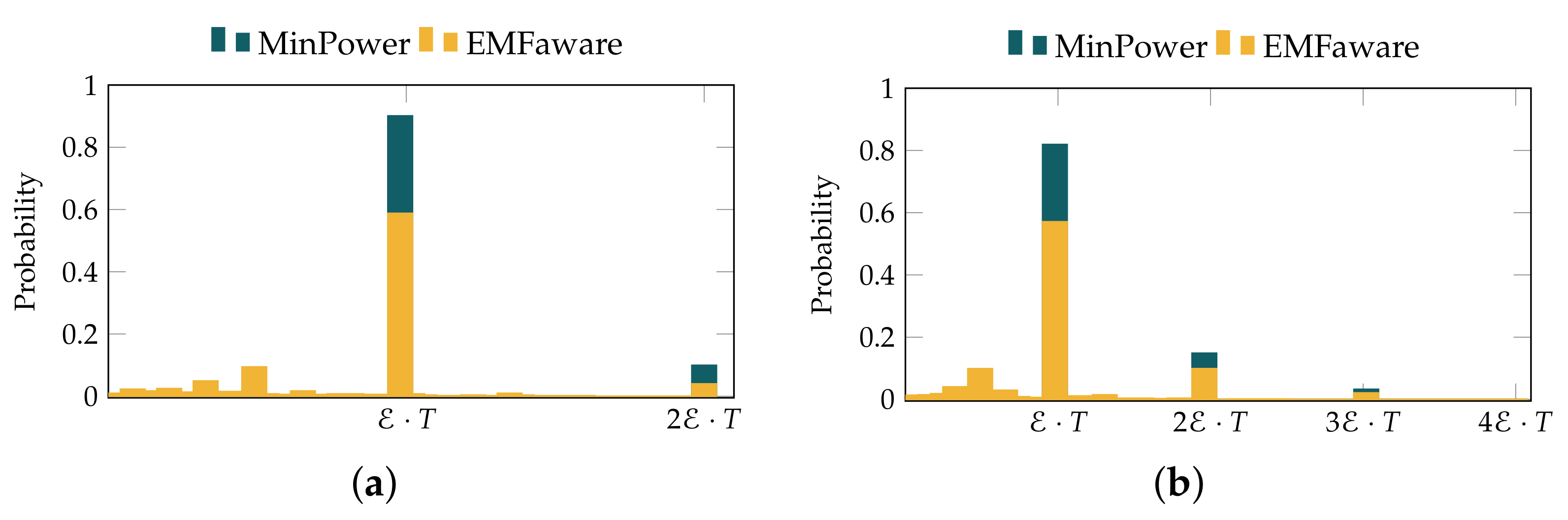
First, we studied the accumulated exposure at the different nodes during one experiment. Figure 7 shows the exposure PDF by considering all nodes for both algorithms and by using the topology, with both two and four sources. We can argue that the value corresponds to the exposure accumulated by a single node, if it had been active for one path during the whole experiment (duration T). Hence, a multiple of would reflect nodes that were active in more than one route. For instance, if the PDF at equals , that would imply that 10% of the nodes have been active in two routes during the whole experiment. This can be easily seen for the legacy shortest path (minimum power algorithm), which shows a discrete behavior. Indeed, the PDF is greater than 0 only in points multiple of , reflecting that the routes are kept static during the whole experiment, not changing due to the high accumulated exposure. On the other hand, the proposed EMFaware algorithm is able to balance the exposure. In particular, we can observe a relevant decrease on the PDF for , which is around and for the two and four sources scenarios, respectively. This reduction is reflected on the smaller bins, as can be seen for values within the interval , which were not observed for the legacy routing solution.
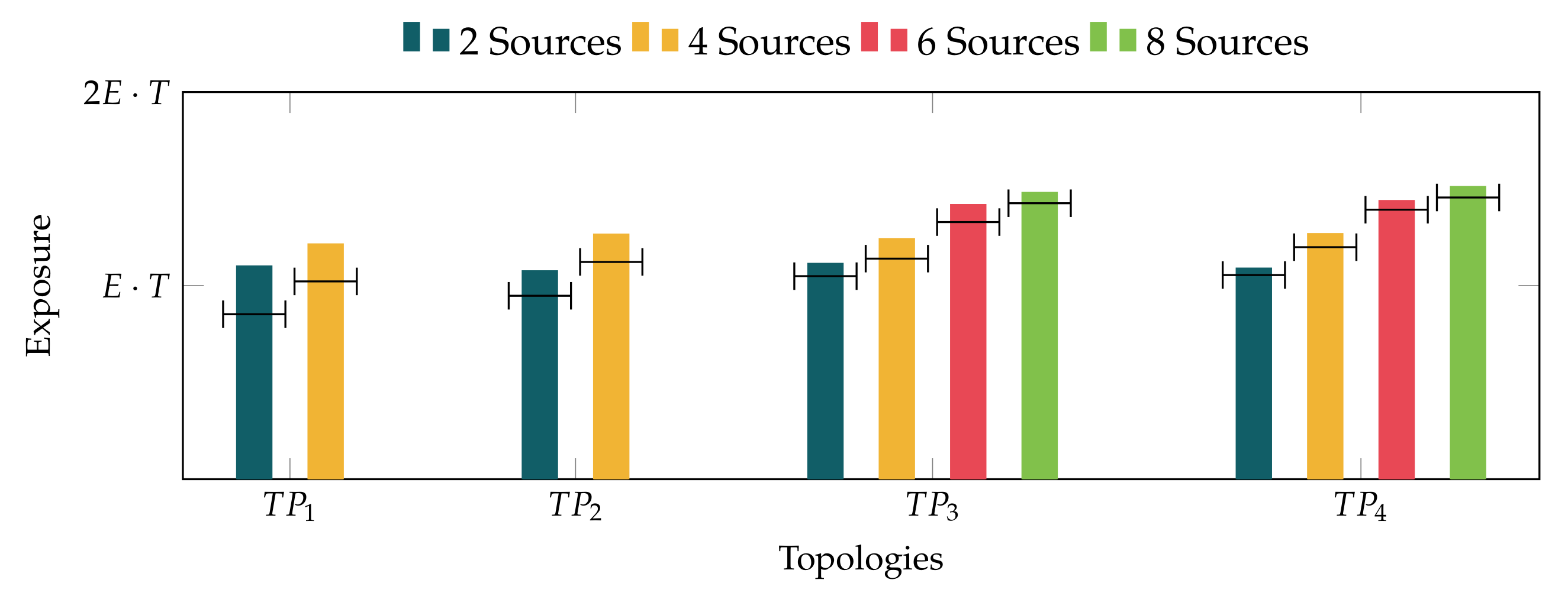
After validating that the EMFaware algorithm is actually able to modulate the accumulated exposure, the analysis is broadened to consider different topologies and traffic loads. In this context, Figure 8 shows the average value of the exposure, after 100 independent experiments, for different network deployments, considering various source nodes. The bars correspond to the values observed for the legacy shortest path minimum power solution, while the horizontal line represents the results brought by the proposed EMFaware solution. As can be seen, the degree of improvement for our novel algorithm reduces as long as we decrease the node density. The gain over topology is greater than the one observed for . The reason for this behavior is that lower dense topologies offer fewer routing alternatives, and so the proposed algorithm is not able to balance the accumulated exposure. Furthermore, the results also evince that there is not a clear impact of the number of traffic flows (simultaneous number of sources).
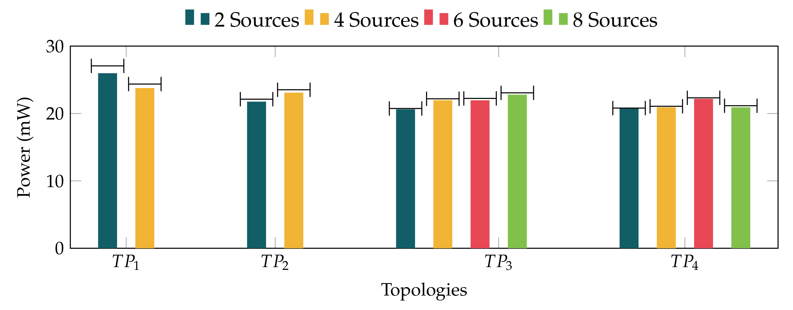
Taking into account that the exposure induced by the whole network should be directly related to the overall transmitted power, it is interesting to ascertain the performance of the proposed algorithm in terms of the overall transmitted power. This is important, especially since we are comparing it to a solution that seeks exactly the minimization of this parameter. Figure 9 shows the average value of the overall required transmission power. It is worth recalling that, in the case of the MinPower solution, the transmitted power does not change during the experiment, since the routes remain unchanged, while this might not be the case in the EMFaware algorithm. In this sense, when a change of route is enforced in the proposed solution, the required transmission power might be different. The results in Figure 9 evince that, although there is a slight penalization regarding the overall transmitted power, the increase is rather small, and it even becomes negligible for the scenarios with lower densities ( and ). For both solutions, we can clearly see that the smaller the density, the higher the required power, due to the longer distances that would be required in order to connect the source nodes to one of the available gateways.
4.2. Dynamic Traffic Flows
We now analyze the performance of the proposed solution in a more dynamic setup, where traffic sources are changed during the experiment. We carry out this analysis only over the scenario, using nine traffic destinations. The system configuration is similar to the one described in the previous section, except for the fact that traffic sources are changed every 25 time slots. This way, the accumulated exposure of a node, being part of one route during the whole experiment, would be no greater than .
Over this setup we study the relationship between and in two different ways. First, we vary the growing pace of , so that its relative importance compared to also varies. In addition, we apply an aging function to , so that the effect of the accumulated exposure vanishes when a node is not traversed by any traffic flow. Table 2 shows the configurations we used. is computed as described earlier (proportional to the distance), while the accumulated cost of a node is increased by , each time unit, for each flow traversing the node. For convenience, we use instead of . Then if a node is not used by any route, its accumulated exposure cost is reduced by units, each time slot. Altogether, in each slot t every node updates the accumulated exposure metric, , as shown in Equation (8).
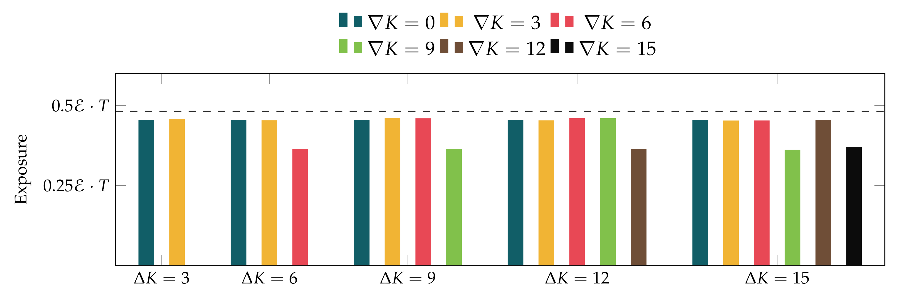
Figure 10 depicts the average value of the accumulated exposure obtained from 100 independent runs. It is represented using the generic quantity , to allow a fair comparison between the different configurations. In general we can see a negative impact of changing the traffic sources. In this sense, the exposure gain compared with the MinPower solution in Figure 10, when equals 0, is lower than the one observed in Figure 8. On the other hand, we can see that the use of aging functions has a positive effect. In short, when they are not used, nodes that were previously selected are unlikely to be part of a new route until other nodes reach similar accumulated exposure, which might lead to longer routes and therefore higher overall exposure. On the other hand, when we included the aging function, nodes might get re-selected sooner, lowering the overall system exposure. In addition, the results also evince that the aging function is only noticeable when is equal or greater that 6.
4.3. Protocol Evaluation
We now discuss the results that were obtained for the evaluation of the proposed EA-AODV protocol, described in Section 3.3. The protocol performance will be analyzed using different configurations, including the one that provides a power minimization behavior. Although legacy protocols that pursue minimizing transmitted power may have different signaling procedures, the obtained routes would be the same. In such a case, assuming that the user traffic is much higher than the signaling overhead, the results obtained with EA-AODV with minimum power configuration would be similar to the ones yielded by legacy solutions. On the other hand, we discard comparing EA-AODV with min-hop solutions (i.e., legacy AODV), since they do not seek minimizing the transmitted power, and the comparison would therefore be unfair.
We have carried out extensive simulations with the NS-3 [32] simulation framework, where the protocol has been implemented and integrated. We consider static scenarios comprising nodes equipped with 802.11 g wireless technology, with a maximum transmission power of 16 dBm.
The protocol itself does not strictly define the cost computation procedure, but it provides a framework to incorporate a dynamic cost adaptation scheme, including the mechanisms to appropriately propagate the corresponding changes. In particular, two different costs have been implemented within the protocol, based on the abstract ones that were previously used in Section 3.2. We have used the same naming as for the EMF-aware algorithm, and corresponds to the transmission power that is required to reach the next hop, while accounts for the accumulated exposure.
Differently to the algorithm evaluation, the costs in the protocol are calculated using actual power values. During the simulations, is established as the transmission power in mW, within the range , required to reach the next hop. On the other hand, is assessed every T seconds, by monitoring the total transmission power during the last slot. In order to be able to study the impact of assigning a different weight to either of the two costs, is scaled by a factor of . We will afterwards analyze how it impacts the protocol performance. The computed values are used during the route discovery procedure, where each node updates the corresponding cost values of the ROUTE_DISC message (see Section 3.3.1), locally computing and . Eventually, the source selects the route with minimum cost, and updates it according to the information provided during the cost update procedure, as was described Section 3.3.2.
As can be observed, the costs and in the protocol are particular definitions of the abstract ones that were used in Section 3.2. Furthermore, they both have a clear relationship with the theoretical framework presented in Section 3.1. Indeed, the exposure growing of each node (measured in mW), as well as the overall one (pertaining to the whole network), can be minimized by reducing the transmission power, i.e., with . On the other hand, (measured in mW/s), which modulates the pace at which the accumulated exposure varies, is considered by the latter cost component, . In particular, nodes that have transmitted more power during the last slot (higher mW/s), are penalized in the route decision process, and so the pace at which exposure accumulation varies is also taken into account by the proposed protocol.
We have first studied the protocol behavior over a simple network, in order to analyze the impact of the parameter. It is worth noting that the configuration with yields a minimum power solution.
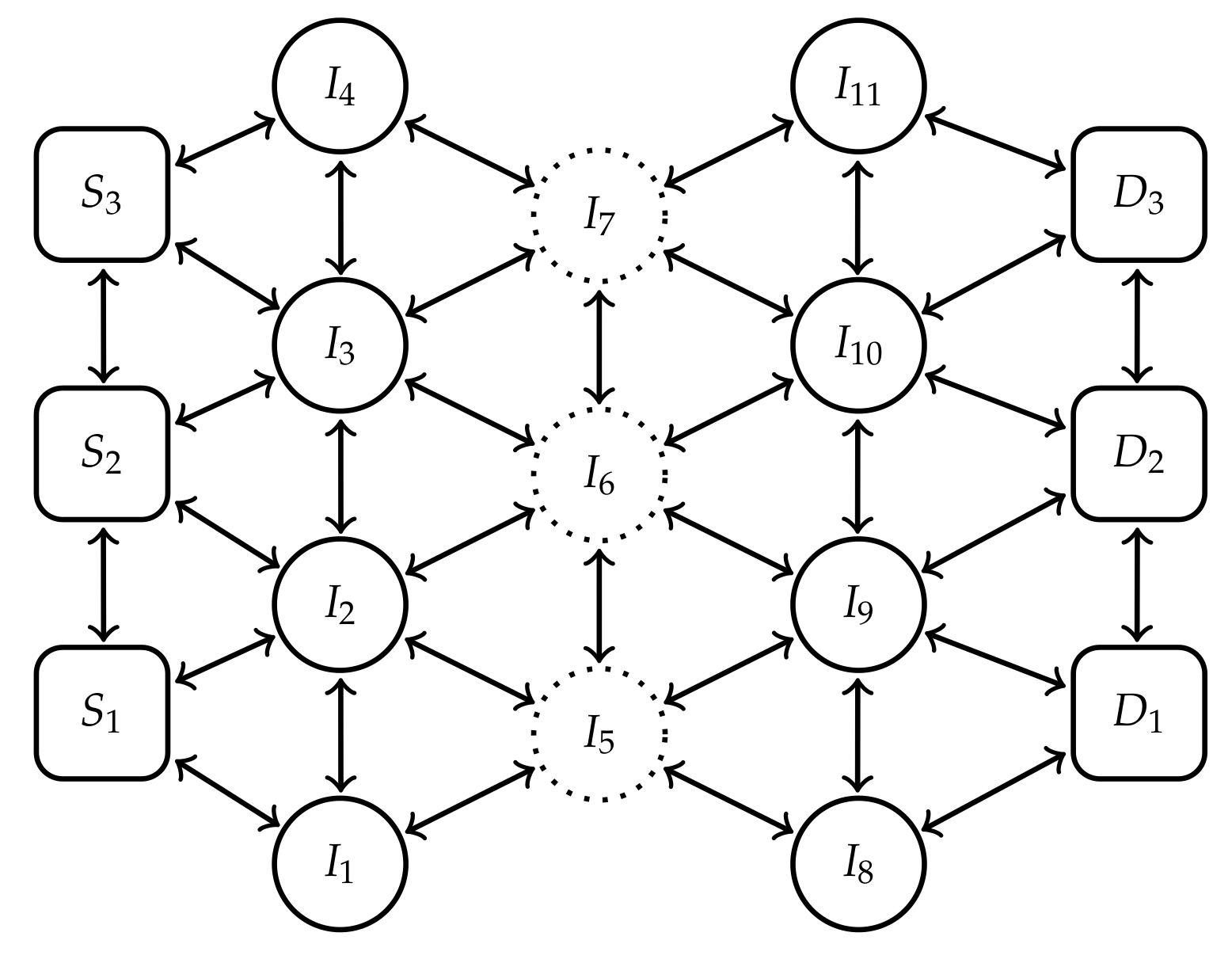
The corresponding network topology is shown in Figure 11, where three traffic sources send traffic to three potential gateways, with several available routing alternatives. A simulation of 120 s has been performed where each source sends one traffic flow, with a rate of 120 Kbps, to any gateway. In addition, we establish the time windows to assess the accumulated exposure to 5 s.
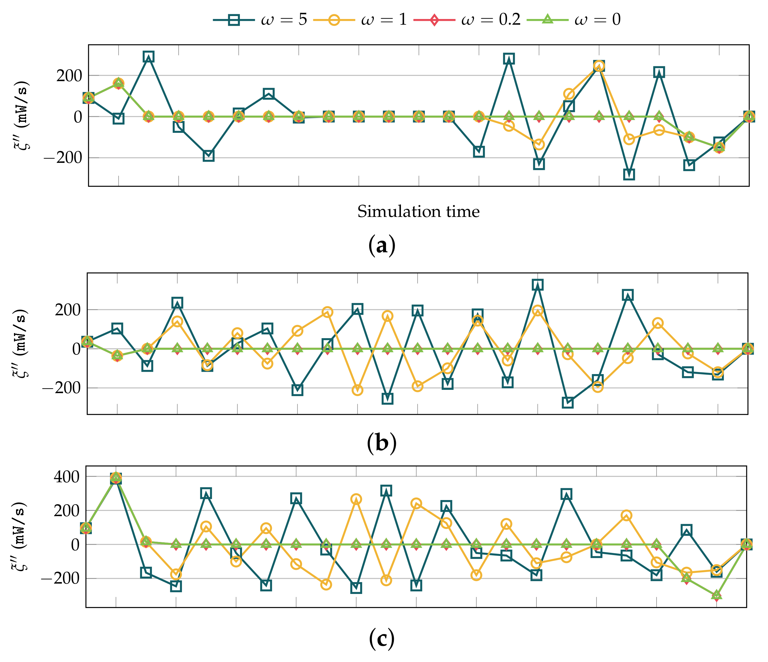
Figure 12 shows the rhythm at which the accumulated exposure grows for the three potential intermediate nodes (, , and ) over time, and for different values. The results show that for high values ( or ), the proposed protocol is actually able to modulate this corresponding rhythm, and so the parameter fluctuates during the simulation.
However, when the weight given to this cost decreases, the protocol favors the route with the lowest transmission power (minimum ), which is maintained throughout all the simulation, and so there is no change to the rhythm at which the accumulated exposure grows at the intermediate nodes.
Afterwards, we also evaluated the impact of the parameter over the accumulated transmitted power. Figure 13a shows its standard deviation for different values of . We can see a clear influence of the cost, resulting in a much more homogeneous exposure when the factor is higher. Besides, Figure 13b also illustrates the power that was transmitted by the entire network. In this setup we can also see a slight improvement for the highest value, which was not expected, since higher values usually lead to using routes that are not favoring the minimum power criterion. However, the traffic balancing between the various routes leveraged by this configuration causes fewer collision events and re-transmissions.
After assessing the correct behavior of the routing protocol, we have analyzed its performance over more complex scenarios, considering random topologies. We assume a square scenario of m2, where four arbitrary sources send traffic to any of the four gateways, which are deployed to maximize their coverage. We increase the number of intermediate nodes, and therefore the network density, from 50 to 200, and we modify the value of . We run 100 independent simulations for each value, and for the two different network densities (50 and 200 intermediate nodes). As was done with the algorithm evaluation previously discussed, we discard those network deployments where there is no route from each source to one of the available gateways. We also use the same traffic characteristics and window time (T) as in the previous analysis.
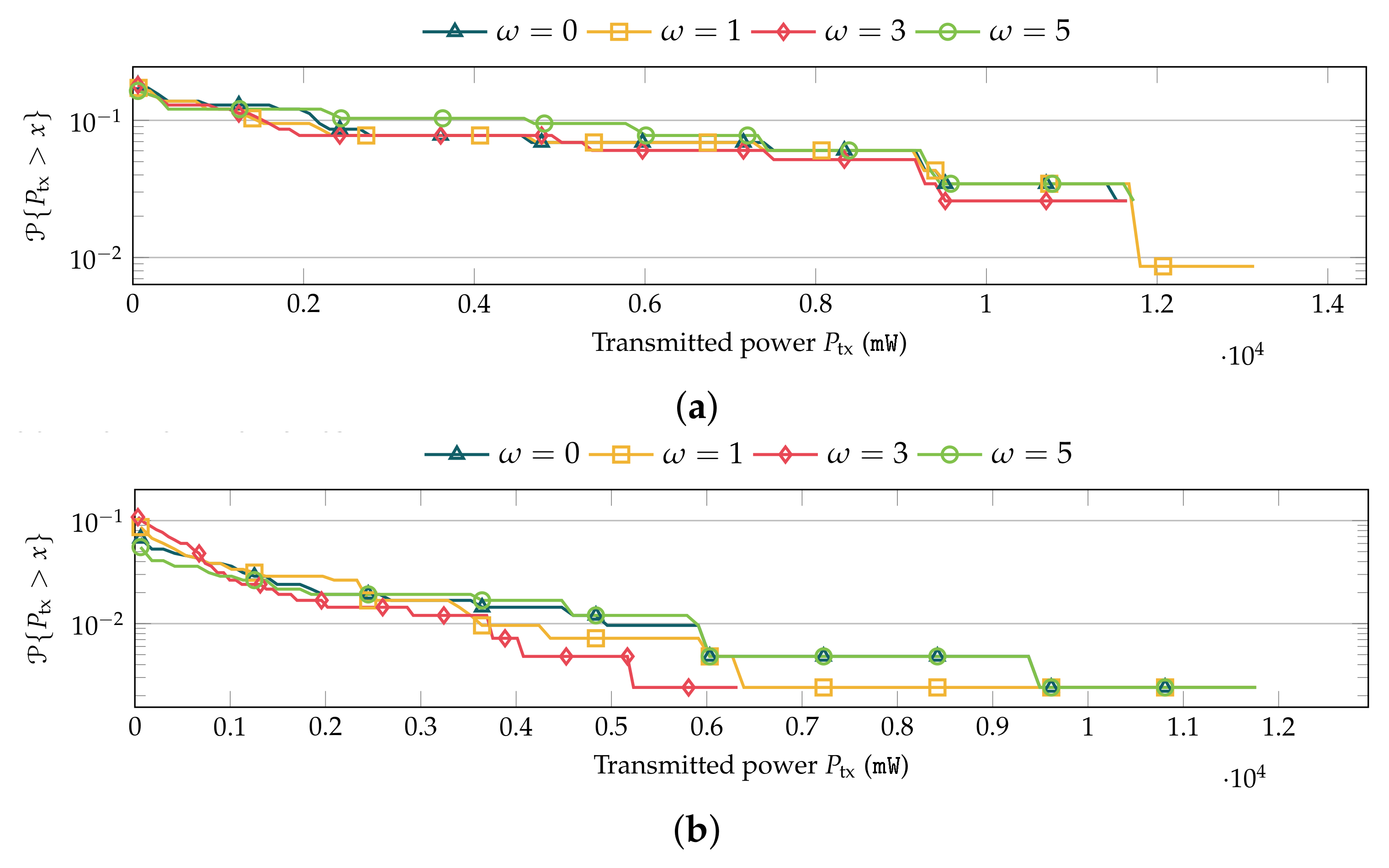
First, Figure 14 shows the Complementary Cumulative Distribution Function (CCDFs) of the power transmitted by each node during the whole experiment. As can be observed, there is a slight improvement when moderate weight ( and ) is given to the metric that considers the accumulated exposure, , while such an improvement is no longer evinced as we increase the weight (). This enhancement is slightly higher for more dense networks, as can be seen in Figure 14b for 200 intermediate nodes. In any case, the difference with the configuration in which the protocol just seeks the minimization of the transmitted power () is not very relevant.
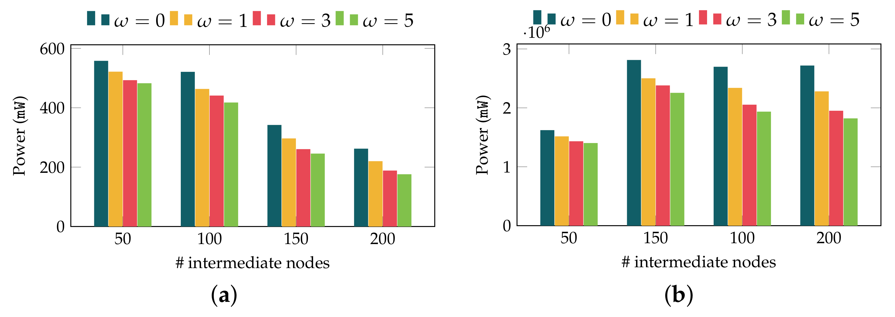
Afterwards, in Figure 15 we assessed the influence of the metric over the average and overall transmission power. Figure 15a shows the average transmitted power per node. We can observe a monotonic decrease of the average transmission power due to the fact that the denser the network, the more routing alternatives become available. This, in turn, implies that it is more likely to find routes requiring less power. The results show that the use of higher values leads to a clear benefit in terms of the transmitted power. Furthermore, the same effect can be observed for the overall transmitted power. Then, Figure 15b exhibits a behavior similar to the one seen for the standard deviation of the transmit power.
We can finally conclude that, for the considered network topologies, the use of the dynamic metric that accounts for the accumulated exposure yields a reduction of the total power transmitted by the complete network. This reduction is achieved by means of a fairer distribution of the exposure induced by the different nodes. This exposure distribution avoids concentrating traffic in some particular nodes or geographical areas, so leading to a certain traffic load balancing between the available paths. In turn, this reduces the number of wireless collisions and traffic retransmissions, causing the power savings that are evinced in the analyzed scenarios. On the other hand, we believe that this effect may not appear in other scenarios with lower density, and that it may have some impact in other QoS parameters, such as delay. A further analysis of this effect will be tackled in our future work.
In addition, we have also observed that the the proposed solution yields a certain traffic balance between the available paths. We have also validated the correct operation of the EA-AODV protocol, which provides an open implementation to include the EMF exposure in the routing procedure, where costs can be customized for both the accumulated exposure and instantaneous transmission power.
5. Conclusions
In this paper we have proposed a novel routing framework for wireless multi-hop networks, which considers minimizing the exposure to Electromagnetic Fields, leveraging an original and novel approach for these scenarios. In the last years we have observed a growing concern regarding the effects that EMF induced by wireless communications may have over people. Indeed, this concern has increased with the appearance of novel wireless technologies for 5G systems, such as mmWave. In order to address this, we have proposed an EMF-aware solution that can be used in multi-hop wireless networks, such as the ones used for D2D or WSN for Internet of Things (IoT).
We have carried out a holistic approach, combining both theoretical and simulation-based analysis. First, we studied the optimum performance by means of a novel algorithm based on graph theory. Afterwards, taking into account that the exposure cannot be directly embedded within a routing protocol, we have presented an analytical model of the exposure, where we identified a sensible metric that could be used in order to effectively reduce the exposure. Afterwards, we have presented the design and specification of a routing protocol that tackles the exposure reduction, and we assessed its performance by means of an extensive simulation campaign.
The results offer the evidence that the proposed solutions (both the algorithm and the protocol) are able to fairly balance the EMF exposure within the network, also yielding a decrease on the average exposure. We have also seen that the observed gain is more relevant for higher node densities, since the proposed approach benefits from a larger number of alternative paths. In addition, the analysis evinces that there is not a relevant trade-off in terms of the consumed power, and our solution roughly keeps the overall transmit power as the one that minimizes this particular metric. Moreover, the evaluation results show that the use of the dynamic cost that accounts for the accumulated exposure brings remarkable benefits, by reducing the average emitted power. On top of it, the same benefits can be observed in the overall transmitted power by the network. This reduction is obtained thanks to the fair distribution of the exposure induced by different nodes and so a better traffic balance among alternative paths.
In our future work, we will study the proposed scheme over more dynamic (adding mobility) and complex (with higher densities) scenarios. We will also look at the weights given to the two parameters, and their impact over the algorithm/protocol performance, assessing whether there is any optimum configuration that might yield better performances.
Author Contributions
Conceptualization, V.I., L.D., E.S. and R.A.; methodology, V.I. and L.D.; software, L.D.; formal analysis, V.I.; writing—original draft preparation, V.I. and L.D.; writing—review and editing, V.I., L.D., E.S. and R.A.; funding acquisition, E.S., R.A. All authors have read and agreed to the published version of the manuscript.
Funding
This work has received funding from the Spanish Government (Ministerio de Economía y Competitividad, Fondo Europeo de Desarrollo Regional, MINECO-FEDER) by means of the project FIERCE: Future Internet Enabled Resilient smart CitiEs (RTI2018-093475-AI00).
Data Availability Statement
Not applicable.
Conflicts of Interest
The authors declare no conflict of interest.
Abbreviations
The following abbreviations are used in this manuscript:
| NS-3 | Network Simulator 3 |
| D2D | device-to-device |
| QoS | Quality of Service |
| AODV | Ad hoc On-Demand Distance Vector Routing |
| EA-AODV | EMF Aware AODV |
| CCA | Cycle Canceling Algorithm |
| CCDF | Complementary Cumulative Distribution Function |
| ICNIRP | International Commission on Non-ionizing Radiation Protection |
| mmWave | Millimeter Waves |
| NRR | Nearest Neighbor Routing |
| MANET | Mobile Ad-hoc Networks |
| VANET | Vehicular Ad-hoc Network |
| MCF | Minimum Cost Flow Problem |
| EMF | Electromagnetic Fields |
| LEXNET | Low EMF Exposure Networks |
| EI | Exposure Index |
| WMN | Wireless Mesh Networks |
| WSN | Wireless Sensor Networks |
| Probability Density Function | |
| ETX | Expected Transmission Count |
| ETT | Expected Transmission Time |
| WCETT | Weighted Commutative Expected Transmission Time |
| MIC | Metric for Interference and Channel Switching |
| iAWARE | Interference Aware |
| EETT | Exclusive Expected Transmission Time |
| SAR | Specific Absorption Rate |
| IoT | Internet of Things |
Appendix A. Proof of the Continuous Individual Exposure
It is well-known that the area between 2 points, a and x, below the curve of any one variable function h that is derivable, can be formally expressed by means of the Riemann integral: . If we consider a to be a fixed initial real value and x to be variable, we get:
Now, if the function h is two times derivable, considering that we know the expression or shape of the function , we could similarly express as:
If we integrate this once again, between a and b, we get:
Appendix B. Proof of the Discrete Individual Exposure
Let h be a staircase function, the value of h in a point n, , can be expressed as the double summation of its second derivative as follows:
which, in turn, can be expressed as
Since it follows from Theorem 1 that the value of could only change in points , we have a stairlike function whose value is constant on each interval , where .
Thus, we can write the innermost integral of the double integral from Theorem 1 as a sum of integrals on each unit length interval, , where . Then, we can apply the mean value theorem for integrals for each integral from S to , and consequently follow the same two steps for the outermost integral. If we do the corresponding maths, we get to:
References
- Cisco and/or Its Affiliated. Cisco Annual Internet Report (2018–2023). 2018. Available online: https://www.cisco.com/c/en/us/solutions/collateral/executive-perspectives/annual-internet-report/white-paper-c11-741490.html (accessed on 13 January 2022).
- Internation Commission on Non-Ionizing Radiation Protection (ICNIRP). ICNIRP Guidelines For Limiting Exposure To Electromagnetic Fields (100 kHz to 300 GHz). 2020. Available online: https://www.icnirp.org/cms/upload/publications/ICNIRPrfgdl2020.pdf (accessed on 13 January 2022).
- Low Electromagnetic Field Exposure Networks. 2012. Available online: https://cordis.europa.eu/project/id/318273 (accessed on 13 January 2022).
- Wu, T.; Rappaport, T.S.; Collins, C.M. The human body and millimeter-wave wireless communication systems: Interactions and implications. In Proceedings of the 2015 IEEE International Conference on Communications (ICC), London, UK, 8–12 June 2015; pp. 2423–2429. [Google Scholar] [CrossRef] [Green Version]
- Nadeem, L.; Azam, M.A.; Amin, Y.; Al-Ghamdi, M.A.; Chai, K.K.; Khan, M.F.N.; Khan, M.A. Integration of D2D, Network Slicing, and MEC in 5G Cellular Networks: Survey and Challenges. IEEE Access 2021, 9, 37590–37612. [Google Scholar] [CrossRef]
- Tesanovic, M.; Conil, E.; De Domenico, A.; Aguero, R.; Freudenstein, F.; Correia, L.; Bories, S.; Martens, L.; Wiedemann, P.; Wiart, J. The LEXNET Project: Wireless Networks and EMF: Paving the Way for Low-EMF Networks of the Future. Veh. Technol. Mag. IEEE 2014, 9, 20–28. [Google Scholar] [CrossRef] [Green Version]
- Perkins, C.; Belding-Royer, E.; Das, S. Ad Hoc On-Demand Distance Vector (AODV) Routing. 2003. Available online: https://www.rfc-editor.org/info/rfc3561 (accessed on 13 January 2022).
- Abolhasan, M.; Abdollahi, M.; Ni, W.; Jamalipour, A.; Shariati, N.; Lipman, J. A Routing Framework for Offloading Traffic From Cellular Networks to SDN-Based Multi-Hop Device-to-Device Networks. IEEE Trans. Netw. Serv. Manag. 2018, 15, 1516–1531. [Google Scholar] [CrossRef]
- Pattnaik, P.K.; Panda, B.K.; Sain, M. Design of Novel Mobility and Obstacle-Aware Algorithm for Optimal MANET Routing. IEEE Access 2021, 9, 110648–110657. [Google Scholar] [CrossRef]
- Kacem, I.; Sait, B.; Mekhilef, S.; Sabeur, N. A New Routing Approach for Mobile Ad Hoc Systems Based on Fuzzy Petri Nets and Ant System. IEEE Access 2018, 6, 65705–65720. [Google Scholar] [CrossRef]
- Mohamed, E.M.; Elhalawany, B.M.; Khallaf, H.S.; Zareei, M.; Zeb, A.; Abdelghany, M.A. Relay Probing for Millimeter Wave Multi-Hop D2D Networks. IEEE Access 2020, 8, 30560–30574. [Google Scholar] [CrossRef]
- Feng, G.; Li, X.; Gao, Z.; Wang, C.; Lv, H.; Zhao, Q. Multi-Path and Multi-Hop Task Offloading in Mobile Ad Hoc Networks. IEEE Trans. Veh. Technol. 2021, 70, 5347–5361. [Google Scholar] [CrossRef]
- Wang, X.; Weng, Y.; Gao, H. A Low-Latency and Energy-Efficient Multimetric Routing Protocol Based on Network Connectivity in VANET Communication. IEEE Trans. Green Commun. Netw. 2021, 5, 1761–1776. [Google Scholar] [CrossRef]
- Youssef, M.; Ibrahim, M.; Abdelatif, M.; Chen, L.; Vasilakos, A. Routing Metrics of Cognitive Radio Networks: A Survey. Commun. Surv. Tutor. IEEE 2014, 16, 92–109. [Google Scholar] [CrossRef]
- Guerin, J.; Portmann, M.; Pirzada, A. Routing metrics for multi-radio wireless mesh networks. In Proceedings of the Telecommunication Networks and Applications Conference, ATNAC, Christchurch, New Zealand, 2–5 December 2007; pp. 343–348. [Google Scholar] [CrossRef] [Green Version]
- Iqbal, F.; Javed, M.; Iqbal, M. Diversity based review of Multipath Routing Metrics of Wireless Mesh Networks. In Proceedings of the Multi-Topic Conference (INMIC), 2014 IEEE 17th International, Karachi, Pakistan, 8–10 December 2014; pp. 320–325. [Google Scholar] [CrossRef]
- De Couto, D.S.J.; Aguayo, D.; Bicket, J.; Morris, R. A High-throughput Path Metric for Multi-hop Wireless Routing. Wirel. Netw. 2005, 11, 419–434. [Google Scholar] [CrossRef]
- Draves, R.; Padhye, J.; Zill, B. Routing in Multi-radio, Multi-hop Wireless Mesh Networks. In Proceedings of the 10th Annual International Conference on Mobile Computing and Networking, Philadelphia, PA, USA, 26 September–1 October 2004; ACM: New York, NY, USA, 2004; pp. 114–128. [Google Scholar] [CrossRef]
- Jiang, W.; Liu, S.; Zhu, Y.; Zhang, Z. Optimizing Routing Metrics for Large-Scale Multi-Radio Mesh Networks. In Proceedings of the Wireless Communications, Networking and Mobile Computing, WiCom, Shanghai, China, 21–25 September 2007; pp. 1550–1553. [Google Scholar] [CrossRef]
- Yang, Y.; Wang, J.; Kravets, R. Interference-Aware Load Balancing for Multihop Wireless Networks; Tech. Rep. UIUCDCS-R-2005-2526; Department of Computer Science, University of Illinois at Urbana-Champaign: Urbana, IL, USA, 2005. [Google Scholar]
- Subramanian, A.; Buddhikot, M.; Miller, S. Interference aware routing in multi-radio wireless mesh networks. In Proceedings of the Wireless Mesh Networks, Reston, VA, USA, 25–28 September 2006; pp. 55–63. [Google Scholar] [CrossRef]
- Auer, G.; Giannini, V.; Desset, C.; Godor, I.; Skillermark, P.; Olsson, M.; Imran, M.; Sabella, D.; Gonzalez, M.; Blume, O.; et al. How much energy is needed to run a wireless network? Wirel. Commun. IEEE 2011, 18, 40–49. [Google Scholar] [CrossRef]
- Correia, L.; Zeller, D.; Blume, O.; Ferling, D.; Jading, Y.; Godor, I.; Auer, G.; Van der Perre, L. Challenges and enabling technologies for energy aware mobile radio networks. Commun. Mag. IEEE 2010, 48, 66–72. [Google Scholar] [CrossRef]
- Veeraiah, N.; Ibrahim Khalaf, O.; Prasad, C.V.P.R.; Alotaibi, Y.; Alsufyani, A.; Alghamdi, S.A.; Alsufyani, N. Trust Aware Secure Energy Efficient Hybrid Protocol for MANET. IEEE Access 2021, 9, 120996–121005. [Google Scholar] [CrossRef]
- Ibrahim, A.; Ngatched, T.M.N.; Dobre, O.A. Using Bender’s Decomposition for Optimal Power Control and Routing in Multihop D2D Cellular Systems. IEEE Trans. Wirel. Commun. 2019, 18, 5050–5064. [Google Scholar] [CrossRef]
- Lee, S.W.; Ali, S.; Yousefpoor, M.S.; Yousefpoor, E.; Lalbakhsh, P.; Javaheri, D.; Rahmani, A.M.; Hosseinzadeh, M. An Energy-Aware and Predictive Fuzzy Logic-Based Routing Scheme in Flying Ad Hoc Networks (FANETs). IEEE Access 2021, 9, 129977–130005. [Google Scholar] [CrossRef]
- Das, A.; Das, N. Multihop D2D Communication to Minimize and Balance SAR in 5G. In Proceedings of the 2020 International Conference on COMmunication Systems NETworkS (COMSNETS), Bengaluru, India, 7–11 January 2020; pp. 590–593. [Google Scholar] [CrossRef]
- Iancu, V.; Diez, L.; Rodriguez de Lope, L.; Slusanschi, E.; Aguero, R. A reward-based routing protocol to reduce the EMF exposure over wireless mesh networks. In Proceedings of the Wireless Days (WD), 2014 IFIP, Rio de Janeiro, Brazil, 12–14 November 2014; pp. 1–4. [Google Scholar] [CrossRef]
- Diez, L.; Igareda, J.; Iancu, V.; Slusanschi, E.; Aguero, R. Routing algorithm to fairly distribute the exposure to electromagnetic fields over wireless mesh networks. In Proceedings of the 2015 IEEE 11th International Conference on Wireless and Mobile Computing, Networking and Communications (WiMob), Abu Dhabi, United Arab Emirates, 19–21 October 2015; pp. 468–473. [Google Scholar] [CrossRef]
- Rathan, K.; Roslin, S.E. A survey on routing protocols and load balancing techniques in Wireless Mesh Networks. In Proceedings of the 2017 International Conference on Intelligent Computing and Control (I2C2), Coimbatore, India, 23–24 June 2017; pp. 1–5. [Google Scholar] [CrossRef]
- Ahuja, R.K.; Magnanti, T.L.; Orlin, J.B. Network Flows: Theory, Algorithms, and Applications; Prentice-Hall, Inc.: Upper Saddle River, NJ, USA, 1993. [Google Scholar]
- Riley, G.F.; Henderson, T.R. The ns-3 Network Simulator. In Modeling and Tools for Network Simulation; Springer: Berlin/Heidelberg, Germany, 2010; pp. 15–34. [Google Scholar] [CrossRef]
Figure 1.
Evolution of the exposure and its second derivative upon transmission events.

Figure 2.
Example of transformation of a graph embracing 3 nodes. Original and transformed graph are shown in (a,b), respectively.
Figure 2.
Example of transformation of a graph embracing 3 nodes. Original and transformed graph are shown in (a,b), respectively.

Figure 3.
Structure of the HELLO message.

Figure 4.
Message structure of ROUTE_DISC and DISC_ACK.

Figure 5.
Structure of the REPORT message.

Figure 6.
Sequence diagram of cost change. Dashed lines are used to show lifetimes of the involved nodes, rectangles depict operations performed by the node, and arrows represent messages sending.
Figure 6.
Sequence diagram of cost change. Dashed lines are used to show lifetimes of the involved nodes, rectangles depict operations performed by the node, and arrows represent messages sending.

Figure 7.
Joint probability distribution of accumulated exposure for topology , accounting for the values obtained in every node. (a) Two sources. (b) Four sources.
Figure 7.
Joint probability distribution of accumulated exposure for topology , accounting for the values obtained in every node. (a) Two sources. (b) Four sources.

Figure 8.
Mean value of the reached exposure per experiment. We represent the values yielded by the EMFaware and MinPower algorithms with markers and bars, respectively.
Figure 8.
Mean value of the reached exposure per experiment. We represent the values yielded by the EMFaware and MinPower algorithms with markers and bars, respectively.

Figure 9.
Mean power obtained per generated route. We represent the values yielded by the EMFaware and MinPower algorithms with markers and bars, respectively.
Figure 9.
Mean power obtained per generated route. We represent the values yielded by the EMFaware and MinPower algorithms with markers and bars, respectively.

Figure 10.
Average exposure reached at the end of a experiment. We represent the values yielded by the EMFaware and MinPower algorithms with bars and dotted line, respectively.
Figure 10.
Average exposure reached at the end of a experiment. We represent the values yielded by the EMFaware and MinPower algorithms with bars and dotted line, respectively.

Figure 11.
Network topology with three sources and three destinations.

Figure 12.
Evolution of the second derivative metric. (a) Node . (b) Node . (c) Node .

Figure 13.
Power transmission statistics upon variation of . (a) Standard deviation. (b) Total power transmitted.
Figure 13.
Power transmission statistics upon variation of . (a) Standard deviation. (b) Total power transmitted.

Figure 14.
CCDF of the power transmitted by each node. (a) 50 intermediate nodes. (b) 200 intermediate nodes.
Figure 14.
CCDF of the power transmitted by each node. (a) 50 intermediate nodes. (b) 200 intermediate nodes.

Figure 15.
Random topology: power transmission statistics. (a) Average transmitted power. (b) Total transmitted power.
Figure 15.
Random topology: power transmission statistics. (a) Average transmitted power. (b) Total transmitted power.


Table 1.
Configuration of the static topology.
| Topology | ||||
|---|---|---|---|---|
| TP1 | TP2 | TP3 | TP4 | |
| Sources | ||||
| Area m2 | ||||
| PDF of reachable gateways |  | |||
Table 2.
Costs configuration.
| Cost Parameter | Value |
|---|---|
| P | distance (m) |
Publisher’s Note: MDPI stays neutral with regard to jurisdictional claims in published maps and institutional affiliations. |
© 2022 by the authors. Licensee MDPI, Basel, Switzerland. This article is an open access article distributed under the terms and conditions of the Creative Commons Attribution (CC BY) license (https://creativecommons.org/licenses/by/4.0/).
Share and Cite
MDPI and ACS Style
Iancu, V.; Diez, L.; Sluşanschi, E.; Agüero, R. Balancing the Electromagnetic Field Exposure in Wireless Multi-Hop Networks: An EMF-Aware Routing Scheme. Mathematics 2022, 10, 668. https://0-doi-org.brum.beds.ac.uk/10.3390/math10040668
AMA Style
Iancu V, Diez L, Sluşanschi E, Agüero R. Balancing the Electromagnetic Field Exposure in Wireless Multi-Hop Networks: An EMF-Aware Routing Scheme. Mathematics. 2022; 10(4):668. https://0-doi-org.brum.beds.ac.uk/10.3390/math10040668
Chicago/Turabian StyleIancu, Voichiţa, Luis Diez, Emil Sluşanschi, and Ramón Agüero. 2022. "Balancing the Electromagnetic Field Exposure in Wireless Multi-Hop Networks: An EMF-Aware Routing Scheme" Mathematics 10, no. 4: 668. https://0-doi-org.brum.beds.ac.uk/10.3390/math10040668
Note that from the first issue of 2016, this journal uses article numbers instead of page numbers. See further details here.