
A Discrete Dynamics Approach to a Tumor System
by
 , , ,
, , ,
Tareq Saeed
1 ,
,
Kamel Djeddi
2,
Juan L. G. Guirao
1,3,* ,
,
Hamed H. Alsulami
1 and
Mohammed Sh. Alhodaly
1 1
Nonlinear Analysis and Applied Mathematics (NAAM)—Research Group, Department of Mathematics, Faculty of Science, King Abdulaziz University, P.O. Box 80203, Jeddah 21589, Saudi Arabia
2
Laboratory of Dynamical Systems and Control, Department of Mathematics and Computer Science, Larbi Ben MHidi University, Oum El Bouaghi 4000, Algeria
3
Departamento de Matemáca Aplicada y Estadística, Universidad Politécnica de Cartagena, 30202 Cartagena, Spain
*
Author to whom correspondence should be addressed.
Mathematics 2022, 10(10), 1774; https://0-doi-org.brum.beds.ac.uk/10.3390/math10101774
Submission received: 28 February 2022
/
Revised: 9 May 2022
/
Accepted: 19 May 2022
/
Published: 23 May 2022
(This article belongs to the Special Issue Mathematical Models and Applications in Cancer)
Abstract
:In this paper, we present a cancer system in a continuous state as well as some numerical results. We present discretization methods, e.g., the Euler method, the Taylor series expansion method, and the Runge–Kutta method, and apply them to the cancer system. We studied the stability of the fixed points in the discrete cancer system using the new version of Marotto’s theorem at a fixed point; we prove that the discrete cancer system is chaotic. Finally, we present numerical simulations, e.g., Lyapunov exponents and bifurcations diagrams.
MSC:
37C80; 37G15; 37C301. Introduction
Cancer is a group of diseases involving abnormal cell growth. These cells could form a mass known as a tumor. A malignant tumor means it could invade or spread into nearby tissues. Therefore, cancer cells (linked with tumor growth) could reach distant parts of the body and form a new tumor (far from the original one). A benign tumor means the tumor can grow but not spread.
Many authors have used mathematical models. The main components of these models involve interactions among three types of cells, cancer cells with healthy host cells, and cells of the immune system. These interactions may lead to different outcomes. In the literature, there are several reviews on mathematical systems applied to tumor dynamics, e.g., [1,2,3,4].
An approach using a discrete-time system is better to describe the tumor dynamics compared to a continuous-time system (when populations have non-overlapping generations). Regarding computational and numerical simulations, discrete-time models are more efficient. For the advantages of the discrete approach compared to the continuous approach, see [4,5,6,7].
Chaos can be found in many biological systems. Chaotic systems have internal behaviors that depend (in many cases) on the initial conditions and could be suppressed as a result of the application of small perturbations.
Chaotic behaviors are complex in general, full of irregularities, and are generally undesirable in biological systems. Model complexities, in many cases, need to be reduced in mathematical modeling to generate dynamic results. Discretization methods, e.g., the Taylor series expansion or Euler and Runge–Kutta methods, are prime tools used to treat chaotic systems. These methods are of particular importance when studying differential equations applied to tumor dynamics. Selecting the best discretization approach is a problem in itself. We endeavored to compare the Euler and Runge–Kutta numerical integration approach to simulate the chaotic behavior of a multi-scroll chaotic oscillator and compare the obtained results.
In this paper, we consider the model presented by Pillis and Radunskaya; see [1]. In the second section (after the introduction), we present the cancer system in a continuous state (with some numerical results). In the third section, we present discretization methods, for example, the Euler method, the Taylor series expansion method, and the Runge–Kutta method; we applied them to the cancer system. In the fourth section, we review the stability of the fixed points in the discrete cancer system. In the fifth section, we prove that the discrete cancer system is chaotic, using the new version of Marotto’s theorem at a fixed point. In the sixth section, we present numerical simulations (e.g., Lyapunov exponents and bifurcations diagrams). Finally, we present a conclusion.
2. The Continuous Version of the Cancer System
The AIMS model is used to describe the competition and interactions among tumor cells, healthy host cells, and effector immune cells. Regarding cancer models that include interacting cells, we focused on cells near the tumor sites. Populations are based on the prey–predator models and the law of exponential growth. Although the previous models are simple, they are suitable platforms to explain important aspects of the dynamics of cancer. In this section, we will present the model to describe the biological tumor system, which is given in the form of an ordinary differential equation as follows
where N denotes the healthy host cells, T denotes the number of cancer cells, I denotes the effector immune cells, and , and s are positive parameters; see [1,2,4]. Here, represents the growth rate (in the absence of any effect) of cancer cells from other cell populations with a maximum carrying capacity of ; the values and refer to the ’killing rate’ of the cancer cells by the healthy host cells and effector cells, respectively; represents the growth rate, with a maximum carrying capacity of healthy host cells; represents the rate of inactivation of the healthy cells by the cancer cells. The rate (or level) of recognition of the cancer cells by the immune system depends usually on the antigenicity of the cancer cells. Due to the large complexity of this recognition process and to keep the model simpler, we assume that the stimulation of the immune system depends—in a direct way—on the number of cancer cells with positive constants, and . We consider that the effector cells are inactivated by the cancer cells at rate and that they die in a natural way at rate . The value s is a constant influx of immune cells.
3. Discretization Methods
3.1. Euler Discretization Method
3.2. Taylor Series Expansion Method
In this section, we give a numerical method to compute the numerical solutions of (2) by using a Taylor polynomial; see [6,8] for and ,
The Taylor series expansion method is performed for and h. In this setting, we obtain the equations of the discrete time state for the cancer system as follows.
where
3.3. Runge–Kutta Discretization Method
4. Stability Analysis for Discrete Cancer System
To find the fixed points, the three discrete cancer equations were set to coordinates of each fixed point, determined by solving the following equations:
The solutions from Equations (9)–(11) together yielded to six fixed points. We discussed their local behaviors according to their biological relevance. Now, we will look at the stabilities of these fixed points.
In this paper, we studied h in interval
(1) The first fixed point is trivial and given as , the corresponding eigenvalues are , and . Since h is small positive, all the parameters are positive, and ; therefore,
Proposition 1.
- If then , we have a saddle at this fixed point.
- If then , we have a node stable at this fixed point.
(2) The second fixed point is ; the Jacobian matrix evaluated at is given by
Clearly, has eigenvalues , and . where . In fact, in biology, are smaller than . Then and . The stability of this fixed point depends on the value of parameter , if then , this fixed point has two stable and one unstable eigenvalue. Therefore, we have a saddle at , and if , then ; this fixed point has three stable eigenvalues. Therefore, we have a node at this fixed point. If , then ; therefore, we cannot give any information on the stability of . In the numerical simulations, we obtained different results depending on the values of . We observed that the chaotic dynamics appeared close to . The selection of provides different dynamical behaviors, such as convergence to a stable spiral. However, in this study, we focus on parameter , where we have chaotic attraction.
(3) The third fixed point is ; the Jacobian matrix evaluated at is given by
The eigenvalues of the Jacobian matrix (13) at this fixed point are obtained as , and . Then . Moreover, is stable, and , are stable with the selected parameters.
(4) The fourth fixed point is . The Jacobian matrix evaluated at is given by
where
The eigenvalues of the Jacobian matrix at this point are
- (i)
- If , we have three real eigenvalues.
- (ii)
- If , we have one real and two complex eigenvalues that are stable with the selected parameter sets.
The characteristic equation of the Jacobian matrix can be expressed in the form
where
According to the Jury conditions [11], to find the asymptotically-stable region of , it is necessary to find the region holding these conditions:
where Then
According to the relations we have
, and .
(5) The fifth fixed point is , where . The Jacobian matrix of system (4) at is given by
where and
The characteristic equation of the Jacobian matrix can be written as
where
The eigenvalues of the Jacobian matrix at this fixed point are and where ,
(6) The sixth fixed point is a nontrivial . The Jacobian matrix of system (4) at is given by
where
The characteristic equation of the Jacobian matrix can be written as
According to the Jury conditions [11], to find the asymptotically-stable region of , we need to find the region that satisfies the following conditions:
where
Since
Proposition 2.
The fixed point is asymptotically stable if the following conditions are satisfied:
, and .
5. Chaotic Discrete Cancer System
Marotto presented results on mathematical discrete chaos regarding n-dimensional dynamical systems. In the original Marotto theorem, there was an error corrected by Shi and Chen; see [12,13]. In this section, we will prove that system (4) exhibits chaotic dynamics with or ; the parameters are the following:
Theorem 1
(Marotto theorem). Consider the following n-dimensional discrete system:
where and is continuous. Let denote the ball in of radius r centered at point v and , its interior. Moreover, let be the usual Euclidean norm of v in . Then,
- (1)
- All eigenvalues of the Jacobian of map (11) at the fixed point v are greater than the one with the Euclidean norm.
- (2)
- There exists and , such that, for all ,
Theorem 2
(A modified version of the Marotto theorem, [13]). Consider the n-dimensional discrete dynamical system:
where and , suppose that system (12) has a fixed point .
Assume that
- (1)
- F is continuously differentiable in the neighborhood of ; all the eigenvalues of have absolute values larger than 1, implying that there exists a positive constant r and a Euclidean norm, such that F expands in in the Euclidean norm, and
- (2)
- is a snap-back repeller of F with for some , and some positive integer m. Furthermore, F is continuously differentiable in some neighbourhoods of , respectively, and for , where .
Then, all of the results of the Marotto Theorem hold.
A Proof of the Chaos of the Discrete Cancer System
Step 1. Let be the fixed point of system (4).
given in Theorem 2 of system (4); it is continuously differentiable in for some . The Jacobian matrix evaluated at the fixed point is given in (12).
Moreover, (12) has eigenvalues of , and .
Step 2. According to Definition (Theorem 2), the snap-back repeller, we need to find one point such that , and for some positive integer M.
In fact, we have
Finally, system (4) verifies the conditions of Theorem 2 with the parameters given in (18) and , the fixed point has two stable and one unstable eigenvalue. Therefore, we have a saddle at this fixed point and there exists a point solution of (21) and (22), satisfying that and . Thus, is a snap-back repeller.
6. Numerical Simulations
Lyapunov Exponents
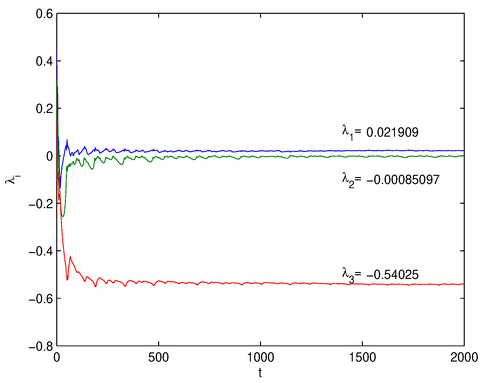
In this subsection, we calculate the Lyapunov exponents. The Lyapunov exponents for a discrete n-dimensional systems is given in [14], with the following definition. For other techniques of mathematics agains cancer see for instance [15,16,17]:
Definition 1.
Consider the n-dimensional discrete dynamical system:
where
is the vector field associated with map (15), let be its Jacobian evaluated at v, also define the matrix: .
Moreover, let be the modulus of the eigenvalue of the matrix where and .
Now, the Lyapunov exponents of n-dimensional discrete time models are defined by: .
7. Conclusions
This paper contributes to the study of the discrete cancer system with numerical and theoretical methods. As a result of this study, it is clearly understood that the Runge–Kutta method is the best method for discretization of the cancer system. Moreover, the Taylor series expansion method has good accuracy. The Euler discretization method is less accurate but easy to perform. The simulation plots suggest that the cancer system and simulation study reveal that dynamical patterns of the cancer system are dependent on the initial parametric values of the system variables, See Figure 1, Figure 2, Figure 3, Figure 4, Figure 5, Figure 6, Figure 7, Figure 8, Figure 9, Figure 10, Figure 11, Figure 12 and Figure 13. Hence, to obtain the system prediction of a cancer system, accurate quantification of the parametric values of different variables is important. This study could help biologists understand and appreciate the essence of measurement accuracy in different biological experiments and the power of inference through experiments.
In future work, we will study the control of chaos in this cancer system and generalize this system to the fourth-dimension.
Author Contributions
Conceptualization, T.S. and J.L.G.G.; methodology, K.D.; software, H.H.A.; writing—original draft preparation, M.S.A. All authors have read and agreed to the published version of the manuscript.
Funding
This research work was funded by Institutional Fund Projects under grant no. (IFPHI-228-130-2020). Therefore, authors gratefully acknowledge technical and financial support from the Ministry of Education and King Abdulaziz University, DSR, Jeddah, Saudi Arabia.
Data Availability Statement
Not applicable.
Conflicts of Interest
The authors declare no conflict of interest.
References
- De Pillis, L.G.; Radunskaya, A. The dynamics of an optimally controlled tumor model: A case study. Math. Comput. 2003, 37, 1221–1244. [Google Scholar] [CrossRef]
- De Pillis, L.G.; Radunskaya, A.E.; Wiseman, C.L. A validated mathematical model of cell-mediated immune response to tumor growth. Cancer Res. 2005, 65, 7950–7958. [Google Scholar] [CrossRef] [PubMed] [Green Version]
- Eftimie, R.; Macnamara, C.K.; Dushoff, J.; Bramson, J.L.; Earn, D.J. Bifurcations and chaotic dynamics in a tumour-immune-virus system. Math. Model. Nat. 2016, 11, 65–85. [Google Scholar] [CrossRef] [Green Version]
- Kamel, D. Dynamics in a Discrete-Time Three Dimensional Cancer System. Int. J. Appl. Math. 2019, 49, 1–7. [Google Scholar]
- Karakaya, B.; Turk, M.A.; Turk, M.; Gulten, A. Selection of optimal numerical method for implementation of Lorenz Chaotic system on FPGA. Int. Res. Eng. J. 2018, 2, 147–152. [Google Scholar]
- Sarif Hassan, S. Computational Complex Dynamics Of The Discrete Lorenz System. arXiv 2016, arXiv:1604.02671. [Google Scholar]
- Selvam, A.G.; Roslin, D.; Rajendran, J. A discrete model of Rössler system. Int. J. Adv. Technol. Eng. Sci. 2014, 2, 130–134. [Google Scholar]
- Yuksel, G.; Isik, O.R. Numerical analysis of Backward-Euler discretization for simplified magnetohydrodynamic flows. Appl. Math. Model. 2015, 39, 1889–1898. [Google Scholar] [CrossRef]
- Song, W.; Liang, J. Difference equation of Lorenz system. Int. J. Pure Appl. Math. 2013, 83, 101–110. [Google Scholar]
- Zwarycz-Makles, K.; Majorkowska-Mech, D. Gear and Runge-Kutta Numerical Discretization Methods in Differential Equations of Adsorption in Adsorption Heat Pump. Appl. Sci. 2018, 8, 2437. [Google Scholar] [CrossRef] [Green Version]
- Murray, J.D. Mathematical biology I: An introduction. In Interdisciplinary Applied Mathematics, 3rd ed.; Springer: New York, NY, USA, 2002. [Google Scholar]
- Shi, Y.; Chen, G. Chaos of discrete dynamical systems in complete metric spaces. Chaos Solitons Fractals 2004, 22, 555–571. [Google Scholar] [CrossRef]
- Shi, Y.; Chen, G. Discrete chaos in Banach spaces. Sci. China Ser. A Math. 2005, 48, 222–238. [Google Scholar] [CrossRef]
- Wolf, A.; Swift, J.B.; Swinney, H.L.; Vastano, J.A. Determining Lyapunov exponents from a time series. Phys. D Nonlinear Phenom. 1985, 16, 285–317. [Google Scholar] [CrossRef] [Green Version]
- Pérez-García, V.M.; Fitzpatrick, S.; Pérez-Romasanta, L.A.; Pesic, M.; Schucht, P.; Arana, E.; Sánchez-Gómez, P. Applied mathematics and nonlinear sciences in the war on cancer. Appl. Math. Nonlinear Sci. 2016, 1, 423–436. [Google Scholar] [CrossRef] [Green Version]
- De Anda-Jáuregui, G.; Fresno, C.; García-Cortés, D.; Enríquez, J.E.; Hernández-Lemus, E. Intrachromosomal regulation decay in breast cancer. Appl. Math. Nonlinear Sci. 2019, 4, 223–230. [Google Scholar] [CrossRef] [Green Version]
- Amer, A.; Nagah, A.; Osman, M.A.-R.E.-N.; Majid, A. Modeling the pathway of breast cancer in the Middle East. Appl. Math. Nonlinear Sci. 2022. ahead of print. [Google Scholar] [CrossRef]
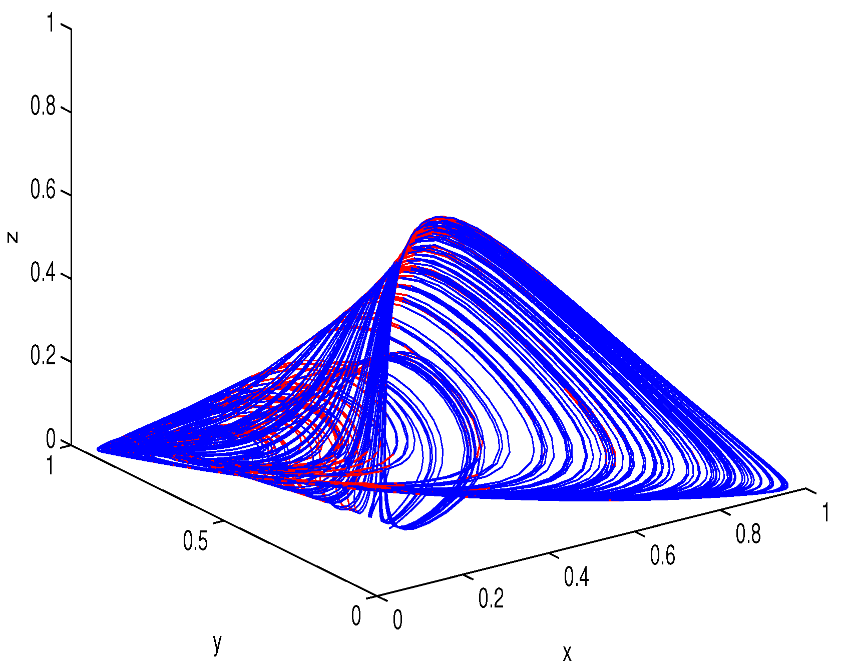
Figure 1.
Cancer attractor with , and parameter values .

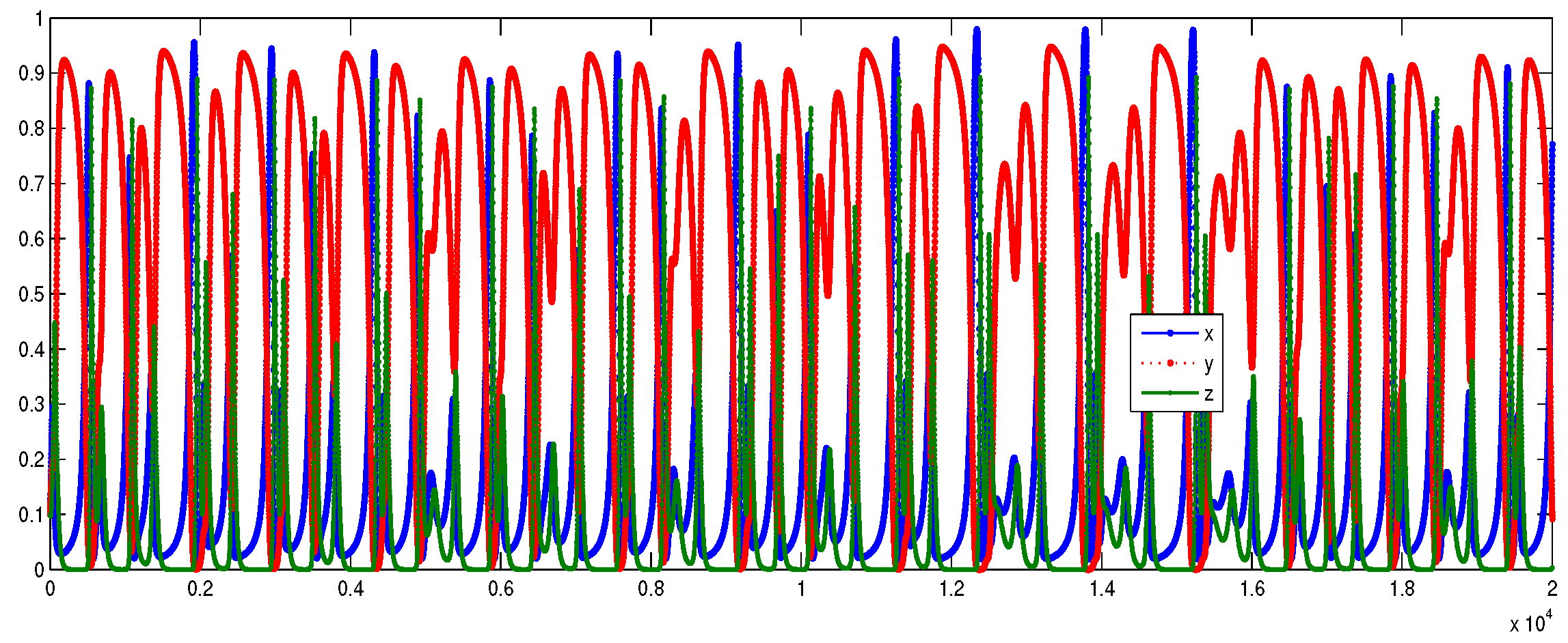
Figure 2.
The time series for system (2) with , and parameter values .
Figure 2.
The time series for system (2) with , and parameter values .

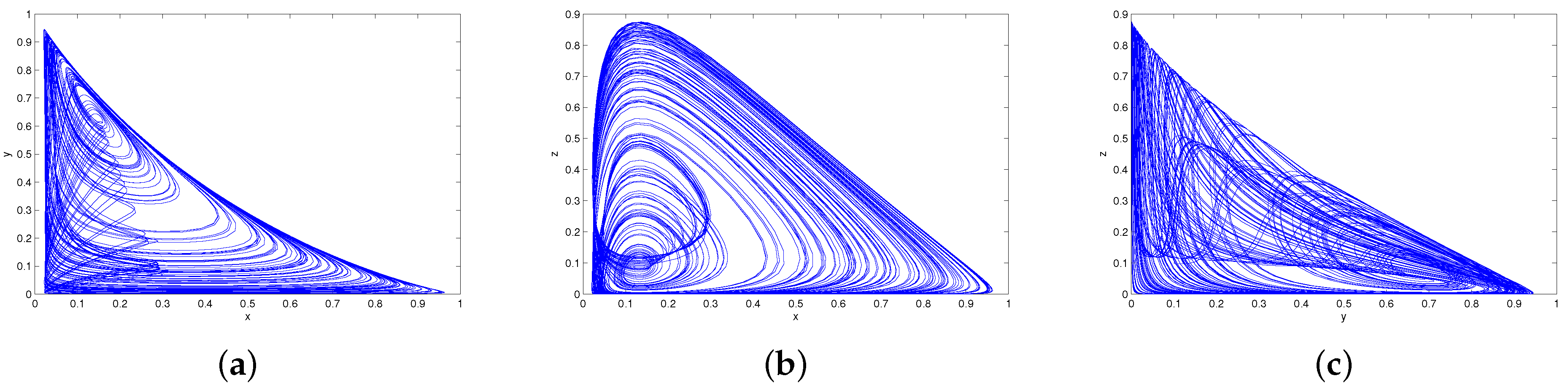
Figure 3.
Two-dimensional projections of the phase portraits onto the by each variable, , and z. (a) Normal cells : . (b) Effector immune cells : . (c) Tumor cells : .
Figure 3.
Two-dimensional projections of the phase portraits onto the by each variable, , and z. (a) Normal cells : . (b) Effector immune cells : . (c) Tumor cells : .

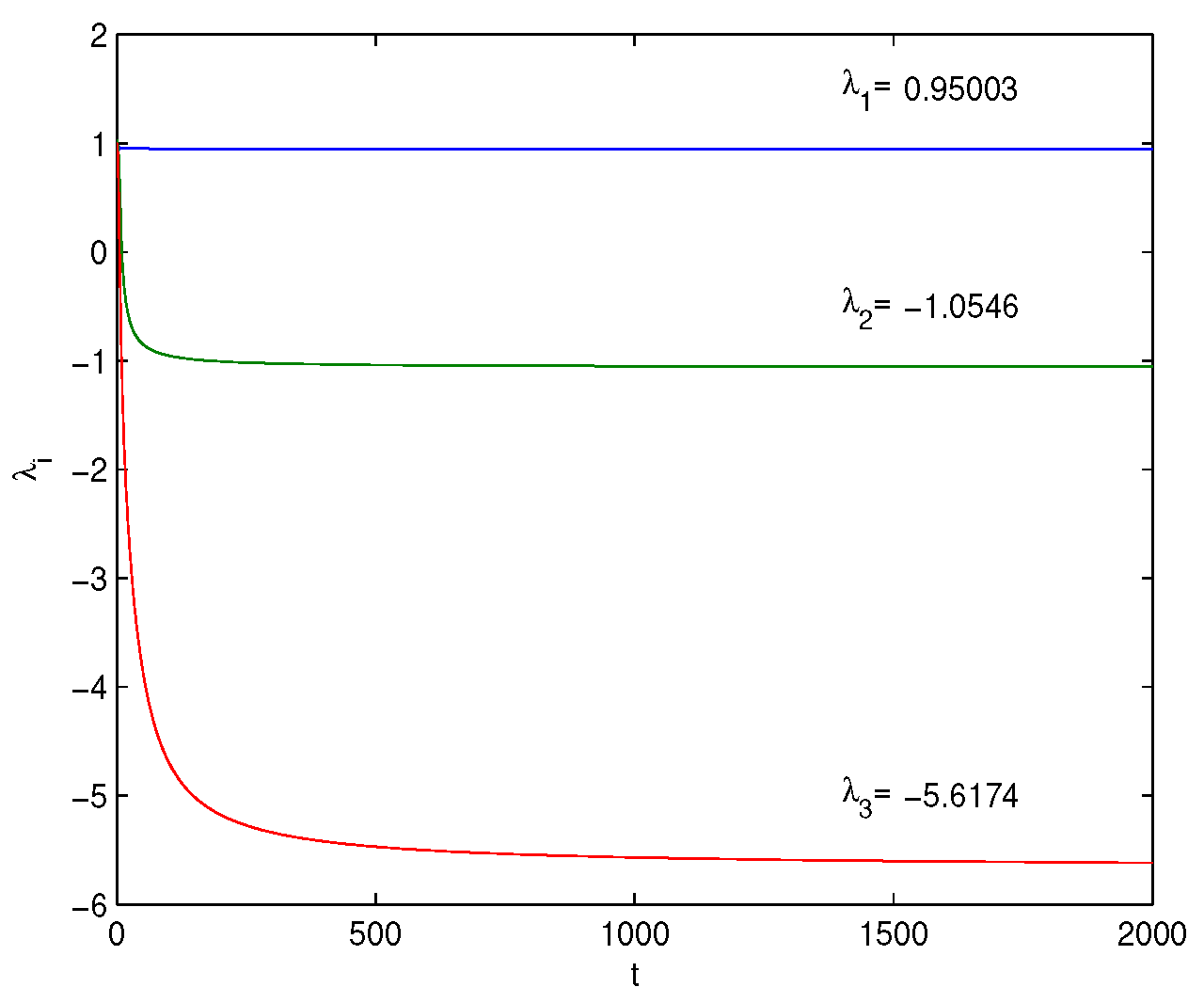
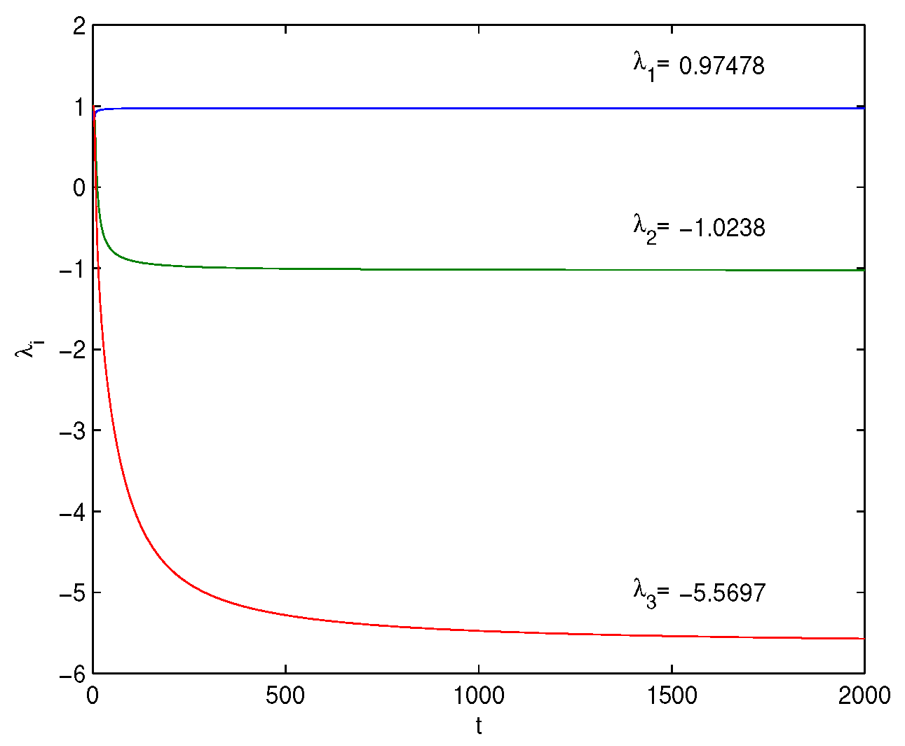
Figure 4.
The Lyapunov exponents of system (2) with , and parameter values .
Figure 4.
The Lyapunov exponents of system (2) with , and parameter values .

Figure 5.
Discrete cancer system attractor with the Euler method. (a) ; (b) .

Figure 6.
Projection of the attractor to system (1) onto the planes by each variable and z. (a) Host cells: ; (b) immune effector cells: ; (c) tumor cells: .
Figure 6.
Projection of the attractor to system (1) onto the planes by each variable and z. (a) Host cells: ; (b) immune effector cells: ; (c) tumor cells: .


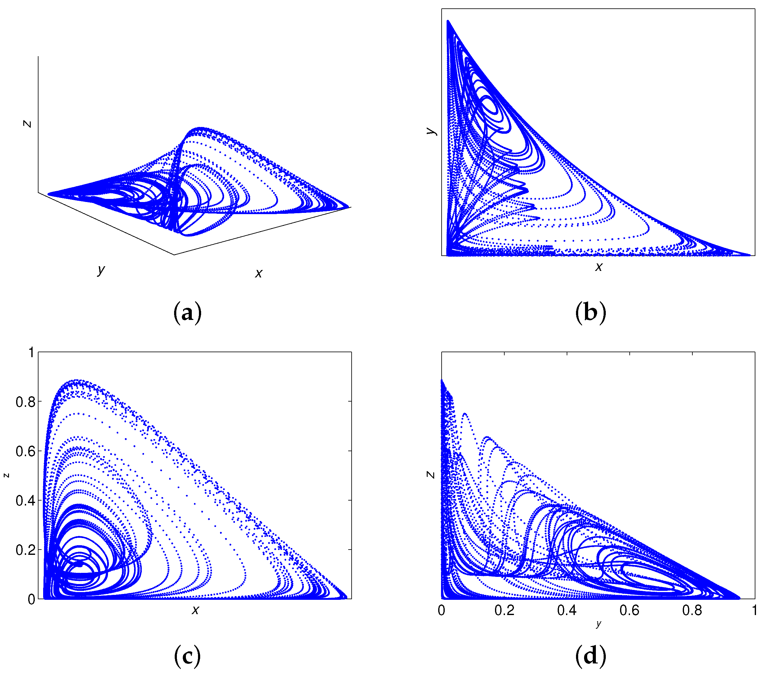
Figure 9.
(a) Strange attractor of system (6) with the Taylor method and . (b–d) Projection of the attractor to system (6) onto the planes by each variable , and z. (a) Strange attractor; (b) host cells: ; (c) immune effector cells: ; (d) tumor cells: .

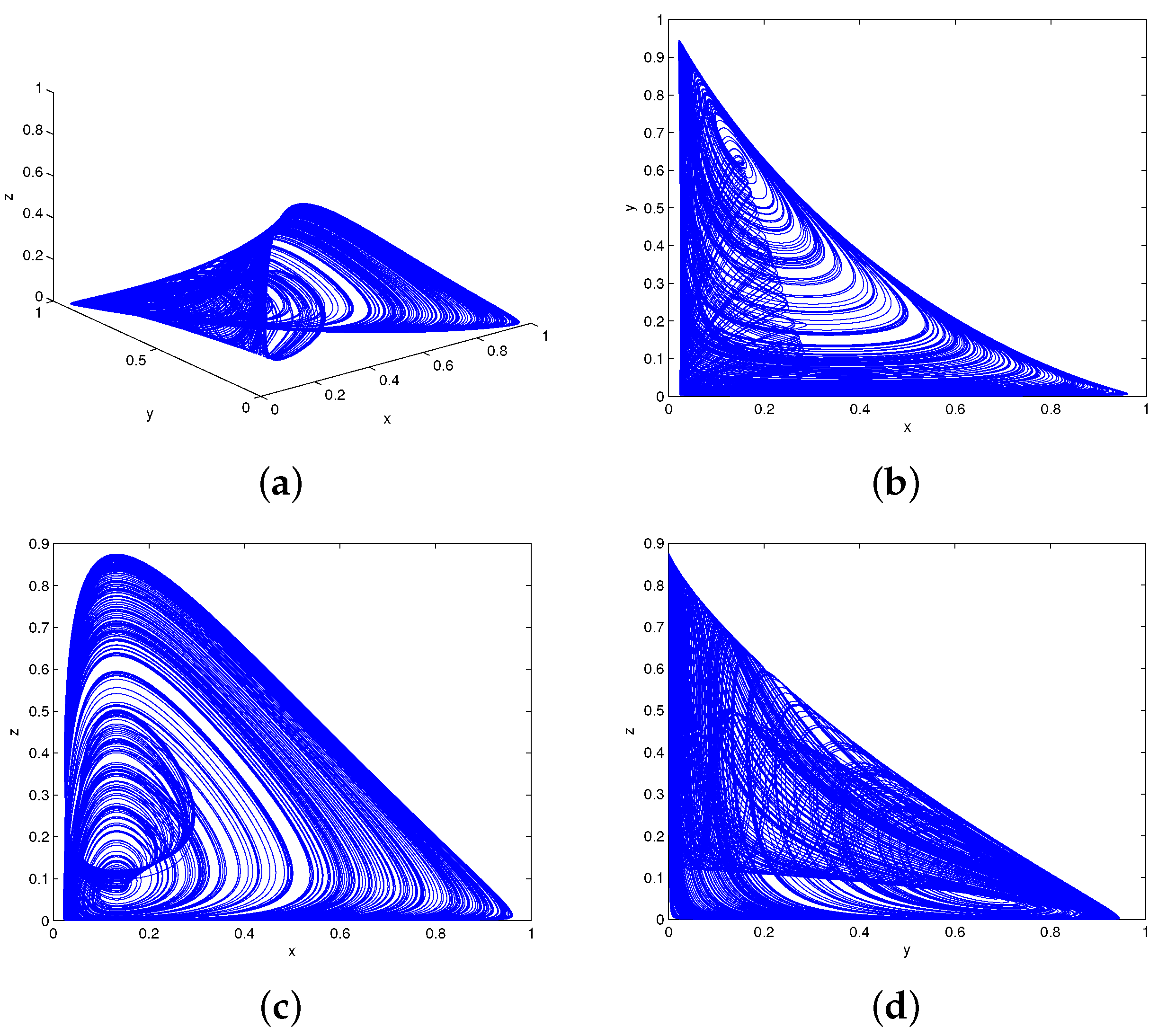
Figure 10.
(a) Strange attractor of system (8) with Runge-Kutta fourth order method and . (b–d) Projection of the attractor to system (8) onto the planes by each variable, , and z. (a) Strange attractor; (b) host cells: ; (c) immune effector cells: ; (d) tumor cells: .


Publisher’s Note: MDPI stays neutral with regard to jurisdictional claims in published maps and institutional affiliations. |
© 2022 by the authors. Licensee MDPI, Basel, Switzerland. This article is an open access article distributed under the terms and conditions of the Creative Commons Attribution (CC BY) license (https://creativecommons.org/licenses/by/4.0/).
Share and Cite
MDPI and ACS Style
Saeed, T.; Djeddi, K.; Guirao, J.L.G.; Alsulami, H.H.; Alhodaly, M.S. A Discrete Dynamics Approach to a Tumor System. Mathematics 2022, 10, 1774. https://0-doi-org.brum.beds.ac.uk/10.3390/math10101774
AMA Style
Saeed T, Djeddi K, Guirao JLG, Alsulami HH, Alhodaly MS. A Discrete Dynamics Approach to a Tumor System. Mathematics. 2022; 10(10):1774. https://0-doi-org.brum.beds.ac.uk/10.3390/math10101774
Chicago/Turabian StyleSaeed, Tareq, Kamel Djeddi, Juan L. G. Guirao, Hamed H. Alsulami, and Mohammed Sh. Alhodaly. 2022. "A Discrete Dynamics Approach to a Tumor System" Mathematics 10, no. 10: 1774. https://0-doi-org.brum.beds.ac.uk/10.3390/math10101774
Note that from the first issue of 2016, this journal uses article numbers instead of page numbers. See further details here.