
Zeroing Neural Network Approaches Based on Direct and Indirect Methods for Solving the Yang–Baxter-like Matrix Equation

 ,
,  ,
,  , and
, and 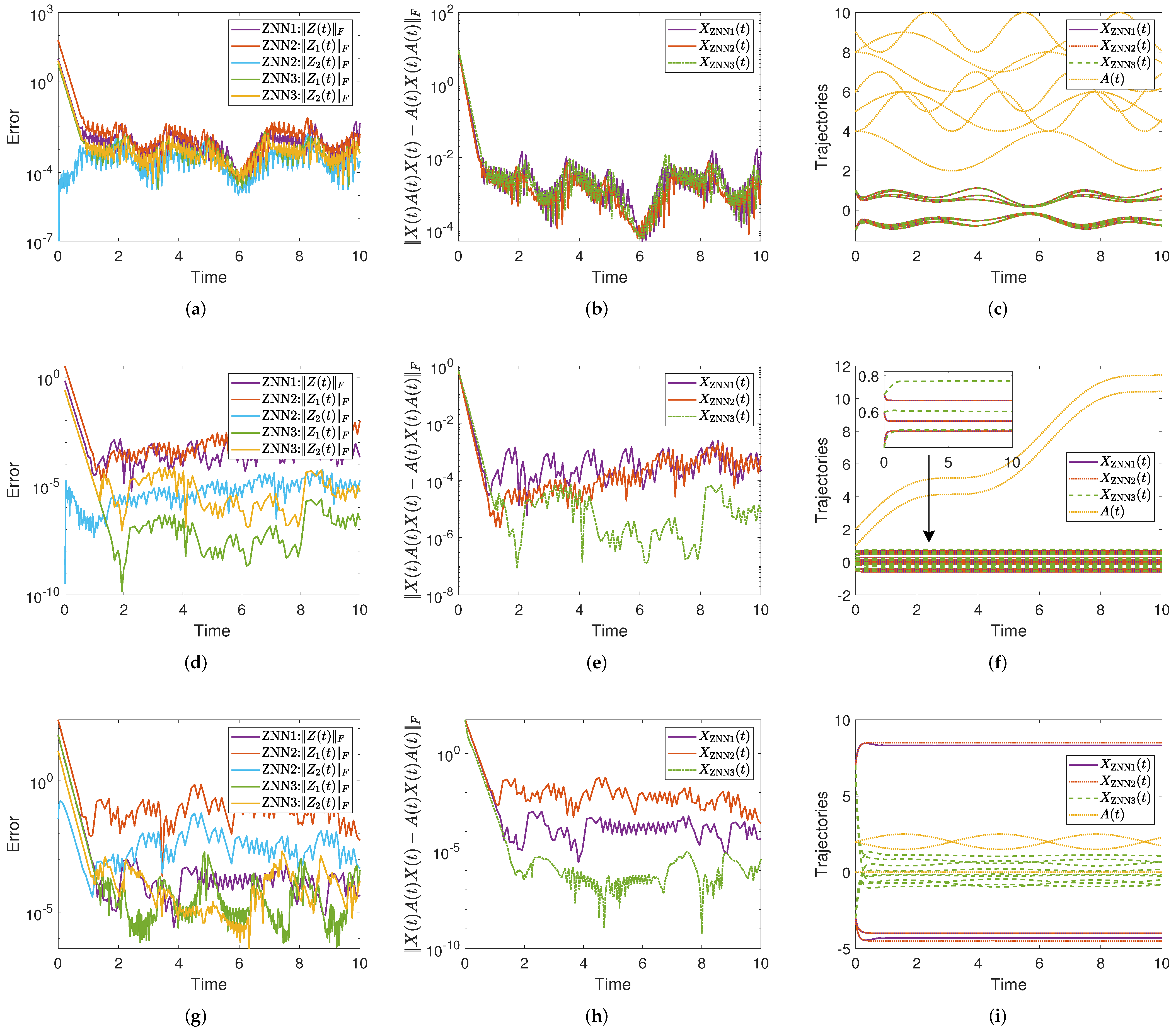
Abstract
:1. Introduction, Motivation, and Preliminaries
- Two novel ZNN models (ZNN2 and ZNN3) are introduced based on principles to find indirect numerical solutions to the TV-YBLME for an arbitrary input real TV matrix.
- Application of the Tikhonov regularization enables usability of the proposed dynamical systems in solving the TV-YBLME with the arbitrary (regular or singular) input real TV matrix.
- In particular, the ZNN model from [7] (ZNN1), based on a straightforward error matrix corresponding to the TV-YBLME, is extended to an arbitrary input real TV matrix using the Tikhonov principle.
- Four numerical experiments, including nonsingular and singular input matrices, are presented to confirm the efficiency of the proposed dynamics in addressing the TV-YBLME solving.
2. ZNN Model Based on Direct Solution to the TV-YBLME
3. ZNN Models Based on Indirect Methods for Solving the TV-YBLME
3.1. ZNN Model Based on Splitting the TV-YBLME
3.2. ZNN Model Based on Sufficient Conditions for a Solution
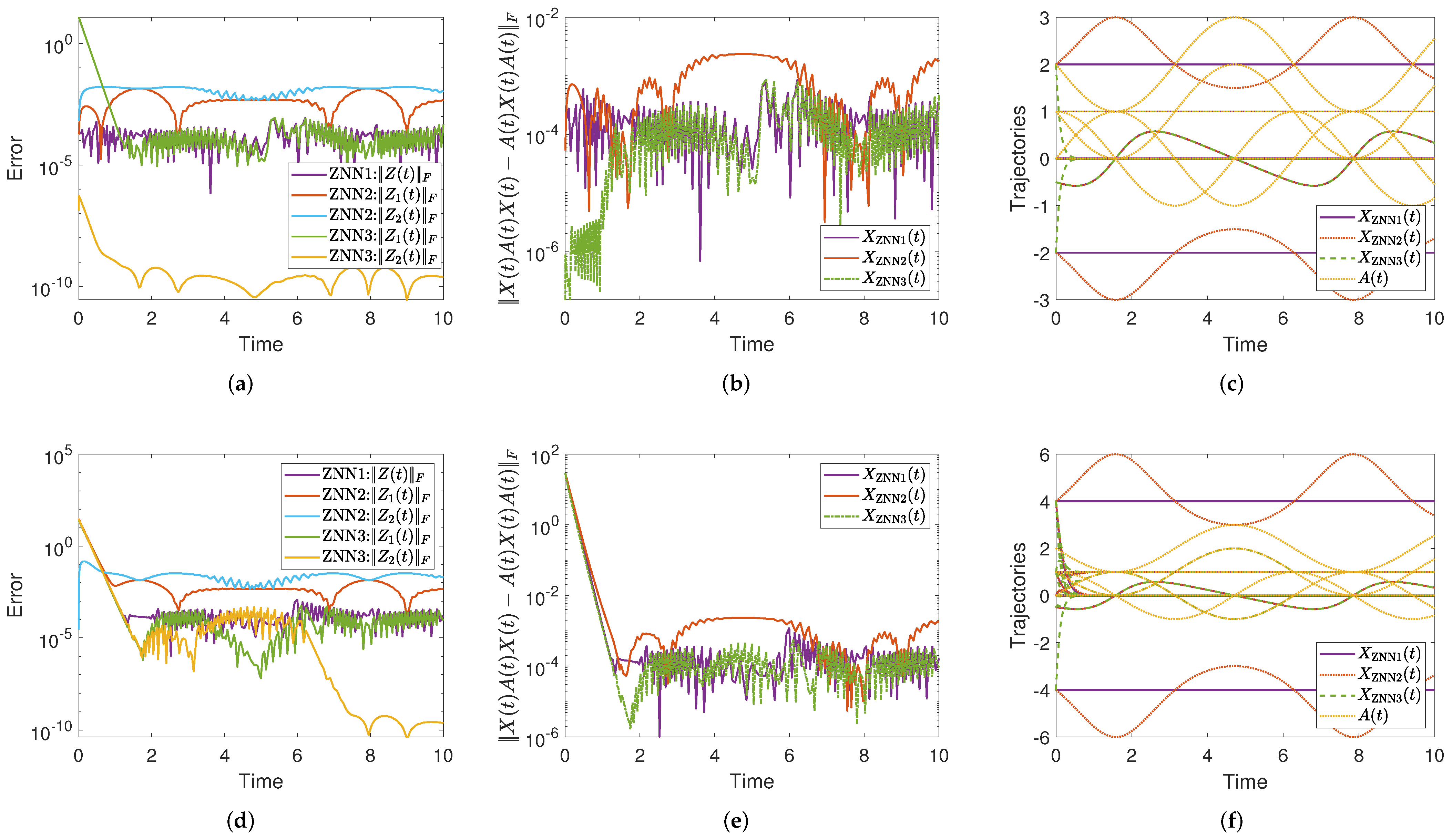
4. Simulation Results
4.1. Experiment 1
4.2. Experiment 2
4.3. Experiment 3
4.4. Experiment 4
4.5. Numerical Experiments Analysis—Findings and Comparison
5. Conclusions
- Since all types of noise significantly impact the ZNN model accuracies, noise sensitivity is a shortcoming of the proposed ZNN1, ZNN2, and ZNN3 models. As a result, future studies might concentrate on adapting the ZNN1, ZNN2, and ZNN3 models to a noise-handling ZNN dynamical system class. Such research will be a continuation of [27] from the constant matrix case to the time-varying case and from the direct ZNN model to various ZNN models.
- One could expect that further developments of ZNN evolutions (arising from different properties of solutions to the Yang–Baxter equation) will be possible.
Author Contributions
Funding
Institutional Review Board Statement
Informed Consent Statement
Data Availability Statement
Conflicts of Interest
References
- Yang, C.N. Some exact results for the many-body problem in one dimension with repulsive delta-function interaction. Phys. Rev. Lett. 1967, 19, 1312–1315. [Google Scholar] [CrossRef]
- Baxter, R.J. Partition function of the eight-vertex lattice model. Ann. Phys. 1972, 70, 193–228. [Google Scholar] [CrossRef]
- Matsumoto, D.K.; Shibukawa, Y. Quantum Yang-Baxter equation, braided semigroups, and dynamical Yang-Baxter maps. Tokyo J. Math. 2015, 38, 227–237. [Google Scholar] [CrossRef]
- Przytycki, J.H. Knot theory: From Fox 3-colorings of links to Yang-Baxter homology and Khovanov homology. In Knots, Low-Dimensional Topology and Applications; Springer: Cham, Switzerland, 2019; Volume 284, pp. 115–145. [Google Scholar] [CrossRef] [Green Version]
- Vieira, R.S.; Lima-Santos, A. Solutions of the Yang-Baxter equation for (n + 1) (2n + 1)-vertex models using a differential approach. J. Stat. Mech. 2021, 2021, 053103. [Google Scholar] [CrossRef]
- Tsuboi, Z. Quantum groups, Yang-Baxter maps and quasi-determinants. Nucl. Phys. B 2018, 926, 200–238. [Google Scholar] [CrossRef]
- Zhang, H.; Wan, L. Zeroing neural network methods for solving the Yang-Baxter-like matrix equation. Neurocomputing 2020, 383, 409–418. [Google Scholar] [CrossRef]
- Kumar, A.; Cardoso, J.R.; Singh, G. Explicit solutions of the singular Yang-Baxter-like matrix equation and their numerical computation. Mediterr. J. Math. 2022, 19, 85. [Google Scholar] [CrossRef]
- Ding, J.; Zhang, C.; Rhee, N.H. Further solutions of a Yang-Baxter-like matrix equation. East Asian J. Appl. Math. 2013, 3, 352–362. [Google Scholar] [CrossRef]
- Zhang, Y.; Ge, S.S. Design and analysis of a general recurrent neural network model for time-varying matrix inversion. IEEE Trans. Neural Netw. 2005, 16, 1477–1490. [Google Scholar] [CrossRef] [PubMed] [Green Version]
- Stanimirović, P.S.; Katsikis, V.N.; Zhang, Z.; Li, S.; Chen, J.; Zhou, M. Varying-parameter Zhang neural network for approximating some expressions involving outer inverses. Optim. Methods Softw. 2020, 35, 1304–1330. [Google Scholar] [CrossRef]
- Kornilova, M.; Kovalnogov, V.; Fedorov, R.; Zamaleev, M.; Katsikis, V.N.; Mourtas, S.D.; Simos, T.E. Zeroing neural network for pseudoinversion of an arbitrary time-varying matrix based on singular value decomposition. Mathematics 2022, 10, 1208. [Google Scholar] [CrossRef]
- Simos, T.E.; Katsikis, V.N.; Mourtas, S.D.; Stanimirović, P.S.; Gerontitis, D. A higher-order zeroing neural network for pseudoinversion of an arbitrary time-varying matrix with applications to mobile object localization. Inf. Sci. 2022, 600, 226–238. [Google Scholar] [CrossRef]
- Stanimirović, P.S.; Katsikis, V.N.; Li, S. Integration enhanced and noise tolerant ZNN for computing various expressions involving outer inverses. Neurocomputing 2019, 329, 129–143. [Google Scholar] [CrossRef]
- Katsikis, V.N.; Mourtas, S.D.; Stanimirović, P.S.; Zhang, Y. Solving complex-valued time-varying linear matrix equations via QR decomposition with applications to robotic motion tracking and on angle-of-arrival localization. IEEE Trans. Neural Netw. Learn. Syst. 2021, 1–10. [Google Scholar] [CrossRef]
- Ma, H.; Li, N.; Stanimirović, P.S.; Katsikis, V.N. Perturbation theory for Moore–Penrose inverse of tensor via Einstein product. Comput. Appl. Math. 2019, 38, 111. [Google Scholar] [CrossRef]
- Katsikis, V.N.; Mourtas, S.D.; Stanimirović, P.S.; Li, S.; Cao, X. Time-varying mean-variance portfolio selection problem solving via LVI-PDNN. Comput. Oper. Res. 2022, 138, 105582. [Google Scholar] [CrossRef]
- Stanimirović, P.S.; Katsikis, V.N.; Li, S. Hybrid GNN-ZNN models for solving linear matrix equations. Neurocomputing 2018, 316, 124–134. [Google Scholar] [CrossRef]
- Katsikis, V.N.; Stanimirović, P.S.; Mourtas, S.D.; Li, S.; Cao, X. Generalized Inverses: Algorithms and Applications; Mathematics Research Developments; Chapter Towards Higher Order Dynamical Systems; Nova Science Publishers, Inc.: Hauppauge, NY, USA, 2021; pp. 207–239. [Google Scholar]
- Katsikis, V.N.; Mourtas, S.D.; Stanimirović, P.S.; Zhang, Y. Continuous-time varying complex QR decomposition via zeroing neural dynamics. Neural Process. Lett. 2021, 53, 3573–3590. [Google Scholar] [CrossRef]
- Zhang, Y.; Guo, D. Zhang Functions and Various Models; Springer: Berlin/Heidelberg, Germany, 2015. [Google Scholar] [CrossRef]
- Khalaf, G.; Shukur, G. Choosing ridge parameter for regression problems. Commun. Stat. Theory Methods 2005, 34, 1177–1182. [Google Scholar] [CrossRef]
- Dai, J.; Chen, Y.; Xiao, L.; Jia, L.; He, Y. Design and analysis of a hybrid GNN-ZNN model with a fuzzy adaptive factor for matrix inversion. IEEE Trans. Ind. Inform. 2022, 18, 2434–2442. [Google Scholar] [CrossRef]
- Jia, L.; Xiao, L.; Dai, J.; Cao, Y. A novel fuzzy-power zeroing neural network model for time-variant matrix Moore-Penrose inversion with guaranteed performance. IEEE Trans. Fuzzy Syst. 2021, 29, 2603–2611. [Google Scholar] [CrossRef]
- Jia, L.; Xiao, L.; Dai, J.; Qi, Z.; Zhang, Z.; Zhang, Y. Design and application of an adaptive fuzzy control strategy to zeroing neural network for solving time-variant QP problem. IEEE Trans. Fuzzy Syst. 2021, 29, 1544–1555. [Google Scholar] [CrossRef]
- Katsikis, V.N.; Stanimirović, P.S.; Mourtas, S.; Xiao, L.; Karabašević, D.; Stanujkić, D. Zeroing Neural Network with fuzzy parameter for computing pseudoinverse of arbitrary matrix. IEEE Trans. Fuzzy Syst. 2021, 1. [Google Scholar] [CrossRef]
- Shi, T.; Tian, Y.; Sun, Z.; Liu, K.; Jin, L.; Yu, J. Noise-tolerant neural algorithm for online solving Yang–Baxter-type matrix equation in the presence of noises: A control-based method. Neurocomputing 2021, 424, 84–96. [Google Scholar] [CrossRef]


Publisher’s Note: MDPI stays neutral with regard to jurisdictional claims in published maps and institutional affiliations. |
© 2022 by the authors. Licensee MDPI, Basel, Switzerland. This article is an open access article distributed under the terms and conditions of the Creative Commons Attribution (CC BY) license (https://creativecommons.org/licenses/by/4.0/).
Share and Cite
Jiang, W.; Lin, C.-L.; Katsikis, V.N.; Mourtas, S.D.; Stanimirović, P.S.; Simos, T.E. Zeroing Neural Network Approaches Based on Direct and Indirect Methods for Solving the Yang–Baxter-like Matrix Equation. Mathematics 2022, 10, 1950. https://0-doi-org.brum.beds.ac.uk/10.3390/math10111950
Jiang W, Lin C-L, Katsikis VN, Mourtas SD, Stanimirović PS, Simos TE. Zeroing Neural Network Approaches Based on Direct and Indirect Methods for Solving the Yang–Baxter-like Matrix Equation. Mathematics. 2022; 10(11):1950. https://0-doi-org.brum.beds.ac.uk/10.3390/math10111950
Chicago/Turabian StyleJiang, Wendong, Chia-Liang Lin, Vasilios N. Katsikis, Spyridon D. Mourtas, Predrag S. Stanimirović, and Theodore E. Simos. 2022. "Zeroing Neural Network Approaches Based on Direct and Indirect Methods for Solving the Yang–Baxter-like Matrix Equation" Mathematics 10, no. 11: 1950. https://0-doi-org.brum.beds.ac.uk/10.3390/math10111950