Numerical Construction of Viable Sets for Autonomous Conflict Control Systems

Abstract

A conflict control system with state constraints is under consideration. A method for finding viability kernels (the largest subsets of state constraints where the system can be confined) is proposed. The method is related to differential games theory essentially developed by N. N. Krasovskii and A. I. Subbotin. The viability kernel is constructed as the limit of sets generated by a Pontryagin-like backward procedure. This method is implemented in the framework of a level set technique based on the computation of limiting viscosity solutions of an appropriate Hamilton–Jacobi equation. To fulfill this, the authors adapt their numerical methods formerly developed for solving time-dependent Hamilton–Jacobi equations arising from problems with state constraints. Examples of computing viability sets are given.

1. Introduction

In many technical control problems, it is necessary to keep a controlled system within prescribed state constraints in the presence of disturbances. Such a control process is usually considered on a large (infinite) time interval, and no performance index is used. One approach to such problems is given by robust control theory [1] based on the methods of stability theory. Viability theory [2] can be considered as an alternative approach. Namely, a viable subset of the state constraint determines a feedback strategy that can keep the state vector within this subset. One can design such a feedback strategy, using the extremal aiming procedure described in [3]. A method for constructing the viability kernel (the maximal viable subset of the state constraint) is proposed in [4]. This method is based on the necessary and sufficient viability conditions formulated in terms of contingent cones. The book [5] considers a wide range of questions related to the analysis and construction of viability sets. A procedure for constructing viability kernels for control systems (without any conflict controls) is proposed in [6].

The present paper extends the short communication [7] and the report [8]. A constructive method for finding viability kernels is described and theoretically analyzed. The approach used is related to the theory of differential games (see [3,9]). The viability kernel is constructed as the limit of sets generated by a Pontryagin-like backward procedure (see [9]). The idea of such a passage to the limit was proposed in [10] for linear systems with discrete time. In the paper presented, an approximation scheme for finding the solvability kernel for a general class of nonlinear autonomous controlled system is proposed. This algorithm is numerically implemented in terms of level sets. The idea consists in the computation of the limit in the time of viscosity solutions (see [11,12]) of an appropriate Hamilton–Jacobi equation. To implement this idea, the authors adapt their numerical methods formerly developed for solving time-dependent Hamilton–Jacobi equations arising from problems with state constraints. Examples of computing viability sets are given.

2. Differential Game and Viability Kernels

Consider a differential game with the autonomous dynamics:

$$\dot{x}=f(x,u,v),x\in R^n,u\in P\subset R^p,v\in Q\subset R^q$$

(1)

Here, x is the state vector, u and v are control parameters of the first and second players, respectively, and P and Q are compacts of the corresponding dimensions. We suppose that f satisfies standard requirements: continuity in $x,u$ and v; the Lipschitz condition in x; and a growth condition that provides the continuability of the solutions to any time interval.

Based on the conflict control system (1), consider for any $v\in Q$ the differential inclusion:

$$\dot{x}\in F_v\left(x\right)=\overline{co}\left\{f(x,P,v)\right\}$$

(2)

Definition 1 (u-stability property [3]). Let T be an arbitrary time instant. A set $W\subset (-\infty ,T]\times R^n$ is said to be $u-$stable on the interval $(-\infty ,T]$ if for any initial position, $(t_{*},x_{*})\in W$, for any time instant, $t^{*}(t_{*}\le t^{*}\le T)$, for any $v\in Q$, there exists a solution, $x(·)$, to the differential inclusion (2) with the initial state $x\left(t_{*}\right)=x_{*}$, such that $(t^{*},x\left(t^{*}\right))\in W$.

Definition 2 (viability property [2]). A set $K\subset R^n$ is said to be viable if for any $x_{*}\in K$, for any $v\in Q$ there exists a solution $x(·)$ to the differential inclusion (2) with the initial state $x\left(0\right)=x_{*}$ such that $x\left(t\right)\in K,t\ge 0$.

Definition 3 (viability kernel [2]). For a given compact set $G\subset R^n$ denote by $Viab\left(G\right)$ the largest subset of G with the viability property. This subset is called the viability kernel of G.

The following assertions follow from Definitions 1–3:

(1)

The closure of a u-stable (viable) set is a u-stable (viable) set.

(2)

The union of any family of u-stable (viable) sets is a u-stable (viable) set.

(3)

If $W\subset (-\infty ,T]\times R^n$ is a u-stable closed set, then for any initial position, $(t_{*},x_{*})\in W$, for any $v\in Q$, there exists a solution, $x(·)$, to the differential inclusion (2) with the initial state $x\left(t_{*}\right)=x_{*}$ such that $(t,x\left(t\right))\in W,t_{*}\le t\le T.$

The first assertion follows from the compactness and semi-continuity of solution sets of differential inclusions; see e.g., [13], and notice that the solution set of Equation (2) depends, even Lipschitz continuous, on the initial state. The second assertion follows from the definition of u-stability (viability). The third assertion can be proven by considering ever finer subdivisions of the interval $[t_{*},T]$, step-by-step constructing solutions of Equation (2) that satisfy the assertion at nodes of the subdivisions and using the compactness of the solution sets of Equation (2).

Assertion (3) shows that Definition 2 is a special case of Definition 1 with $T=\infty$ and $W=R\times K$. Assertions (1) and (2) provide the existence of the viability kernel, $Viab\left(G\right)$, for any compact set, G, if there exists at least one viable subset of G. Thus, the following problem can be considered.

Problem. Given a compact set $G\subset R^n$ it is required to construct the viability kernel, $Viab\left(G\right)$.

To solve this problem, fix an arbitrary $T\in R$ and introduce the set $N=(-\infty ,T]\times G$. Due to Assertions (1) and (2), there exists a closed maximal u-stable on the interval $(-\infty ,T]$ set $W\subset N$. For any time instant, $t\le T$, denote

$$W\left(t\right)=\{x\in R^n:(t,x)\in W\}$$

Remark 1. The family $\left\{W\right(t):t\le T\}$ has the property of monotonicity: $W\left(t_1\right)\subset W\left(t_2\right)$ for $t_1\le t_2\le T$. Really, if $\mathcal{W}$ is a u-stable set, then the set $\widehat{\mathcal{W}}$ defined by the cross-sections $\widehat{\mathcal{W}}\left(t\right)={\cup }_{\tau \le t}\mathcal{W}\left(\tau \right)$ is also u-stable. Therefore, the maximal u-stable set, W, must have the required monotonicity property.

These facts immediately follow from the above definitions, and they are left to the reader to prove.

Proposition 1. Let ${\left\{X_i\right\}}_{i=0}^{\infty }$ be a sequence of nonempty compact sets such that $X_j\subset X_i$ if $j>i$, and let $X={\bigcap }_{i=0}^{\infty }{X}_i$, then $X\ne Ø$ and $X_i$ $converge$ to X in the $Hausdorffmetric.$

Proof. First, X is nonempty as the intersection of embedded compacts. Second, assume that the convergence is absent. Then, there exists an $ϵ>0$, such that $A_k:=X_k\bigcap \text{cl}(X_0^{ϵ}\setminus X^{ϵ})\ne Ø$ for all $k\ge 0$. Here, the upper index, $ϵ$, denotes the $ϵ$-neighborhood of sets, and the symbol “cl” denotes the closure operation. The sets $A_k,k\ge 0$, are compact and embedded. Therefore, there exists $x\in {\bigcap }_{k\ge 0}{A}_k=X\bigcap \text{cl}(X_0^{ϵ}\setminus X^{ϵ})$, which is a contradiction. ☐

Theorem 1. If $W\left(t\right)\ne Ø$ for any $t\le T$, then there exists the Hausdorff limit $\underset{t\to -\infty }{lim}W\left(t\right)$ and:

$$\underset{t\to -\infty }{lim}W\left(t\right)=\bigcap _{t\le T}W\left(t\right)=Viab\left(G\right)\ne \varnothing$$

Otherwise, there is not any viable subset of G.

Proof. Denote $K:={\bigcap }_{t\le T}W\left(t\right)$ for brevity. If for any $t\le T$, the set, $W\left(t\right)$, is nonempty, then K is also nonempty as the intersection of nonempty embedded compacts. Show that K is viable in the sense of Definition 2. Choose arbitrary $x_{*}\in K,v\in Q$ and $\delta >0$. By Proposition 1, for any $\epsilon >0$, there exists $t_{\epsilon }$, such that:

$$K\subset W\left(t\right)\subset K^{\epsilon },for allt\le t_{\epsilon }$$

(3)

The condition, $x_{*}\in K$, implies the inclusion, $x_{*}\in W(t_{\epsilon }-\delta )$. By virtue of u-stability of the set W, there exists a solution, $x(·)$, of Equation (2) with the initial state $x(t_{\epsilon }-\delta )=x_{*}$, such that $x\left(t_{\epsilon }\right)\in W\left(t_{\epsilon }\right)$. With the autonomy of the differential inclusions (2), we conclude the existence of a solution, $x(·)$, of Equation (2), such that $x\left(0\right)=x_{*}$ and $x\left(\delta \right)\in K^{\epsilon }.$

Thus, for arbitrarily small $\epsilon >0$, there exists a solution, $x(·)$, of Equation (2) that satisfies the relations, $x\left(0\right)=x_{*}$ and $x\left(\delta \right)\in K^{\epsilon }$. Since the solution set of Equation (2) is compact, this gives a solution, $x(·)$, such that $x\left(0\right)=x_{*}$ and $x\left(\delta \right)\in K$. Thus, we have proven the viability property of K, and relation (3) proves the Hausdorff convergence of $W\left(t\right)$ to K as $t\to -\infty$.

Assume now that $K^{\prime }\subset G$ is a viable set, such that $K\subset K^{\prime }$. As was noticed in the comment to Definition 2, the viability property of $K^{\prime }$ means the u-stability property of the set $(-\infty ,T]\times K^{\prime }$. Since $(-\infty ,T]\times K^{\prime }\subset N$, and W is the maximal u-stable set belonging to N, then $(-\infty ,T]\times K^{\prime }\subset W$. Thus, $K^{\prime }\subset W\left(t\right)$ for all $t\le T$, and therefore, $K^{\prime }\subset {\bigcap }_{t\le T}W\left(t\right)=K$. This proves Theorem 1. ☐

3. Approximation

Immediate implementation of Theorem 1 for finding $Viab\left(G\right)$ requires precise computing of the sets $W\left(t\right)$ for $t\in (-\infty ,T]$. If, for example, the step-by-step backward procedure from [9] related to the dynamic programming method is used, then the computational error grows infinitely as $t\to -\infty .$ The algorithm proposed in the current paper uses the idea of decreasing the step of the backward procedure simultaneously with the passage to the limit as time goes to infinity. The algorithm looks as follows:

$$\begin{array}{ccc}\hfill K_0& =& G\hfill \\ \hfill K_{i+1}& =& \bigcap _{v\in Q}[\bigcup _{x\in K_i}(x-{\delta }_{i+1}{F}_v\left(x\right))+{\delta }_{i+1}^2\beta S]\bigcap G\hfill \end{array}$$

(4)

Here, S is the unit closed ball in $R^n,\beta =LM$, L is the Lipschitz constant of $F_v$, and $M=sup\left\{\right|f|:f\in F_v\left(x\right),x\in G,v\in Q\}.$

Theorem 2. Let the family $\left\{K_i\right\}$ be defined by Equation (4), where the sequence {${\delta }_i\}$ is such that ${\delta }_i\to 0$ and ${\sum }_{i=1}^{\infty }$ ${\delta }_i=\infty$. If $K_i\ne Ø$ for any $i>1$, then there exists the Hausdorff limit, ${lim}_{i\to \infty }{K}_i$, and

$$\underset{i\to \infty }{lim}{K}_i=Viab\left(G\right)\ne \varnothing$$

Otherwise, there is no viable subset of G.

Before starting the proof of Theorem 2, we prove three auxiliary lemmas. The first lemma shows a discrete u-stability of the family $\left\{K_i\right\}$ generated by Equation (4). Assume just for the simplicity of subsequent calculations that ${\delta }_{j}L\le 1$ for all $j>0$. This requirement allows us to avoid the consideration of terms of the form ${\sum }_{i=l+1}^s$ ${\delta }_i^3$ in the proof of Lemma 1, which reduces the amount of calculations.

Lemma 1. Let l and s be integers such that $0<l<s$. Let $v\in Q$ be fixed. If $x_{*}\in K_s$, then there exists a solution, $x(·)$, of Equation (2) with $x\left(0\right)=x_{*}$, such that $x\left(\sigma \right)\in K_l^{\omega }$, where $\sigma ={\sum }_{i=l+1}^s$ ${\delta }_i$, $\omega =4LM{e}^{L\sigma }{\sum }_{i=l+1}^s$ ${\delta }_i^2$.

We first prove the following two auxiliary propositions.

Proposition 2. Let $v\in Q$ and $x_1,x_2\in R^n$. If $|x_1-x_2|\le \alpha$, then for any solution, $x_1(·)$, of differential inclusion (2) with the initial state $x_1\left(0\right)=x_1$, there exists a solution, $x_2(·)$, with the initial state $x_2\left(0\right)=x_2$, such that $|x_1\left(t\right)-x_2\left(t\right)|\le \alpha e^{Lt}.$

Proof of Proposition 2. The proof immediately follows from the Filippov–Gronwall inequality obtained in [14], Theorem 1. ☐

Proposition 3. Let $v\in Q$, $j>0$ and $\alpha >0$ be fixed. If $x_0\in K_j^{\alpha }$, then there is a solution, $x(·)$, of Equation (2) with the initial condition $x\left(0\right)=x_0$, such that $x($ ${\delta }_j)\in K_{j-1}^{{\alpha }_1}$, where ${\alpha }_1=\alpha e^{L{\delta }_j}+4ML$ ${\delta }_j^2.$

Proof of Proposition 3. Choose $v\in Q,j>0$ and $\alpha >0$. Let $x_0\in K_j^{\alpha }$. Then, there exists a point, $x_{*}\in K_j$, satisfying $|x_0-x_{*}|\le \alpha$. By the definition of $K_j$, there are a point $\overline{x}\in K_{j-1}$ and vectors $\overline{g}\in F_v\left(\overline{x}\right)$ and $\overline{h}$, $|\overline{h}|\le 1$, such that:

$$x_{*}=\overline{x}-{\delta }_j\overline{g}+LM{\delta }_j^2\overline{h}\text{or}\overline{x}=x_{*}+{\delta }_j\overline{g}-LM{\delta }_j^2\overline{h}$$

Using the Lipschitz property of the right-hand side of Equation (2), choose a vector, $g_{*}\in F_v\left(x_{*}\right)$, to provide the inequality $|g_{*}-\overline{g}|\le L|x_{*}-\overline{x}|$. Denote $\widehat{x}=x_{*}+$ ${\delta }_j{g}_{*}$ and calculate:

$$|\widehat{x}-\overline{x}|\le {\delta }_j|g_{*}-\overline{g}|+LM{\delta }_j^2\le {\delta }_{j}L|x_{*}-\overline{x}|+LM{\delta }_j^2\le 2LM{\delta }_j^2+L^{2}M{\delta }_j^3$$

Accounting for the technical assumption ${\delta }_{j}L\le 1$, $j>0$, simplifies the last estimate as follows:

$$|\widehat{x}-\overline{x}|\le 3LM{\delta }_j^2$$

(5)

Let $g\left(x\right)\in F_v\left(x\right)$ be the nearest point to $g_{*}$ for every $x\in R^n$. Obviously, the function $x\to g\left(x\right)$ is continuous and satisfies the following inequality, due to the Lipschitz property of $F_v(·)$:

$$|g\left(x\right)-g_{*}|\le L|x-x_{*}|$$

(6)

Suppose $x(·)$ is a solution of the differential equation $\dot{x}=g\left(x\right)$ with the initial state $x\left(0\right)=x_{*}$. Then:

$$x\left({\delta }_j\right)-\widehat{x}={\int }_0^{{\delta }_j}(g\left(x\left(\xi \right)\right)-g_{*})d\xi$$

The last equation and the estimate (6) yield the inequality:

$$|x\left({\delta }_j\right)-\widehat{x}|\le {\delta }_{j}Lmax\left\{|x\left(\xi \right)-x_{*}|:\xi \in [0,{\delta }_j]\right\}\le {\delta }_j^{2}LM$$

and, with Equation (5), it holds that:

$$|\overline{x}-x\left({\delta }_j\right)|\le 4LM{\delta }_j^2$$

By Proposition 2, there exists a solution, $x_0(·)$, of Equation (2) with the initial state $x_0\left(0\right)=x_0$, such that:

$$|x_0({\delta }_j)-x({\delta }_j\left)\right|\le \alpha e^{L{\delta }_j}$$

Then:

$$|x_0\left({\delta }_j\right)-\overline{x}|\le \alpha e^{L{\delta }_j}+4LM{\delta }_j^2$$

and therefore:

$$x_0\left({\delta }_j\right)\in K_{j-1}^{{\alpha }_1},{\alpha }_1=\alpha e^{L{\delta }_j}+4LM{\delta }_j^2$$

Proposition 3 is proven. ☐

Proof of Lemma 1. Let $x_{*}\in K_s$ be chosen. Setting $D=4ML$ and applying Proposition 3, we construct a solution, $x(·)$, of Equation (2) that satisfies the conditions:

$$\begin{array}{c}x\left(0\right)=x_{*}\in K_s\hfill \\ x\left({\delta }_s\right)\in K_{s-1}^{{\alpha }_0},{\alpha }_0=D{\delta }_s^2\hfill \\ x({\delta }_s+{\delta }_{s-1})\in K_{s-2}^{{\alpha }_1},{\alpha }_1={\alpha }_0{e}^{L{\delta }_{s-1}}+D{\delta }_{s-1}^2\hfill \\ ...\hfill \\ x({\delta }_s+{\delta }_{s-1}+...+{\delta }_{l+1})\in K_l^{{\alpha }_p},{\alpha }_p={\alpha }_{p-1}{e}^{L{\delta }_{l+1}}+D{\delta }_{l+1}^2\hfill \end{array}$$

It is easy to estimate ${\alpha }_p$ to obtain the inequality:

$${\alpha }_p\le e^{L\sigma }D\sum _{i=l+1}^s{\delta }_i^2$$

where $\sigma ={\sum }_{i=l+1}^s{\delta }_i.$ This proves Lemma 1. ☐

Lemma 2. If $K_i\ne \varnothing$ for all $i>0$, then the set:

$$K=\bigcap _{k\ge 1}\text{cl}\bigcup _{i>k}{K}_i$$

is nonempty and possesses the viability property.

Proof. If $K_i\ne \varnothing$ for all $i>0$, then K is nonempty as the intersection of nonempty embedded compacts. Let $x_{*}\in K,v\in Q$ and $\delta >0$ be arbitrary. For any $\epsilon >0$, one can choose a large integer, k, to satisfy the following conditions:

(a) $\text{cl}{\bigcup }_{i\ge k}{K}_i\subset K^{\epsilon }$ (see Proposition 1);

(b) ${\delta }_i<\epsilon$ for all $i\ge k$.

Choose $m>k$, such that ${\sum }_{i=k+1}^m{\delta }_i>\delta .$ Since $x_{*}\in K$, it holds that $x_{*}\in \text{cl}{\bigcup }_{i>m}{K}_i$. Hence, for any $\xi >0$, there exist an integer $s>m$ and a point, $x_{\xi }\in K_s$, such that $|x_{\xi }-x_{*}|<\xi$. Using the Lipschitz continuity of the solution set of Equation (2) (see Proposition 2), one can choose the value of ξ to be so small that for any solution, $x_{\xi }(·)$, with $x_{\xi }\left(0\right)=x_{\xi }$, there exists a solution, $x(·)$, with $x\left(0\right)=x_{*}$, satisfying $|x_{\xi }\left(\delta \right)-x\left(\delta \right)|<\epsilon$. By virtue of Condition (b) and the choice of $k,m$ and s, there exists $l\ge k$, such that

$$|\sum _{i=l+1}^s{\delta }_i-\delta |<\epsilon$$

Set $\sigma ={\sum }_{i=l+1}^s{\delta }_i$ and $D=4LM{e}^{L\sigma }$. By Lemma 1, there exists a solution, $x_{\xi }(·)$, of Equation (2) with $x_{\xi }\left(0\right)=x_{\xi }$ and $x_{\xi }\left(\sigma \right)\in K_l^{\omega }$, where $\omega =D{\sum }_{i=l+1}^s{\delta }_i^2$. With Condition (b), it holds that

$$\omega \le D\left(\sum _{i=l+1}^s{\delta }_i\right)\epsilon =D\sigma \epsilon \le D(\delta +\epsilon )\epsilon =D_1\epsilon$$

Taking into account the obvious inequality $|x_{\xi }\left(\delta \right)-x_{\xi }\left(\sigma \right)|\le M\epsilon$, we have:

$$x_{\xi }\left(\delta \right)\in K_l^{D_2\epsilon }$$

where $D_2=D_1+M.$

Condition (a) implies the inclusion $K_l\subset K^{\epsilon }$, and therefore:

$$x_{\xi }\left(\delta \right)\in K^{D_3\epsilon }$$

where $D_3=D_2+1.$

Using the choice of ξ, we obtain the existence of a solution, $x(·)$, of Equation (2) with $x\left(0\right)=x_{*}$ and $x\left(\delta \right)\in K^{D_4\epsilon }$, where $D_4=D_3+1.$ Since ε is arbitrary and the solution set of Equation (2) is compact, there exists a solution, $x(·)$, such that $x\left(0\right)=x_{*},x\left(\delta \right)\in K.$ This proves Lemma 2. ☐

Lemma 3 If a set $K^{\prime }\subset G$ has the viability property, then $K^{\prime }\subset K_i$ for all $i>0$.

Proof. Define the following sequence:

$$\begin{array}{ccc}\hfill {\tilde{K}}_0& =& G,\hfill \end{array}$$

$$\begin{array}{ccc}\hfill {\tilde{K}}_{i+1}& =& \bigcap _{v\in Q}\left[\bigcup _{z\in {\tilde{K}}_i}{X}_v(z,{\delta }_{i+1})\right]\bigcap G\hfill \end{array}$$

(7)

where:

$$X_v(z,\tau )=\{x\left(\tau \right):x\left(0\right)=z,\dot{x}\left(\zeta \right)\in -F_v\left(x\left(\zeta \right)\right),0\le \zeta \le \tau \}.$$

One can easily check the following properties of $\left\{\widetilde{K_i}\right\}$:

(a)

$\widetilde{K_0}=G,\widetilde{K_i}\subset G,i\ge 1.$

(b)

For any point $x_{*}\in \widetilde{K_i}$ and any vector $v\in Q$, there is a solution, $x(·)$, of Equation (2), such that $x\left(0\right)=x_{*}$ and $x\left({\delta }_i\right)\in {\tilde{K}}_{i-1}.$

(c)

If $x_{*}\in G$, but $x_{*}\notin \widetilde{K_i}$, then there exists $v\in Q$ such that for any solution, $x(·)$, of Equation (2) with $x\left(0\right)=x_{*}$ it holds that $x\left({\delta }_i\right)\notin {\tilde{K}}_{i-1}$.

Arguing by induction, one can easily prove the maximality of $\left\{{\tilde{K}}_i\right\}$ in the following sense: for any family, $\left\{K_i^{\prime }\right\}$, with Properties (a) and (b), the inclusion $K_i^{\prime }\subset {\tilde{K}}_i$ holds for any $i>0$. However, the viability property of $K^{\prime }$ implies that the family obtained by the replication of $K^{\prime }$ has Properties (a), except for $K^{\prime }=G$, and (b). Hence, $K^{\prime }\subset {\tilde{K}}_i$ for $i>0.$ To complete the proof, it remains to check the inclusion ${\tilde{K}}_i\subset K_i$ for all $i>0$. To do this, the following proposition will be proven.

Proposition 4. For arbitrary $v\in Q,\tau >0$, and any solution, $x(·)$, of the differential inclusion $\dot{x}\in -F_v\left(x\right)$ with the initial state $x\left(0\right)=x_{*}$, there exists a vector, $g_{*}\in F_v\left(x_{*}\right)$, such that:

$$|x_{*}-\tau g_{*}-x\left(\tau \right)|\le LM{\tau }^2$$

Proof of Proposition 4. Let $g\left(\xi \right)\in -F_v\left(x_{*}\right)$ be the nearest point to $\dot{x}\left(\xi \right)$ for any $\xi \in [0,\tau ]$. It is evident that the function $\xi \to g\left(\xi \right)$ is measurable, and the following inequality holds:

$$|g\left(\xi \right)-\dot{x}\left(\xi \right)|\le L|x_{*}-x\left(\xi \right)|$$

This implies the estimate:

$$|x_{*}-\tau g_{*}-x\left(\tau \right)|\le L\tau max\{|x_{*}-x\left(\xi \right)|:\xi \in [0,\tau ]\}$$

where:

$$g_{*}=-1/\tau {\int }_0^{\tau }g\left(\xi \right)d\xi \in F_v\left(x_{*}\right)$$

Taking into account the obvious inequality:

$$max\left\{\right|x_{*}-x\left(\xi \right)|:\xi \in [0,\tau ]\}\le M\tau$$

we obtain the desired estimation, which proves Proposition 4. ☐

Thus, Lemma 3 is also proven. ☐

Proof of Theorem 2. Define K by Formula Equation (4). If $K_i\ne \varnothing$ for all $i>0$, then K is nonempty and viable by Lemma 1.

Show the maximality of $K.$ To this end, consider an arbitrary viable set, $K^{\prime }$. Lemma 3 says that $K^{\prime }\subset K_i,i>0$, and therefore:

$$K^{\prime }\subset \bigcap _{k\ge 1}\text{cl}\bigcup _{i>k}{K}_i=K$$

This proves the maximality of K.

Prove now the Hausdorff convergence. Take an arbitrary $\epsilon >0$ and use Proposition 1 to choose an integer, k, such that ${\bigcup }_{i>k}{K}_i\subset K^{\epsilon }$. Taking $j>k$ and accounting for Lemma 3 yield the relations:

$$K\subset K_j\subset \bigcup _{i>k}{K}_i\subset K^{\epsilon }$$

which prove the convergence of $K_j$ to K in the Hausdorff metric.

Notice, if there exists a viable set $K^{\prime }\subset G$, then, for every $j>0$, the condition $\widetilde{K_j}\ne \varnothing$ implies that ${\tilde{K}}_{j+1}\ne \varnothing$ (these sets are defined by Equation (7)). Hence, ${\tilde{K}}_i\ne \varnothing$ for all $i>0$. As was noticed in the proof of Lemma 3, the inclusion ${\tilde{K}}_i\subset K_i$ holds for any $i>0$. Therefore, $K_i\ne \varnothing$ for any $i>0.$ Thus, the case $K_s=\varnothing$, for some $s>0$, contradicts with the existence of viable subsets of G. Theorem 2 is proven. ☐

Remark 2. For a linear differential game with the dynamics:

$$f(x,u,v)=Ax+Bu+Cv$$

relations Equation (4) turn into the following ones:

$$\begin{array}{ccc}\hfill K_0& =& G\hfill \end{array}$$

$$\begin{array}{ccc}\hfill K_{i+1}& =& \left\{[(E-{\delta }_{i+1}A)K_i-{\delta }_{i+1}B·P+{\delta }_{i+1}^2\beta D)\right]\underline{*}{\delta }_{i+1}C·Q\}\bigcap G\hfill \end{array}$$

(8)

Here, E is the identity matrix, and the sign “$\underline{*}$” denotes the geometric difference. If the sets, $G,P$ and Q, are convex polyhedra, and D is the unit cube in $R^n$ (any bounded polyhedron containing the unit closed ball is appropriate), then all sets $K_i$ produced by Equation (8) are polyhedra, too. These formulas were used as the basis for a computer algorithm. A computer program developed by the authors permits the implementation of Equation (8) for the space dimension up to three.

Consider the case where the right-hand side of Equation (2) does not depend on $v.$ In this case, Definition 2 coincides with the usual definition of viability (see [2]), and the sets $W\left(t\right)$ appearing in Theorem 1 can be found as follows: $W(T-\tau )=X_{-F}^G\left(\tau \right)$, where:

$$X_{-F}^G\left(\tau \right)=\{x\left(\tau \right):\dot{x}\left(\xi \right)\in -F\left(x\left(\xi \right)\right),x\left(\xi \right)\in G,\xi \in [0,\tau ]\}$$

Thus, the following theorem holds.

Theorem 3. If $X_{-F}^G\left(\tau \right)\ne \varnothing$ for any $\tau >0$, then there exists the Hausdorff limit, $\underset{\tau \to \infty }{lim}{X}_{-F}^G\left(\tau \right)$, and:

$$\underset{\tau \to \infty }{lim}{X}_{-F}^G\left(\tau \right)=Viab\left(G\right)\ne \varnothing$$

Otherwise, there are no viable subsets of G.

The approximation theorem is now formulated as follows.

Theorem 4. Let

$$\begin{array}{ccc}\hfill K_0& =& G\hfill \end{array}$$

$$\begin{array}{ccc}\hfill K_{i+1}& =& \left[\bigcup _{x\in K_i}(x-{\delta }_{i+1}F\left(x\right))+{\delta }_{i+1}^2\beta S\right]\bigcap G\hfill \end{array}$$

where S is the unit ball, $\beta =LM,L$ is the Lipschitz constant of the right-hand side of differential inclusion Equation (2) and:

$$M=sup\left\{\right|f|:f\in F(x),x\in G\}$$

Suppose the sequence $\left\{{\delta }_i\right\}$ satisfies the conditions ${\delta }_i\to 0$ and ${\sum }_{i=1}^{\infty }{\delta }_i=\infty$. If $K_i\ne \varnothing$ for all $i>0$, then there exists the Hausdorff limit, ${lim}_{i\to \infty }{K}_i$, and:

$$\underset{i\to \infty }{lim}{K}_i=Viab\left(G\right)\ne \varnothing$$

Otherwise, there are no viable subsets of G.

4. Numerical Scheme

The idea of the numerical method consists in the representation of the viability kernel as a level set of an appropriate function. Assume that the constraint set, G, is described by the relation:

$$G=\{x\in R^n,g\left(x\right)\le 0\}$$

where g is a Lipschitz continuous function. It is required to construct a function, V, such that:

$$Viab\left(G\right)=\{x\in R^n,V\left(x\right)\le 0\}$$

Define the Hamiltonian of the inclusion Equation (2) as follows:

$$H(x,p)=\underset{v\in Q}{max}\underset{f\in F_v\left(x\right)}{min}\langle f,p\rangle$$

Let $\mathcal{V}$ be a Lipschitz function satisfying the conditions:

(i)

$\mathcal{V}\left(x\right)\ge g\left(x\right)$ for all $x\in R^n$;

(ii)

for any point $y_0\in R^n$ and any function $\phi \in C^1$, such that $\mathcal{V}-\phi$ attains a local minimum at $y_0$, the following inequality holds: $H\left(y_0,\nabla \phi \left(y_0\right)\right)\le 0$.

Proposition 5. The function:

$$V\left(x\right)=inf\left\{\mathcal{V}\right(x):\mathcal{V}satisfiestheconditions(i\left)and\right(ii\left)\right\}$$

has the property:

$$Viab\left(\{x\in R^n,g\left(x\right)\le c\}\right)=\{x\in R^n,V\left(x\right)\le c\}$$

Notice that Condition (i) provides the embedding of the level sets of V into the corresponding level sets of g. Condition (ii) provides the u-stability of functions $\mathcal{V}$ (see [15,16]), and therefore, the u-stability of the function V. The operation “inf” provides the minimality of the resulting function, i.e., the maximality of its level sets. Thus, Proposition 5 is valid.

Unfortunately, the direct application of this proposition to the computation of V is impossible, because the validation of Condition (ii) is very difficult algorithmically. On the other hand, Theorem 1 shows that the function V can be computed as ${lim}_{t\to -\infty }V(t,·)$, where $V(t,x)$ is the value function of the differential game with the Hamiltonian $H(x,p)$ and the objective functional $J\left(x(·)\right)={max}_{\tau \in [t,0]}\{x\left(0\right),g\left(\tau \right)\}$; see [16]. This remark allows us to use the numerical methods developed for constructing time-dependent value functions in differential games with state constraints (see [15,16]).

Let us outline the numerical methods of [15,16] and show how they should be adopted to our aims.

Consider the following finite difference scheme. Let $\delta >0$ be the backward time step and $h:=(h_1,...,h_n)$ space discretization steps. Set $\left|h\right|:=max\{h_1,...,h_n\}$. For any continuous function $\mathcal{V}:R^n\to R$, define:

$$F(\mathcal{V};\delta )\left(x\right):=\underset{v\in Q}{max}\underset{f\in F_v\left(x\right)}{min}\mathcal{V}\left(x+\delta f\right)-{\delta }^2{\beta }^2$$

(9)

Denote by:

$${\mathcal{V}}^h(x_{i_1},...,x_{i_n})=\mathcal{V}(i_1{h}_1,...,i_n{h}_n),g^h(x_{i_1},...,x_{i_n})=g(i_1{h}_1,...,i_n{h}_n)$$

the restrictions of $\mathcal{V}$ and g to the grid.

Let ${\mathcal{L}}_h$ be an interpolation operator that maps grid functions to continuous functions and satisfies the estimate:

$$\parallel {\mathcal{L}}_h\left[{\varphi }^h\right]{-\varphi \parallel \le C\left|h\right|}^2\parallel D^2\varphi \parallel$$

(10)

for any smooth function, ϕ. Here, ${\varphi }^h$ is the restriction of ϕ to the grid, $\parallel ·\parallel$ the point-wise maximum norm, $D^2\varphi$ the Hessian matrix of ϕ and C an independent constant.

Notice that Estimate (10) is typical for interpolation operators (see, e.g., [17]). Roughly speaking, interpolation operators reconstruct values and gradients of interpolated functions, and therefore, the expected error is given by Equation (10).

As an example, consider a multilinear interpolation operator constructed in the following way (see [15]).

Let $m\in \overline{1,2^n}$ be an integer and $(j_1^m,...,j_n^m)$ the binary representation of m, so that $j_i^m$ is either zero or one. Thus, each multi-index $(j_1^m,...,j_n^m)$ represents a vertex of the unit cube in $R^n$, and m counts the vertices. Introduce the following functions:

$${\omega }_m(x_1,...,x_n)=\prod _{i=1}^n{(1-x_i)}^{1-j_i^m}{x}_i^{j_i^m},m=1,...,2^n$$

(11)

Notice that the i-th member in the product Equation (11) is either $1-x_i$ or $x_i$ depending on the value of $j_i^m.$ Consider a point $x=(x_1,...,x_n)\in R^n.$ Denote by ${\underline{x}}_i$ the lower and by ${\overline{x}}_i={\underline{x}}_i+h_i$ the upper grid points of the i-th axis, such that ${\underline{x}}_i\le x_i\le {\overline{x}}_i$. Let ${\varphi }_m^h$, $m=1,...,2^n$, be the values of a grid function, ${\varphi }^h$, in the vertices of the n-brick ${\prod }_{i=1}^n[{\underline{x}}_i,{\overline{x}}_i]$ (the vertices are ordered in the same way as the vertices of the unit n-cube above). The multilinear interpolation of ${\varphi }^h$ at $(x_1,...,x_n)$ is:

$${\mathcal{L}}_h\left[{\varphi }^h\right]\left(x\right)=\sum _{m=1}^{2^n}{\varphi }_m^h·{\omega }_m\left(\frac{x_1-{\underline{x}}_1}{h_1},...,\frac{x_n-{\underline{x}}_n}{h_n}\right)$$

Let $\left\{{\delta }_{\ell }\right\}$ be a sequence of positive reals, such that ${\delta }_{\ell }\to 0$ and ${\sum }_{\ell =0}^{\infty }{\delta }_{\ell }=\infty$. Consider the following grid scheme:

$${\mathcal{V}}_{\ell +1}^h=max\left\{{\left(F\left({\mathcal{L}}_h\left[{\mathcal{V}}_{\ell }^h\right];{\delta }_{\ell }\right)\right)}^h,g^h\right\},{\mathcal{V}}_0^h=g^h,\ell =0,1,...$$

(12)

Notice that $F\left({\mathcal{L}}_h\left[{\mathcal{V}}_{\ell }^h\right];{\delta }_{\ell }\right)$ is a continuous function, which is then restricted to the grid and then compared with the grid function $g^h$.

Relations Equation (9) and Equation (12) can be interpreted as follows. The shift, $\delta f$, of the argument of the function $\mathcal{V}$ in Equation (9) means the opposite shift of level sets of $\mathcal{V}$; compare with Equation (4). The minimum over f means the union of level sets of $\mathcal{V}$, and the maximum over v results in the intersection of the level sets. The subtraction of the value, ${\delta }^2{\beta }^2$, means adding of the ball ${\delta }^2\beta S$ to the level sets. Moreover, the maximum in Equation (12) means the intersection of the level sets with the constraint set, G. Therefore, the numerical scheme Equation (12) implements the relation Equation (4) in the language of level sets.

Consider another numerical grid scheme (see [16]) that approximately implements the limit ${lim}_{t\to -\infty }V(t,·)$. Introduce the following upwind operator:

$$F(\mathcal{V};\delta )\left(x\right)=\mathcal{V}\left(x\right)+\delta \underset{v\in Q}{max}\underset{f\in F_v\left(x\right)}{min}\sum _{i=1}^n(p_i^R{f}_i^{+}+p_i^L{f}_i^{-})$$

where $f_i$ are the components of f, and:

$$\begin{array}{ccc}& & a^{+}=max\{a,0\},a^{-}=min\{a,0\}\hfill \\ & & p_i^R=[\mathcal{V}(x_1,...,x_i+h_i,...,x_n)-\mathcal{V}(x_1,...,x_i,...,x_n)]/h_i\hfill \\ & & p_i^L=[\mathcal{V}(x_1,...,x_i,...,x_n)-\mathcal{V}(x_1,...,x_i-h_i,...,x_n)]/h_i\hfill \end{array}$$

Notice that the new operator, F, can be immediately applied to a grid function and returns a grid function.

The numerical scheme is now of the form:

$${\mathcal{V}}_{\ell +1}^h=max\left\{F\left({\mathcal{V}}_{\ell }^h;{\delta }_{\ell }\right),g^h\right\},{\mathcal{V}}_0^h=g^h,\ell =0,1,...$$

(13)

Notice that the application of the algorithm Equation (13) requires the relation ${\delta }_{\ell }/h\le 1/\left(M\sqrt{n}\right)$ for all ℓ (remember that M is the bound of $F_v$); see [15] and [16]. On the other hand, numerical experiments show a very nice property of this method: the noise usually coming from the boundary of the grid area is absent, so that the grid region may not be too much larger than the region where the solution is searched. The algorithm Equation (12) does not possess such a property, so that larger grid regions are necessary in this case. On the other hand, this algorithm admits larger steps, ${\delta }_{\ell }$, which can compensate for the necessary extent of the region.

5. Examples

Example 1. The first example illustrates Theorem 3 (the case of one player). Let the differential inclusion be of the form:

$$\dot{x}\in x+\alpha S$$

where $x\in R^2$ is the state vector, S the unit ball of $R^2$ and $\alpha >0$ a positive real number. Let $G=rS$, where $r>\alpha$. According to Theorem 3, consider the differential inclusion in reverse time (utilize the symmetry of S):

$$\dot{x}\in -x+\alpha S$$

(14)

Using the function $\frac{1}{2}(x_1^2+x_2^2)$ as the Lyapunov function, one can easily see that any solution of Equation (14) does not leave G. Therefore,

$$X_{-F}^G\left(\tau \right)=\{x\left(\tau \right):x\left(0\right)\in G,\dot{x}\left(\xi \right)\in -x\left(\xi \right)+\alpha S,\xi \in [0,\tau ]\}$$

i.e., $X_{-F}^G\left(\tau \right)$ is the attainable set of System Equation (14) at the time instant, τ. A calculation shows that the support function of $X_{-F}^G\left(\tau \right)$ is given by the formula:

$$\varrho (X_{-F}^G\left(\tau \right),l)=(\alpha +(r-\alpha )e^{-\tau })\left|l\right|$$

Thus, Theorem 3 yields that $Viab\left(G\right)=\alpha S.$

Example 2. The second example illustrates Theorem 2 and the application of the grid algorithm Equation (13). Consider a pendulum with a moving suspension point. The dynamics of the object is described by the system:

$${\displaystyle \begin{array}{ccc}\dot{\theta }\hfill & =\hfill & w\hfill \\ \dot{w}\hfill & =\hfill & {\displaystyle \frac{3}{m{l}^2}u-\frac{3(g_{gr}+v_1)}{2l}sin\theta -\frac{3v_2}{2l}cos\theta }\hfill \end{array}}$$

(15)

Here, θ is the deflection angle, l the length, m the mass, $g_{gr}$ the gravity acceleration, u the torque applied to the pendulum at the suspension point (control) and $v_1$ and $v_2$ the vertical and horizontal accelerations of the suspension point, respectively, (disturbances). The following values of parameters and bounds on the control and disturbances are chosen:

$$l=1m,m=1kg,g_{gr}=9.81m/s^2$$

$$\left|u\right|\le 0.9Nm,|v_1|\le 3m/s^2,\left|v_2\right|\le 1.5m/s^2$$

The constraint set, G, is the unit circle given by the relation $g(\theta ,w):=\sqrt{{\theta }^2+w^2}\le 1$, and the sequence $\left\{{\delta }_{\ell }\right\}$ is chosen as ${\delta }_{\ell }=0.001/ln(3+\ell )$. The grid is formed by dividing the region ${[-1.2,1.2]}^2$ into $100\times 100$ square cells.

The run tests of the algorithm Equation (13) show that:

$$\underset{overgrid}{max}|{\mathcal{V}}_{\ell +1}^h-{\mathcal{V}}_{\ell }^h|<5·{10}^{-7}if\ell \ge 50,000$$

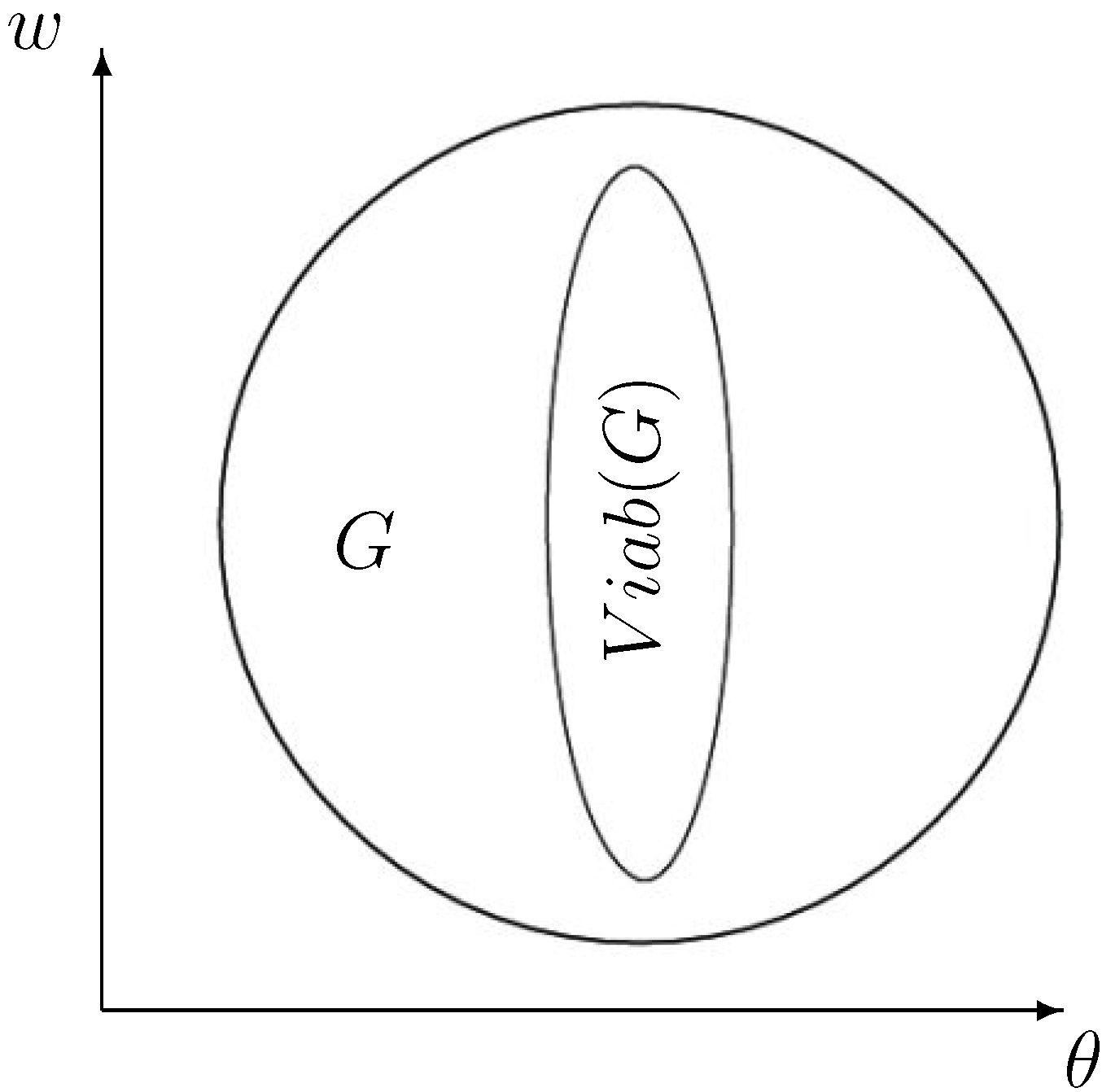
which is the stopping criterion. The runtime on a laptop with six threads is approximately 1 min. Figure 1 shows the viability kernel obtained as $Viab\left(G\right)=\{(\theta ,w):{\mathcal{V}}_{\ell }^h(\theta ,w)\le 1\}.$

Figure 1. The viability kernel for the problem Equation (15) with the above described data.

Figure 1. The viability kernel for the problem Equation (15) with the above described data.

6. Conclusions

Our experience shows that the grid methods outlined in this paper are appropriate for solving nonlinear problems of the dimension up to four. The next steps will be aimed towards dimensions five and six, which requires the use of sparse representations of grid functions and the supercomputing systems that are available nowadays. Such results will allow us to consider, e.g., aircraft applications related to essentially nonlinear takeoff and landing problems with complex state constraints.