
On the Duality of Discrete and Periodic Functions


Studies conducted at the Institute of Mathematics, Ludwig Maximilians University Munich, 80333 Munich, Germany
Mathematics 2015, 3(2), 299-318; https://0-doi-org.brum.beds.ac.uk/10.3390/math3020299
Submission received: 8 October 2014
/
Accepted: 22 April 2015
/
Published: 30 April 2015
Abstract
:Although versions of Poisson’s Summation Formula (PSF) have already been studied extensively, there seems to be no theorem that relates discretization to periodization and periodization to discretization in a simple manner. In this study, we show that two complementary formulas, both closely related to the classical Poisson Summation Formula, are needed to form a reciprocal Discretization-Periodization Theorem on generalized functions. We define discretization and periodization on generalized functions and show that the Fourier transform of periodic functions are discrete functions and, vice versa, the Fourier transform of discrete functions are periodic functions.
1. Introduction
Versions of Poisson’s summation formula have already been the subject of many publications and it is clear that it plays a very central role in mathematics, physics and electrical engineering. Many publications describe the interaction of discretization (or sampling) and periodization. In some publications we find a clear statement that the Poisson’s Summation Formula (PSF) is linked to both discretization and periodization [1–3], and in rare cases we find that the PSF actually is a discretization-periodization theorem [4]. Despite the circumstance that PSF versions are commonly understood as discretization - periodization relationships, it appears to be difficult to find a simple statement on the special interrelation between discretization and periodization. In this paper, we show that two complementary formulas, very closely related to Poisson’s classical summation formula, are needed to form a complete, i.e., reciprocal, discretization-periodization theorem in the tempered distribution sense.
Most publications about discretization and periodization relationships are so far application driven. A comprehensive derivation of interactions between sampling (discretization) and periodization has already been performed for Gabor systems. Orr and Janssen initially covered the transition from continuous settings to discrete settings [5,6] and later Kaiblinger [7] covered the transition from discrete settings to continuous settings. Finally, Søndergaard summarized and complemented these results in [8] and, amongst other things, wrote a Poisson Summation Formula without sums but with sampling and periodization operators instead ([4], Theorem A.1), very similar to the derivation in this paper but in S0(ℝ), Feichtinger’s algebra [9].
Another comprehensive treatment of interactions between discretization and periodization is given in Ozaktas [10], whereby discreteness and periodicity are characterized as Fourier duals such as translation and modulation. Amongst others, the notion of discrete functions is clarified as being Fourier duals of periodic functions. Other publications establish a connection between sampling and periodization, on the one hand, and Shannon’s Sampling Theorem on the other [11] without compelling necessity to mention Poisson’s summation formula in this context. There are even excellent signal processing textbooks that can manage without Poisson’s summation formula but not without describing its impacts, e.g., [12]. Poisson’s summation formula also plays an important role in wavelet theory [13–15], although only in proofs, because it provides transitions from continuous to discrete settings.
Lastly, Benedetto and Zimmermann investigated the validity of Poisson’s summation formula in several classical spaces in analysis including the space of tempered distributions [3,16]. They define sampling and periodization operators and, amongst others, characterize uniform sampling as the Fourier transform of periodization.
The Poisson Summation Formula is also honored as being the link between the classical Fourier transform and Fourier series in Girgensohn [17], Hunter and Nachtergaele [18] and Strichartz [19]. Indeed, we will see that this link is discretization, formally correct only in the sense of generalized functions, called distributions. Hence, in order to formally treat discrete functions correctly, we will need the theory of distributions, basically developed by Laurent Schwartz in [20,21], with contributions by Temple [22] and Lighthill [2], Gelfand and Schilow [23,24] and Zemanian [25]. For our purposes, it is especially convenient to show everything within the space of tempered distributions
, because the Fourier transform of a tempered distribution is again a tempered distribution [21,26]. Note that the Fourier transform definition can even be more generalized to spaces larger than
, see [27] for example, but extending these results accordingly is beyond the scope of this paper.
Conversely, results presented in this paper may also hold in less general settings. For engineering purposes, it often suffices to apply the definitions of both sampling and periodization and use their symbols, but neglect their tempered distribution nature, in order to simplify the already established formulas found in textbooks. A first impression of this technique is given in Section 5 that uses almost no generalized functions theory.
Section 2 will first familiarize the reader with the notations used throughout this article. Section 3 explains the proof method; readers familiar with distribution theory may skip this section. In Section 4 we define discretization and periodization as operations on suitable subspaces of tempered distributions and in Section 5 we hope to motivate the reader to apply them to already known results in textbooks. Section 6 provides calculation rules for both discretization and periodization, such that the proof of our theorem in Section 7 reduces to two lines. Finally, we summarize our results in Section 8 and provide an outlook in Section 9.
2. Notation
We mainly follow established notations as in Schwartz [21], including his Fourier transform definition Equation (1), Benedetto [3], Strichartz [26] and Walter [27], and we substantially follow Woodward [1] and Bracewell [28]. One of the primary goals of this paper is to extend Bracewell’s idea of establishing symbolic calculation rules in signal processing for educational purposes. His textbook Fourier Transform and its Applications is a highly recognized standard work in electrical engineering literature. By replacing Bracewell’s Shah symbol III by two Shah-like symbols
and
we achieve three things: (1) we are able to express the interrelation between discretization and periodization, (2) we are able to express the duality of both symbols and (3) we overcome difficulties that arise when conventional dissimilar symbols are used.
The application of a distribution
to some test function
is denoted as ⟨f, φ⟩ and, in particular, if f is a locally integrable function such that the following integral exists, we define it by
For singular distributions, e.g.,
, it is required to write down their definition explicitly, i.e., ⟨δ, φ⟩ := φ(0). The Fourier Transform for integrable functions φ ∈ L1(ℝn) is defined by
where
and t · σ is the usual scalar product in ℝn. For generalized functions
we define its Fourier transform by
i.e., is “rolled off” to test functions φ, a standard technique for definitions in distribution theory. Defining the Fourier transform in that way implies that δ = 1 and 1 = δ, see for example [21]. Also note that −1 f = f and −1 f = f for any
, see [21,26], and
where
for test functions
. Furthermore, we define Fourier Series S for integrable periodic functions f ∈ L1(ℝn) by
The translation operator τ for some function
and some constant a ∈ ℝn is defined by (τaf)(t) := f(t − a). For generalized functions it is defined by
Additionally, we abbreviate τaδ:= δa for translated Dirac impulses δ. Often in the literature we find a Dirac impulse train, also Dirac comb as
Instead of δk, we often use δkT where
. By kT we mean component-wise multiplication with k ∈ ℤn. Note that
, see [2,26,29] for example.
As mentioned already, the Fourier transform of a tempered distribution is again a tempered distribution. So, for convenience, we stay in
. Additionally, we sometimes need to restrict ourselves to several subspaces of
and would like to remind the reader that the following continuous embeddings of distribution spaces
have been investigated in [21]. We will need the space of test functions
, its dual space ′, the space of infinitely differentiable functions with compact support
and the space of bounded test functions and its dual space
, we need the Schwartz space
of rapidly decreasing, infinitely differentiable functions and its dual space, the space of tempered distributions
and exploit that is an automorphism of
, i.e.,
and that this implies that is an automorphism of
, i.e.,
.
Additionally, we require the space of slowly increasing test functions
and the space of rapidly decreasing distributions to be the image of
in
with respect to , i.e.,
and
. Recall that
and
are the spaces of multiplication operators in
and convolution operators in
, respectively [21]. Finally, all those spaces X(ℝn) we abbreviate to X, for functions
depending on t ∈ ℝn we write φ instead of φ(t). For test functions in
we use α, β, for test functions in
we use φ, ψ and for generalized functions in
or
we use f, g.
3. Idea
In signal processing it is well-known that sampling a function means periodizing its spectrum. And, vice versa, periodizing a function means sampling its spectrum. Our goal is now, first, to formulate this in the simplest way and, secondly, to prove it the widest possible way. We are especially interested under which conditions these statements hold in the widest sense.
Denoting a generalized function as f and its spectrum as f, we additionally require a symbol for discretization, say
, and one for periodization, say
. We will then write a sampled function as
and a periodized function as
. This notation is deliberately chosen such that it reminds us of linear algebra notations like y = Ax. Having a symbol for discretization, we are now able to express the relationship between Fourier series s and the Fourier transform as
, i.e., first applying discretization and then to f corresponds to what we know as the Fourier series of f, shortly
where ◦ is concatenation. Now, coming back to the first two sentences in this section, our goal is to prove that
and
in the generalized functions sense if f satisfies suitable properties. But what do these properties look like, why do we need distribution theory and does this really have applications?
Properties. We will see that f must be an element in
to fulfill the first equation, and an element in
to fulfill the second.
3.1. Distribution Theory
Indeed, the only way to prove these equations is using the theory of generalized functions (distribution theory) because sampling some function φ(t), often explained via definition
is mathematically wrong. Either this integral would be zero according to the definition of δ or it contradicts the Lebesgue integral. Distribution theory has been developed to overcome this problem. Instead of the integral expression, we now write
to apply δ to a function φ. The novelty is that arbitrarily defined “functions” f can now be applied to other functions φ without contradicting the Lebesgue integral. Hence, ⟨·, ·⟩ can be considered as a “generalized integral” but, equivalently, we must take care that ⟨f, φ⟩ < ∞ holds for all “functions” f operating on functions φ. This is secured by using spaces X of φ having certain properties and spaces X′ of f with complementary properties. So, for example, if f is slowly growing then φ must be rapidly decreasing. Vice versa, if f is rapidly decreasing then φ is allowed to be slowly growing. Coming back to our equations, we must show that if f ∈ X′ then the above equations, e.g.,
, must hold in the sense that
for every test function φ ∈ X. Also, note that spaces of test functions are continuously embedded in spaces of generalized functions X ⊂ X′, such that test functions themselves are generalized functions. Moreover, in distribution theory every test function φ is required being infinitely differentiable
such that derivatives of generalized functions can always be found no matter whether their derivatives do exist in the conventional sense or not. Distribution theory is therefore also regarded as the completion of Fourier analysis [2] or of differential calculus [26].
3.2. Applications
As usually done in distribution theory, we will claim in the following, e.g., Equations (5), (7), (10), (17), (21) and (23), that all functions involved must be test functions, i.e., they are in
. This is required in order to be able to roll-off the multiplication of functions with generalized functions to the multiplication of functions with test functions in definition ⟨αf, φ⟩ := ⟨f, αφ⟩ such that
is secured for all
. The property of being infinitely differentiable is a pure technical requirement in distribution theory that does not restrict the theorem we prove for two reasons: (1) In distribution theory, every locally integrable function (considered as generalized function) is already infinitely differentiable and (2) distribution theory is connected to its applications via several approximation theorems (see e.g., [27,30]). For example, every continuous function but also every generalized function can be approximated by test functions, i.e., functions in the classical sense being infinitely differentiable. We therefore always operate (as usual) on either spaces of generalized functions or spaces of test functions.
3.3. Generality
The theorem we prove corresponds to the Fourier transform in
, the widest possible comprehension of the Fourier transform as automorphism (according to Laurent Schwartz’ distribution theory [20,21]) and is, hence, most general in this sense. It comprises, moreover, several classical definitions of the Fourier transform. We note, for example, that there is no need to have a special Fourier transform P designed for periodic functions. Also constants, in particular also being periodic functions, can be Fourier transformed without difficulties. Finally, all results presented in this paper can be used in pure symbolic calculations once they have been proven (in
). Our theorem shows that discretization and periodization are intertwined by the Fourier transform, symbolically
and
where · is an operator argument placeholder.
4. Definitions
We often find the Shah symbol III in the literature (Bracewell [28], Feichtinger [31] and Lecture Notes, e.g., [32]) as an abbreviation for the Dirac impulse train Equation (4). It is convenient to only have one symbol because the Dirac impulse train can be used to both discretize and periodize functions: Multiplication with it yields discrete functions, convolution with it yields periodic functions [28]. Furthermore, having only one symbol avoids introducing a theory of operations on functions which is especially of advantage for reasons of brevity in engineering books. However, any interaction between discretization and periodization cannot be expressed via one symbol.
4.1. Discretization
A major difficulty in
is that the product of two tempered distributions is generally not defined. We will therefore use Laurent Schwartz’ [21] space of multiplication operators
in the following definition.
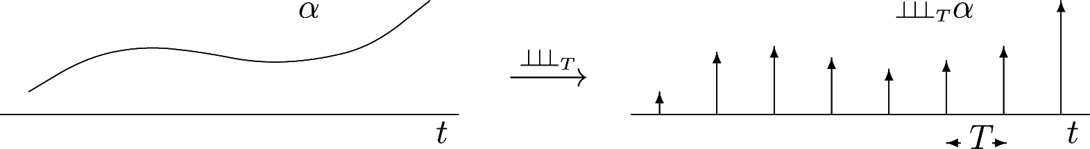
Definition 1 (Discretization). For slowly increasing functions and increments we claim that the tempered distribution defined by
converges in (Figure 1). The operation is called uniform discretization (or sampling) with increments T. We call the discrete (sampled) function of α discretized (sampled) with increments T. Discretization (sampling) is a linear continuous operator,
. We abbreviate, if α is discretized (sampled) with increments Tν = 1 in all dimensions 1 ⩽ ν ⩽ n and identify.
Discretization will be well-defined in this sense and it is clear that these series indeed converge in
, see [26] for example. This definition corresponds in fact to the multiplication of function α with a Dirac comb
. It is today already a common engineering practice to model the sampling process by the multiplication with the Dirac comb [33]. However, an operator approach is much more advantageous as we will see later. It can already be found as combT (α) in [1], later re-published in [34].
4.2. Periodization
Analogous to discretization where the space of multiplication operators
in
is required, we will now need the space of convolution operators
in
, again, introduced by Laurent Schwartz in [21].
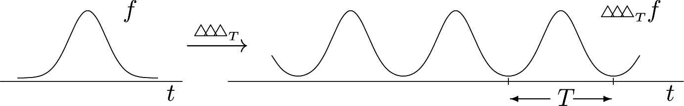
Definition 2 (Periodization). For rapidly decreasing tempered distributions and increments we claim that the tempered distribution defined by
converges in (Figure 2). The operation is called periodization (replicating) or periodic continuation of f with periods T. Periodization (replicating) is a linear continuous operator,
. We abbreviate if f is periodically continued (replicated) with periods Tν = 1 in all dimensions 1 ⩽ ν ⩽ n and identify.
Again, it is clear that periodization is well-defined in this sense and that these series do converge in
. In some textbooks, this operator can be found as repT f [1,34,35], as fper [15], as
[16], as Pf [26], as
[36] as Tf [37] or as fT [38]. However,
is similar to
and can, hence, be used for symbolic calculations as we will see later. We will in particular see that, by using
and
, especially Poisson Summation Formulas reduce to something that is much easier to understand.
5. Motivation
The interaction of discretization and periodization is ubiquitous in many calculations that we find in today’s textbooks. In order to reveal these relations, in this section we use Equations (5) and (6), for the sake of simplicity, neglect considerations in the tempered distribution sense. We give three examples: first, we show that Fourier Series result from Fourier transforming discretized functions. Secondly, we develop periodized functions into Fourier series seeing that it is related to discretization. And, thirdly, we apply the definitions of Section 4 to known versions of Poisson’s summation formula found in the literature.
5.1. Fourier Series and Fourier Transform
Using our definition of discretization we verify that Fourier series actually correspond to a concatenation of discretization followed by Fourier transformation. Hence, having and
, the definition of S as given in Equation (3) is obsolete; we may now write
instead of introducing Equation (3).
Lemma 1 (Fourier Series vs Fourier Transform). Let, then
Proof. We may apply
to
and, accordingly,
converges in
such that
. Due to the convergence of
in
we may calculate term by term. Symbolically, we obtain
with equalities in the tempered distributions sense. □
A consequence is the following equality in the operations sense
where ○ is the concatenation of operations in
. We will later come back to this result in Equation (25).
5.2. Fourier Series of Periodized Functions
For further motivation we show that a Discretization-Periodization Theorem for Schwartz functions
can already be derived from the above definitions: We construct the Fourier series of a periodically continued function
and see that it is indeed related to discretization. Note that every periodic function f can be written as
for some function ϕ. Because
it follows that
is a tempered distribution. As every periodic function can be developed into a sum of ek(t) = e2πi t·k, k ∈ ℤn, we will now do this for
. Starting from
we finally arrive at (see [27,39,40] for example)
Inserting now the definition of discretization yields this important relationship, a formula being closely related to Poisson’s summation formula, between periodization and discretization
so far for Schwartz functions
. We note that
such that
is meaningful as well because
requires functions in
according to Definition 1.
Indeed, Equation (10) can be more generalized and an inversion formula can be found. It will, moreover, be surprising to learn at this point that both operators in Equations (5) and (6) have already been defined in Woodward’s 1953 textbook [1] leading to Equations (28) and (29), meant on functions in
. In Section 7, we will extend these results to generalized functions
and
(see also Appendix B).
5.3. Versions of Poisson Summation Formulas
In general, each Poisson Summation Formula is only one of two possible statements: It either turns discretization into periodization resulting in Equations (23) and (28) or it turns periodization into discretization resulting in Equations (24) and (29) via the Fourier transform. And special cases lead to Equations (16) and (27). This can be seen by applying Equations (5) and (6) to PSF versions found in the literature. In the following we distinguish a general version, a classical version, a symmetrical version and, finally, a special version.
For simplicity, let
and T ∈ ℝ+ (one-dimensional case) for now. Recall that PSF are valid on
, see e.g., [3,9]. In Section 7, we will extend these results to generalized functions
and
(see also Appendix B). We note that Equation (11) corresponds to Equations (24) and (29) in Section 7.
A general version of Poisson’s summation formula can be found for example as
in Benedetto and Zimmermann [3] but also in [16,37,38,41–43]. Inserting Equations (5) and (6) and using Equation (9), this formula yields (29). A variation of (11) emerges if T = 1, e.g., in Gröchenig [39].
Now, let t ≡ 0, then Equation (11) reduces to the classical version of Poisson’s summation formula
found in [1–3,43–45] for example.
Now, let T ≡ 1, then Equation (12) reduces to the symmetrical version of Poisson’s summation formula
where
, e.g., found in Feichtinger and Strohmer [9], also in [37,46–48]. We note that the latter two Equations (12) and (13), especially the last one, look most elegant and one might guess that there would be some loss of information from top to bottom. But surprisingly, the deduction could also be done from bottom to top, first via argument substitution x ↦ xT, i.e., using Fourier transform rule (φ(xT)) = (1/T) (φ)(x/T) and then using argument substitution x ↦ t + x, i.e., using Fourier transform rule (φ(t + x)) = (φ)(x) e2πit·x. Hence, Equations (11), (12) and (13) can be transferred into one another for.
Now, let us assume that instead of
, we indeed have some suitable
, let f ≡ δ, then Equation (11) is valid in
(known result) and reduces to the special version of Poisson’s summation formula
also found very often in the literature, for example in [16,26,39,49] stating that the Fourier transform of a Dirac comb is a Dirac comb. Thus, Equation (11) with f ≡ δ yields (27). Additionally having T = 1 yields (16), found for example in [3,16,50,51]. Note that in Equation (14) we already use identity
. Such rules will be treated in the next section.
Finally, by looking at the from bottom-to-top derivation above, we note that there is a certain degree of freedom on what side to move the Fourier transform. This allows us, in contrast to what is already done, to periodize f instead of f, resulting in the other two Equations (23) and (28) we will prove in Section 7. These formulas are, in contrast to Equations (24) and (29), very difficult to find in the literature. However, [52] is one of the rare sources where beside the classical Poisson Summation Equation (37.1) in [52] another dual formula Equation (37.2) in [52] can be found instead of only one; Equation (37.2) in [52] corresponds to Equations (23) and (28) and Equation (37.1) in [52] corresponds to Equations (24) and (29).
6. Calculation Rules
In order to present a concise proof of Theorem 1, we need to compile few important operator properties. We note that the Fourier transform of a Dirac comb within
is commonly known (e.g., [16,39]) whereas the (asymmetric) duality of multiplication and convolution within
is a more generalized case of commonly known (symmetric) versions (e.g., in
), it can be found in [21].
Dirac Comb Identity. The first, maybe surprising observation by looking at the two definitions above is that both operations generate a Dirac impulse train by either sampling the function that is constantly 1 or by periodically repeating δ, symbolically
Moreover, 1 and δ are unitary elements with respect to multiplication and convolution in
, respectively. They are also a Fourier pair, more precisely 1 = δ and δ = 1. Also note that the Shah symbol III in Equation (4) is called the sampling or replicating symbol in [28] because it can be used for either sampling (discretizing) or replicating (periodizing) a function. However, instead of III we now have either
or, alternatively,
which allows us to switch from discretization to periodization or from periodization to discretization (needed in proof of Theorem 1).
Dirac Comb Fourier Transform. We also need that
and, accordingly,
Omitting Brackets. A very convenient property of both operators is that brackets can be omitted. For reasons of brevity, we move this proof to Appendix A.
Lemma 2. Let and. Then
In particular, with
, additionally let us identify
and
, with Equations (17) and (18) we obtain relationships published in Bracewell [28]
It means that discretization is realized via multiplication and periodization is realized via convolution with III. Note that replacing III by operations
,
is the central proposal in this paper.
Multiplication and Convolution. Recall that multiplication or convolution products do not necessarily exist in
. We must rather restrict our operator arguments to suitable subspaces of
(see operator definitions), i.e., to
and
respectively.
Lemma 3 (Multiplication and Convolution). Let
and
. Then
A detailed treatment of multiplication and convolution in
including a proof of this lemma is given in [21], Théorème XV, p. 124. Notice that
can rarely be found in the literature ([30,53–56]) while
is better known. A description of interactions of
with
, aside from [21], is even more seldom in the literature, e.g., [57,58] describing the Fourier transform as an algebra isomorphism
.
7. The Discretization-Periodization Theorem
For the sake of simplicity, we first consider only increments of Tν = 1 in all dimensions 1 ⩽ ν ⩽ n and then generalize these results in a corollary below.
7.1. Unitary Increments
Everything is prepared now to present a discretization - periodization theorem in
. It consists of two formulas very closely related to Poisson’s Summation Formula starting from discretization and from periodization, respectively. Compared to classical versions of Poisson’s summation formula we simply hide one sum in
and the other in
, such that these formulas become better understandable.
Theorem 1 (Discretization vs. Periodization, unitary case). Let and. Then
Note that, in contrast to
and
, both formulas hold for Schwartz functions
understood as rapidly decreasing tempered distributions because
on the one hand, and
on the other. Hence, it proves Equation (10) in particular (see Appendix B).
Furthermore, recall that
and
are the Fourier series S of α according to Equation (7). It is, in other words, the Fourier transform of discrete functions S. And the second equation corresponds to the Fourier transform of periodic functions P (Figure 3). See one-page summaries: Figure 3.31 in [12] or Prolog II in [16], for example, embracing all four different Fourier transforms and Fourier series including their (either integral or discrete) inversion formulas.
Proof. Formally, according to the calculation rules shown above the following equalities hold
in
. We start using f = δ ∗ f because
is the unitary element with respect to convolution in
. Then we apply Equations (18), (22), (16), (15) and (17), in this order. Finally, let
, we use α = 1·α because
is the unitary element with respect to multiplication in
to show the second formula in an analogous manner. □
To demonstrate the usefulness of the theorem, we use Equations (23), (24) and (15) to prove Equation (16) by
and identifying
and
we obtain
and
.
Finally, we use the theorem to conclude that Equation (8) is complemented having
in the operations sense :
. Hence, Fourier series S either correspond to discretization followed by the Fourier transform or, equivalently, they correspond to the Fourier transform followed by periodization. Accordingly, for the second Poisson Summation Formula (24) we obtain
in the operations sense :
.
7.2. Arbitrary Increments
In our Equations (1), (3) and (4) as well as in Equations (16), (23) and (24) we used periodic functions with periods of Tν = 1 in all dimensions 1 ⩽ ν ⩽ n, which is convenient but not the general case. The following lemma helps to generalize our results to arbitrary periods and increments.
Lemma 4 (Reciprocity). The Fourier transform of a stretched/compressed Dirac impulse train is a compressed/stretched Dirac impulse train. Formally, let then
with
and Tp :T1T2…Tn ∈ ℝ+
A proof of this lemma is straight forward from what is known in the literature (see for example [16,32,40,49]). We will omit it here for the sake of conciseness. Let us now see the theorem in the arbitrary increments case.
Corollary 1 (Discretization vs. Periodization, general case). Let and and let then
where Tp := T1T2…Tn ∈ ℝ+.
This is instantly verified replacing Equation (16) by Equation (27) in the above proof.
8. Conclusions
We have seen that, in the generalized functions sense, there is a (Fourier transform) duality between discrete and periodic functions. The theorem states that the generalized function being discretized must not grow faster than polynomials and the generalized function being periodized must rapidly decay to zero in order to obtain convergence on both sides of the equations in the generalized functions sense. Furthermore, it is shown that both formulas in this theorem are closely related to the classical Poisson Summation Formula. This means that these conditions will have impact on the validity of Poisson Summation Formula versions. We have, furthermore, seen that one formula in this theorem corresponds to Fourier series and the other formula corresponds to the Fourier transform of periodic functions. Finally, by choosing two similar symbols for discretization and periodization, we showed that an easy-to-use symbolic calculation scheme is obtained.
9. Outlook
The theorem above is indisputably connected to the classical sampling theorem, see, e.g., Woodward [1] or Benedetto and Zimmermann [3]. An all-embracing theory including the Sampling Theorem will, however, require to have two more operations, one reversing discretization and one reversing periodization, i.e., interpolation of discrete functions and restriction of a periodic function to one period. Surprisingly, S′ has been suitable to model discretization and periodization but will not be suitable to model their inverses. Further studies are required.
MSC classifications: 46F10, 46F12
Conflicts of Interest
The author declares no conflicts of interest.
Appendix
A. Proof
Proof of Lemma 2. Discretization,
. We know that
and with
it follows that
such that it can be applied to test functions
. Due to the convergence of
in S′ and the continuity of multiplication :
we may calculate term by term
for all test functions
, i.e.,
. Finally, the roles of α and β can be exchanged due to commutativity
. □
Proof of Lemma 2. Periodization,
. We know that
and with
it follows that
such that it can be applied to test functions
. Due to the convergence of
in
and the continuity of convolution
we may calculate term by term, we use Equations (A3), (A4), (A5), (A3), (A4), in this order, obtaining
for all test functions
, i.e.,
in
. Finally, the roles of f and g can be exchanged due to commutativity f g = g f in
. □
The following definitions and calculation rules are needed for the above proof.
Definition A1. Let and. Then
defines a convolution inwhere.
Lemma A1. Letand. Then where
Proof. We may write
according to Equation (A1),
, Equation (2), (tφ) = e2i t·σ φ, in this order. Because
, we know that Ff is a regular function, hence
The last expression is a function in
because with
and
it follows that
. Finally,
because is an automorphism in
. □
Definition A2. Let and. According to Equation (A2) it follows that such that
defines a convolution in where and.
Lemma A2. Letand. Then
Proof. Let us initially operate on finite sums over k ∈ ℤn with |k| ⩽ N ∈ ℕ where |k| := max1⩽ν ⩽n |kν| is the maximum norm, and let
It then follows that φN ∈ , the space of bounded test functions [21] and
. With finite sums we start operating
on φN ∈ obtaining
where
operates on
. Finally, using the continuity in generalized function spaces
In this last expression we apply a generalized function
to some test function
. We must justify that this makes sense as
and are no dual spaces. But
is continuously embedded in
which is the dual space of such that the convergence of
is secured for all
and
. And the following expressions converge due to the completeness of
in the sense of convergence in
. □
Lemma A3. Let and, then
Proof. With Equation (A2) we know that
and because
we may apply
to f φ and obtain
using Equations (6) and (A1), exchanges in the sequence of translations and again Equation (A1), in this order. □
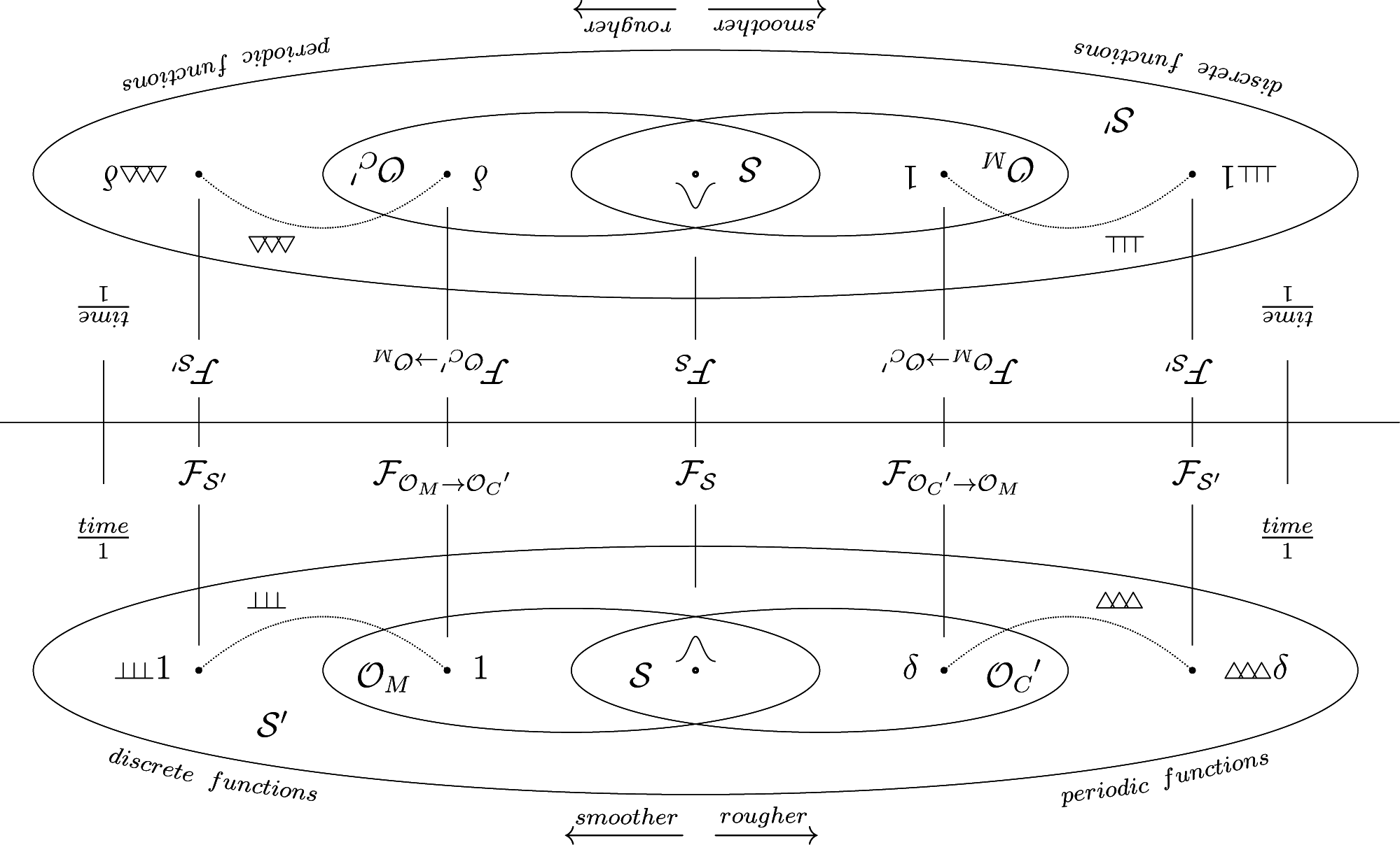
B. Summary
Let us now have a look at the beauty of “sortedness” of functions in S′ (Figure 4). It is this “sortedness” that led us from constant function 1 via the Gaussian function
up to the discovery of δ.
It is interesting to observe that there is a triplet of embedded automorphisms
involved in this scheme where
.
Also note that discrete functions are being injected on the smooth side of S′ (left) whereas periodic functions are being injected on the rough side of
(right). But both are actually located on the same side of
(opposite of
) because left hand side and right hand side are being identical, recall that
. So,
reminds us of a torus.
Acknowledgments
These studies have essentially been conducted at the Ludwig Maximilians University Munich, Institute of Mathematics in 1996. The author is particularly grateful to Professor Otto Forster who made this study possible, especially for directing the authors interests towards Laurent Schwartz’ distribution theory. The author is also very grateful to Professor Hans G. Feichtinger, University of Vienna, for many valuable hints and fruitful discussions and, finally, to the anonymous reviewers who significantly helped improving this manuscript.
References
- Woodward, P.M. Probability and Information Theorywith Applications to Radar; Pergamon Press Ltd: Oxford, UK, 1953. [Google Scholar]
- Lighthill, M.J. An Introduction to Fourier Analysis and Generalised Functions; Cambridge University Press: Cambridge, NY, USA, 1958. [Google Scholar]
- Benedetto, J.J.; Zimmermann, G. Sampling Multipliers and the Poisson Summation Formula. J. Fourier Anal. Appl. 1997, 3, 505–523. [Google Scholar]
- Søndergaard, P.L. Gabor Frames by Sampling and Periodization. Adv. Comput. Math. 2007, 27, 355–373. [Google Scholar]
- Orr, R.S. Derivation of the Finite Discrete Gabor Transform by Periodization and Sampling. Signal Process 1993, 34, 85–97. [Google Scholar]
- Janssen, A. From Continuous to Discrete Weyl-Heisenberg Frames through Sampling. J. Fourier Anal. Appl. 1997, 3, 583–596. [Google Scholar]
- Kaiblinger, N. Approximation of the Fourier Transform and the Dual Gabor Window. J. Fourier Anal. Appl. 2005, 11, 25–42. [Google Scholar]
- Søndergaard, P.L. Finite Discrete Gabor Analysis. Ph.D. Thesis, Institute of Mathematics, Technical University of Denmark, Copenhagen, Denmark, 2007. [Google Scholar]
- Feichtinger, H.G.; Strohmer, T. Gabor Analysis and Algorithms: Theory and Applications; Birkhäuser: Basel, Switzerland, 1998. [Google Scholar]
- Ozaktas, H.M.; Sumbul, U. Interpolating between Periodicity and Discreteness through the Fractional Fourier Transform. IEEE Trans. Signal Process. 2006, 54, 4233–4243. [Google Scholar]
- Strohmer, T.; Tanner, J. Implementations of Shannon’s Sampling Theorem, a Time-Frequency Approach. Sampl. Theory Signal Image Process 2005, 4, 1–17. [Google Scholar]
- Proakis, J.G.; Manolakis, D.G. Digital Signal Processing: Principles, Algorithms and Applications, 2nd ed; Macmillan Publishers: Greenwich, CT, USA, 1992. [Google Scholar]
- Heil, C.E.; Walnut, D.F. Continuous and Discrete Wavelet Transforms. SIAM Rev. 1989, 31, 628–666. [Google Scholar]
- Daubechies, I. The Wavelet Transform, Time-Frequency Localization and Signal Analysis. IEEE Trans. Inf. Theory 1990, 36, 961–1005. [Google Scholar]
- Daubechies, I. Ten Lectures on Wavelets; Society for Industrial and Applied Mathematics (SIAM): Philadelphia, PA, USA, 1992. [Google Scholar]
- Benedetto, J.J. Harmonic Analysis Applications; CRC Press: Boca Raton, FL, USA, 1996. [Google Scholar]
- Girgensohn, R. Poisson Summation Formulas and Inversion Theorems for an Infinite Continuous Legendre Transform. J. Fourier Anal. Appl. 2005, 11, 151–173. [Google Scholar]
- Hunter, J.K.; Nachtergaele, B. Applied Analysis; World Scientific Publishing Company: Singapore, 2001. [Google Scholar]
- Strichartz, R.S. Mock Fourier Series and Transforms Associated with Certain Cantor Measures. J. Anal. Math. 2000, 81, 209–238. [Google Scholar]
- Schwartz, L. Théorie des Distributions Tome I; Hermann Paris: Paris, France, 1950. [Google Scholar]
- Schwartz, L. Théorie des Distributions Tome II; Hermann Paris: Paris, France, 1959. [Google Scholar]
- Temple, G. The Theory of Generalized Functions. Proc. R. Soc. Lond. Ser. A Math. Phys. Sci. 1955, 228, 175–190. [Google Scholar]
- Gelfand, I.; Schilow, G. Verallgemeinerte Funktionen (Distributionen), Teil I; VEB Deutscher Verlag der Wissenschaften Berlin: Berlin, Germany, 1969. [Google Scholar]
- Gelfand, I.; Schilow, G. Verallgemeinerte Funktionen (Distributionen), Teil II, Zweite Auflage; VEB Deutscher Verlag der Wissenschaften Berlin: Berlin, Germany, 1969. [Google Scholar]
- Zemanian, A. Distribution Theory And Transform Analysis—An Introduction To Generalized Functions, With Applications; McGraw-Hill Inc: New York, NY, USA, 1965. [Google Scholar]
- Strichartz, R.S. A Guide to Distribution TheorieFourier Transforms, 1st Ed ed; CRC Press: Boca Raton, FL, USA, 1994. [Google Scholar]
- Walter, W. Einführung in die Theorie der Distributionen; BI-Wissenschaftsverlag, Bibliographisches Institut & FA Brockhaus: Mannheim, Germany, 1994. [Google Scholar]
- Bracewell, R.N. Fourier Transform its Applications; McGraw-Hill Book Company: New York, NY, USA, 1965. [Google Scholar]
- Nashed, M.Z.; Walter, G.G. General Sampling Theorems for Functions in Reproducing Kernel Hilbert Spaces. Math. Control Signals Syst. 1991, 4, 363–390. [Google Scholar]
- Grubb, G. Distributions and Operators; Springer: Berlin, Germany, 2008. [Google Scholar]
- Feichtinger, H.G. Atomic Characterizations of Modulation Spaces through Gabor-Type Representations. Rocky Mt. J. Math 1989, 19, 113–125. [Google Scholar]
- Osgood, B. The Fourier Transform and its Applications; Lecture Notes for EE 261; Electrical Engineering Department, Stanford University: Stanford, CA, USA, 2005. [Google Scholar]
- Unser, M. Sampling-50 Years after Shannon. IEEE Proc. 2000, 88, 569–587. [Google Scholar]
- Brandwood, D. Fourier Transforms in Radar and Signal Processing; Artech House: Norwood, MA, USA, 2003. [Google Scholar]
- Cariolaro, G. Unified Signal Theory; Springer: Berlin, Germany, 2011.
- Jerri, A. Integral and Discrete Transforms with Applications and Error Analysis; Marcel Dekker Inc: New York, NY, USA, 1992. [Google Scholar]
- Auslander, L.; Meyer, Y. A Generalized Poisson Summation Formula. Appl. Comput. Harmon. Anal. 1996, 3, 372–376. [Google Scholar]
- Brigola, R. Fourieranalysis Distributionenund Anwendungen; Vieweg Verlag: Wiesbaden, Germany, 1997. [Google Scholar]
- Gröchenig, K. Foundations of Time-Frequency Analysis; Birkhäuser: Basel, Switzerland, 2001. [Google Scholar]
- Quegan, S. Signal Processing; Lecture Notes; University of Sheffield: Sheffield, UK, 1993.
- Gröchenig, K. An Uncertainty Principle related to the Poisson Summation Formula. Stud. Math. 1996, 121, 87–104. [Google Scholar]
- Papoulis, A.; Pillai, S.U. Probability Random Variables, and Stochastic Processes; Tata McGraw-Hill Education: Noida, India, 1996. [Google Scholar]
- Li, B.Z.; Tao, R.; Xu, T.Z.; Wang, Y. The Poisson Sum Formulae Associated with the Fractional Fourier Transform. Signal Process. 2009, 89, 851–856. [Google Scholar]
- Rahman, M. Applications of Fourier Transforms to Generalized Functions; Wessex Institute of Technology (WIT) Press: Ashurst Lodge UK, 2011. [Google Scholar]
- Jones, D. The Theory of Generalized Functions; Cambridge University Press: Cambridge, UK, 1982. [Google Scholar]
- Kahane, J.P.; Lemarié-Rieusset, P.G. Remarques sur la formule sommatoire de Poisson. Stud. Math. 1994, 109, 303–316. [Google Scholar]
- Balazard,, M.; France,, M.M.; Sebbar,, A. Variations on a Theme of Hardy’s. Ramanujan J. 2005, 9, 203–213. [Google Scholar]
- Lev, N.; Olevskii, A. Quasicrystals and Poisson’s Summation Formula. Invent. Math. 2013. [Google Scholar] [CrossRef]
- Mallat, S. A Wavelet Tour of Signal Processing; Academic Press: Waltham, MA, USA, 1999. [Google Scholar]
- Feichtinger, H.G. Elements of Postmodern Harmonic Analysis. In Operator-Related Function Theory and Time-Frequency Analysis; Springer: Berlin, Germany, 2015; pp. 77–105. [Google Scholar]
- Lev, N.; Olevskii, A. Measures with Uniformly Discrete Support and Spectrum. Compt. Rendus Math. 2013, 351, 599–603. [Google Scholar]
- Gasquet, C.; Witomski, P. Fourier Analysis and Applications: Filtering, Numerical Computation, Wavelets; Springer: Berlin, Germany, 1999. [Google Scholar]
- Edwards, R. On Factor Functions. Pac. J. Math. 1955, 5, 367–378. [Google Scholar]
- Betancor, J.J.; Marrero, I. Multipliers of Hankel Transformable Generalized Functions. Comment. Math. Univ. Carolin 1992, 33, 389–401. [Google Scholar]
- Bonet, J.; Frerick, L.; Jordá, E. The Division Problem for Tempered Distributions of One Variable. J. Funct. Anal. 2012, 262, 2349–2358. [Google Scholar]
- Morel, J.M.; Ladjal, S. Notes sur l’analyse de Fourier et la théorie de Shannon en traitement d’images. J. X-UPS 1998, 1998, 37–100. [Google Scholar]
- Gracia-Bondía, J.M.; Varilly, J.C. Algebras of Distributions Suitable for Phase-Space Quantum Mechanics. I. J. Math. Phys. 1988, 29, 869–879. [Google Scholar]
- Dubois-Violette, M.; Kriegl, A.; Maeda, Y.; Michor, P.W. Smooth*-Algebras. Prog. Theor. Phys. Supp. 2001, 144, 54–78. [Google Scholar]
Figure 1.
Discretization of regular function yielding generalized function ???T.

Figure 2.
Periodization of generalized function f yielding generalized function △△△T f.

Figure 3.
The Discretization-Periodization Theorem.

Figure 4.
The space of tempered distributions and important subspaces.

© 2015 by the authors; licensee MDPI, Basel, Switzerland This article is an open access article distributed under the terms and conditions of the Creative Commons Attribution license (http://creativecommons.org/licenses/by/4.0/).
Share and Cite
MDPI and ACS Style
Fischer, J.V. On the Duality of Discrete and Periodic Functions. Mathematics 2015, 3, 299-318. https://0-doi-org.brum.beds.ac.uk/10.3390/math3020299
AMA Style
Fischer JV. On the Duality of Discrete and Periodic Functions. Mathematics. 2015; 3(2):299-318. https://0-doi-org.brum.beds.ac.uk/10.3390/math3020299
Chicago/Turabian StyleFischer, Jens V. 2015. "On the Duality of Discrete and Periodic Functions" Mathematics 3, no. 2: 299-318. https://0-doi-org.brum.beds.ac.uk/10.3390/math3020299