Numerical Solution of Fractional Differential Equations: A Survey and a Software Tutorial

Abstract

Solving differential equations of fractional (i.e., non-integer) order in an accurate, reliable and efficient way is much more difficult than in the standard integer-order case; moreover, the majority of the computational tools do not provide built-in functions for this kind of problem. In this paper, we review two of the most effective families of numerical methods for fractional-order problems, and we discuss some of the major computational issues such as the efficient treatment of the persistent memory term and the solution of the nonlinear systems involved in implicit methods. We present therefore a set of MATLAB routines specifically devised for solving three families of fractional-order problems: fractional differential equations (FDEs) (also for the non-scalar case), multi-order systems (MOSs) of FDEs and multi-term FDEs (also for the non-scalar case); some examples are provided to illustrate the use of the routines.

1. Introduction

The increasing interest in applications of fractional calculus has motivated the development and the investigation of numerical methods specifically devised to solve fractional differential equations (FDEs). Finding analytical solutions of FDEs is, indeed, even more difficult than solving standard ordinary differential equations (ODEs) and, in the majority of cases, it is only possible to provide a numerical approximation of the solution.

Although several computing environments (such as, for instance, Maple, Mathematica, MATLAB and Python) provide robust and easy-to-use codes for numerically solving ODEs, the solution of FDEs still seems not to have been addressed by almost all computational tools, and usually, researchers have to write codes by themselves for the numerical treatment of FDEs.

When numerically solving FDEs, one faces some non-trivial difficulties, mainly related to the presence of a persistent memory (which makes the computation extremely slow and expensive), to the low-order accuracy of the majority of the methods, to the not always straightforward computation of the coefficients of several schemes, and so on.

Writing reliable codes for FDEs can be therefore a quite difficult task for researchers and users with no particular expertise in computational mathematics, and it would be surely preferable to rely on efficient and already tested routines.

The aim of this paper is to illustrate the basic principles behind some methods for FDEs, thus to provide a short tutorial on the numerical solution of FDEs, and discuss some non-trivial issues related to the effective implementation of methods as, for instance, the treatment of the persistent memory term, the solution of equations involved by implicit methods, and so on; at the same time, we present some MATLAB routines for the solution of a wide range of FDEs.

This paper is organized as follows. In Section 2, we recall some basic definitions concerning fractional-order operators, and we present some of the most useful properties that will be used throughout the paper. Section 3 is devoted to illustrating multi-step methods for FDEs; in particular, we discuss product-integration (PI) rules and Lubich’s fractional linear multi-step methods (FLMMs); we also discuss in detail the main issues and advantages related to the use of implicit methods, and we illustrate a technique based on the fast Fourier transform (FFT) algorithm to efficiently treat the persistent memory term.

In Section 4, we consider two special cases of FDEs: multi-order systems (MOSs) in which each equation has a different fractional-order and multi-term FDEs in which there is more than one fractional derivative in a single equation; in particular, we will see how standard methods studied in the previous section can be adapted to solve these particular problems.

In Section 5, we present some MATLAB routines for solving different families of FDEs and explain their use in detail; finally, Section 6 is devoted to showing the application of the routines to a selection of test problems.

2. Preliminary Material on Fractional Calculus

For the sake of clarity, we review in this section some of the most useful definitions in fractional calculus, and we recall the properties that we will use in the subsequent sections. For a more comprehensive introduction to this subject, the reader is referred to any of the available textbooks [1,2,3,4,5] or review papers [6,7] and, in particular, to the book by Diethelm [8] by which this introductory section is mainly inspired.

As the starting point for introducing fractional-order operators, we consider the Riemann–Liouville (RL) integral; for a function $y\left(t\right)\in L^1\left([t_0,T]\right)$ (as usual, $L^1$ is the set of Lebesgue integrable functions), the RL fractional integral of order $\alpha >0$ and origin at $t_0$ is defined as:

$$J_{t_0}^{\alpha }y\left(t\right)=\frac{1}{\Gamma \left(\alpha \right)}{\int }_{t_0}^t{(t-\tau )}^{\alpha -1}y\left(\tau \right)\mathrm{d}\tau .$$

(1)

It provides a generalization of the standard integral, which, indeed, can be considered a particular case of the RL integral (1) when $\alpha =1$. The left inverse of $J_{t_0}^{\alpha }$ is the RL fractional derivative:

$${\widehat{D}}_{t_0}^{\alpha }y\left(t\right):=D^m{J}_{t_0}^{m-\alpha }y\left(t\right)=\frac{1}{\Gamma (m-\alpha )}\frac{{\mathrm{d}}^m}{\mathrm{d}{t}^m}{\int }_{t_0}^t{(t-\tau )}^{m-\alpha -1}y\left(\tau \right)\mathrm{d}\tau ,$$

(2)

where $m=⌈\alpha ⌉$ is the smallest integer greater or equal to $\alpha$ and $D^m$, $y^{\left(m\right)}$ or ${\mathrm{d}}^m/\mathrm{d}{t}^m$ denotes the standard integer-order derivative.

An alternative definition of the fractional derivative, obtained after interchanging differentiation and integration in Equation (2), is the so-called Caputo derivative, which, for a sufficiently differentiable function, namely for $y\in A^m\left([t_0,T]\right)$ (i.e., $y^{(m-1)}$ absolutely continuous), is given by:

$$D_{t_0}^{\alpha }y\left(t\right):=J_{t_0}^{m-\alpha }{D}^{m}y\left(t\right)=\frac{1}{\Gamma (m-\alpha )}{\int }_{t_0}^t{(t-\tau )}^{m-\alpha -1}{y}^{\left(m\right)}\left(\tau \right)\mathrm{d}\tau .$$

(3)

We observe that also $D_{t_0}^{\alpha }y\left(t\right)$ is a left inverse of the RL integral, namely $D_{t_0}^{\alpha }{J}_{t_0}^{\alpha }y=y$ [8] (Theorem 3.7), but not its right inverse, since [8] (Theorem 3.8):

$$J_{t_0}^{\alpha }{D}_{t_0}^{\alpha }y\left(t\right)=y\left(t\right)-T_{m-1}[y;t_0]\left(t\right),$$

(4)

where $T_{m-1}[y;t_0]\left(t\right)$ is the Taylor polynomial of degree $m-1$ for the function $y\left(t\right)$ centered at $t_0$, that is:

$$T_{m-1}[y;t_0]\left(t\right)=\sum _{k=0}^{m-1}\frac{{(t-t_0)}^k}{k!}{y}^{\left(k\right)}\left(t_0\right).$$

More generally speaking, by combining [1] (Lemma 2.3) and [8] (Theorem 3.8), it is also possible to observe that for any $\beta >\alpha$, it holds:

$$J_{t_0}^{\beta }{D}_{t_0}^{\alpha }y\left(t\right)=J_{t_0}^{\beta }{\widehat{D}}_{t_0}^{\alpha }\left[y\left(t\right)-T_{m-1}[y;t_0]\left(t\right)\right]=J_{t_0}^{\beta -\alpha }\left[y\left(t\right)-T_{m-1}[y;t_0]\left(t\right)\right],$$

(5)

a relationship that will be useful, in a particular way, in Section 4.2 on multi-term FDEs.

The two definitions (2) and (3) are interrelated, and indeed, by deriving both sides of Equation (4) in the RL sense, it is possible to observe that:

$$D_{t_0}^{\alpha }y\left(t\right)={\widehat{D}}_{t_0}^{\alpha }\left[y\left(t\right)-T_{m-1}[y;t_0]\left(t\right)\right]$$

and, consequently:

$${\widehat{D}}_{t_0}^{\alpha }y\left(t\right)=D_{t_0}^{\alpha }y\left(t\right)+\sum _{k=0}^{m-1}\frac{{(t-t_0)}^{k-\alpha }}{\Gamma (k+1-\alpha )}{y}^{\left(k\right)}\left(t_0\right).$$

Observe that in the special case $0<\alpha <1$, the above relationship becomes:

$${\widehat{D}}_{t_0}^{\alpha }y\left(t\right)=D_{t_0}^{\alpha }y\left(t\right)+\frac{{(t-t_0)}^{-\alpha }}{\Gamma (1-\alpha )}y\left(t_0\right)$$

clearly showing how the Caputo derivative is a sort of regularization of the RL derivative at $t_0$. Another feature that justifies the introduction of the Caputo derivative is related to the differentiation of constant function; indeed, since:

$${\widehat{D}}_{t_0}^{\alpha }1=\frac{1}{\Gamma (1-\alpha )}{(t-t_0)}^{-\alpha },D_{t_0}^{\alpha }1=0,$$

in several applications, it is preferable to deal with operators for which the derivative of a constant is zero as in the case of Caputo’s derivative.

One of the most important applications of Caputo’s derivative is however in FDEs. Unlike FDEs with the RL derivative, which are initialized by derivatives of non-integer order, an initial value problem for an FDE (or a system of FDEs) with Caputo’s derivative can be formulated as:

$$\left\{\begin{array}{c}{D}_{t_0}^{\alpha }y\left(t\right)=f(t,y\left(t\right))\hfill \\ y\left(t_0\right)=y_0,y^{\prime }\left(t_0\right)=y_0^{\left(1\right)},\cdots ,y^{(m-1)}\left(t_0\right)=y_0^{(m-1)}\hfill \end{array}\right.$$

(6)

where $f(t,y)$ is assumed to be continuous and $y_0,y_0^{\left(1\right)},\cdots ,y_0^{(m-1)}$ are the assigned values of the derivatives at $t_0$. Clearly, initializing the FDE with assigned values of integer-order derivatives is more useful since they have a more clear physical meaning with respect to fractional-order derivatives.

The application to both sides of Equation (6) of the RL integral $J_{t_0}^{\alpha }$, together with Equation (4), leads to the reformulation of the FDE in terms of the weakly-singular Volterra integral equation (VIE):

$$y\left(t\right)=T_{m-1}[y;t_0]\left(t\right)+\frac{1}{\Gamma \left(\alpha \right)}{\int }_{t_0}^t{(t-\tau )}^{\alpha -1}f(\tau ,y\left(\tau \right))\mathrm{d}\tau .$$

(7)

The integral Formulation (7) is surely useful since it allows exploiting theoretical and numerical results already available for this class of VIEs in order to study and solve FDEs.

We stress the nonlocal nature of FDEs: the presence of a real power in the kernel makes it not possible to split the solution of Equation (7) at any point $t_n$ as the solution at some previous point $t_n-h$ plus the increment term related to the interval $[t_n-h,t_n]$, as is common with ODEs.

Furthermore, as proved by Lubich [9], the solution of the VIE (7) presents an expansion in mixed (i.e., integer and fractional) powers:

$$y\left(t\right)=T_{m-1}\left(t\right)+\sum _{i,j\in \mathbb{N}}{(t-t_0)}^{i+j\alpha }{Y}_{i,j},$$

(8)

thus showing a non-smooth behavior at $t_0$; as is well-known, the absence of smoothness at $t=t_0$ poses some problems for the numerical computation since methods based on polynomial approximations fail to provide accurate results in the presence of some lack of smoothness.

3. Multi-Step Methods for FDEs

Most of the step-by-step methods for the numerical solution of differential equations can be roughly divided into two main families: one-step and multi-step methods.

In one-step methods, just one approximation of the solution at the previous step is used to compute the solution and, hence, they are particularly suited when it is necessary to dynamically change the step-size in order to adapt the integration process to the behavior of the solution. In multi-step methods, it is instead necessary to use more previously evaluated approximations to compute the solution.

Because of the persisting memory of fractional-order operators, multi-step methods are clearly a natural choice for FDEs; anyway, although multi-step methods for FDEs are usually derived from multi-step methods for ODEs, when applied to FDEs, the number of steps involved in the computation is not fixed, but it increases as the integration proceeds forward, and the whole history of the solution is involved in each step’s computation.

Multi-step methods for the FDEs (6) are therefore convolution quadrature formulas, which can be written in the general form:

$$y_n={\phi }_n+\sum _{j=0}^n{c}_{n-j}{f}_j,f_j=f(t_j,y_j),$$

(9)

where ${\phi }_n$ and $c_n$ are known coefficients and $t_n=t_0+nh$ is an assigned grid, with a constant step-size $h>0$ just for simplicity; the way in which the coefficients are derived depends on the specific method. In particular, the following two classes of multi-step methods for FDEs are mainly studied in the literature:

• product-integration (PI) rules,
• fractional linear multi-step methods (FLMMs).

Both families of methods are based on the approximation of the RL integral in the VIE (7) and generalize, on different bases, standard multi-step methods for ODEs. They allow one to write general-purpose methods requiring just the knowledge of the vector field of the differential equation.

We must mention that several other approaches have been however discussed in the literature: see, for instance, the generalized Adams methods [10], extensions of the Runge-Kutta methods [11], generalized exponential integrators [12,13], spectral methods [14,15], spectral collocation methods [16], methods based on matrix functions [17,18,19,20], and so on. In this paper, for brevity, we focus only on PI rules and FLMMs, and we refer the reader to the existing literature for alternative approaches.

3.1. Product-Integration Rules

PI rules were introduced by Young [21] in 1954 to numerically solve second-kind weakly-singular VIEs; they hence apply in a natural way to FDEs due to their formulation in Equation (7).

Given a grid $t_n=t_0+nh$, with constant step-size $h>0$, in PI rules, the solution of the VIE (7) at $t_n$ is first written in a piece-wise way:

$$y\left(t_n\right)=T_{m-1}[y;t_0]\left(t_n\right)+\frac{1}{\Gamma \left(\alpha \right)}\sum _{j=0}^{n-1}{\int }_{t_j}^{t_{j+1}}{(t_n-\tau )}^{\alpha -1}f(\tau ,y\left(\tau \right))\mathrm{d}\tau$$

and $f(\tau ,y(\tau \left)\right)$ is approximated, in each subinterval $[t_j,t_{j+1}]$, by means of some interpolant polynomial; the resulting integrals are hence evaluated in an exact way, thus to lead to $y_n$. According to the way in which the approximation is made, explicit or implicit rules are obtained, and this is perhaps the most straightforward way to generalize Adams multi-step methods commonly employed for integer-order ODEs [22].

For instance, to extend to FDEs the (explicit) forward and (implicit) backward Euler methods, it is sufficient to approximate, in each interval $[t_j,t_{j+1}]$, the integrand $f(\tau ,y(\tau \left)\right)$ by the constant values $f(t_j,y_j)$ and $f(t_{j+1},y_{j+1})$, respectively; the resulting methods are:

$$\mathrm{Expl}.\mathrm{PI}\mathrm{Rectangular}:y_n=T_{m-1}[y;t_0]\left(t_n\right)+h^{\alpha }\sum _{j=0}^{n-1}{b}_{n-j-1}^{\left(\alpha \right)}f(t_j,y_j)$$

(10)

and:

$$\mathrm{Impl}.\mathrm{PI}\mathrm{Rectangular}:y_n=T_{m-1}[y;t_0]\left(t_n\right)+h^{\alpha }\sum _{j=1}^n{b}_{n-j}^{\left(\alpha \right)}f(t_j,y_j)$$

(11)

with $b_n^{\left(\alpha \right)}=({(n+1)}^{\alpha }-n^{\alpha })/\Gamma (\alpha +1)$; the term rectangular comes after the underlying quadrature rules used for the integration. In a similar way, when $f(\tau ,y(\tau \left)\right)$ is approximated by the first order interpolant polynomial:

$$f(\tau ,y\left(\tau \right))\approx f(t_{j+1},y_{j+1})+\frac{\tau -t_{j+1}}{h}\left(f(t_{j+1},y_{j+1})-f(t_j,y_j)\right),\tau \in [t_j,t_{j+1}],$$

one obtains a generalization (of implicit type) of the standard trapezoidal rule:

$$\mathrm{Impl}.\mathrm{PI}\mathrm{Trap}.:y_n=T_{m-1}[y;t_0]\left(t_n\right)+h^{\alpha }\left({\tilde{a}}_n^{\left(\alpha \right)}{f}_0+\sum _{j=1}^n{a}_{n-j}^{\left(\alpha \right)}f(t_j,y_j)\right)$$

(12)

with:

$${\tilde{a}}_n^{\left(\alpha \right)}=\frac{{(n-1)}^{\alpha +1}-n^{\alpha }(n-\alpha -1)}{\Gamma (\alpha +2)},a_n^{\left(\alpha \right)}=\left\{\begin{array}{cc}{\displaystyle \frac{1}{\Gamma (\alpha +2)}}\hfill & n=0\hfill \\ {\displaystyle \frac{{(n-1)}^{\alpha +1}-2n^{\alpha +1}+{(n+1)}^{\alpha +1}}{\Gamma (\alpha +2)}}\hfill & n=1,2,\cdots \hfill \end{array}\right.$$

An explicit version of the trapezoidal PI rule (12) is also possible, but it is not frequently encountered in the literature.

Unlike what one would expect, using interpolant polynomials of higher degree does not necessarily improve the accuracy of the obtained approximation. This phenomenon, already studied in [23], is related to the behavior of the solution of FDEs, which (with few exceptions [24]) have a non-smooth behavior also in the presence of a smooth given function $f(t,y)$; some of the derivatives of $y\left(t\right)$, and consequently of $f(t,y(t\left)\right)$, are indeed unbounded at $t_0$ and hence not properly approximated by polynomials.

Thus, methods (10) and (11), as expected, converge with order one with respect to h, that is the error between the exact solution $y\left(t_n\right)$ and the approximation $y_n$ is:

$$|y\left(t_n\right)-y_n|=\mathcal{O}\left(h\right),h\to 0.$$

Differently, the convergence order of the trapezoidal PI rule (12) usually drops to $1+\alpha$ when $0<\alpha <1$, and the expected order two is obtained only when $\alpha >1$ or just for well-selected problems with a sufficiently smooth solution (see, for instance, [23,24,25,26]). Actually, as one of the most general results, the error of the trapezoidal PI rule (12) is:

$$|y\left(t_n\right)-y_n|=\mathcal{O}\left(h^{min\{1+\alpha ,2\}}\right),h\to 0,$$

although other special cases could be encountered. For this reason, PI rules of (just virtual) higher order, based on polynomial interpolation of degree two or more, are seldom considered in practice since in the majority of cases, they do not actually lead to any improvement of accuracy and convergence order.

To avoid the solution of the nonlinear equations in Equation (12) for the evaluation of $y_n$, a predictor-corrector (PC) approach is sometimes preferred, in which a first approximation of $y_n$ is predicted by means of the explicit PI rectangular rule (10) and hence corrected by the implicit PI trapezoidal rule (12) according to:

$$\begin{array}{cc}\hfill y_n^P& =T_{m-1}[y;t_0]\left(t_n\right)+h^{\alpha }\sum _{j=0}^{n-1}{b}_{n-j-1}^{\left(\alpha \right)}f(t_j,y_j),\hfill \\ \hfill y_n& =T_{m-1}[y;t_0]\left(t_n\right)+h^{\alpha }\left({\tilde{a}}_n^{\left(\alpha \right)}{f}_0+\sum _{j=1}^{n-1}{a}_{n-j}^{\left(\alpha \right)}f(t_j,y_j)+a_0^{\left(\alpha \right)}f(t_n,y_n^P)\right).\hfill \end{array}$$

(13)

The PC method for FDEs has been extensively investigated (see, for instance, [25,27,28,29]). With the aim of improving the approximation, a multiple number, say $\mu$, of corrector iterations can be applied:

$$\begin{array}{cc}\hfill y_n^{\left[0\right]}& =T_{m-1}[y;t_0]\left(t_n\right)+h^{\alpha }\sum _{j=0}^{n-1}{b}_{n-j-1}^{\left(\alpha \right)}f(t_j,y_j)\hfill \\ \hfill y_n^{\left[\mu \right]}& =T_{m-1}[y;t_0]\left(t_n\right)+h^{\alpha }\left({\tilde{a}}_n^{\left(\alpha \right)}{f}_0+\sum _{j=1}^{n-1}{a}_{n-j}^{\left(\alpha \right)}f(t_j,y_j)+a_0^{\left(\alpha \right)}f(t_n,y_n^{[\mu -1]})\right),\mu =1,2,\cdots .\hfill \end{array}$$

(14)

Each iteration is expected to increase the order of convergence of a fraction $\alpha$ from the first order of convergence of the predictor method, until the order of convergence of the corrector method is achieved: thus, one or very few corrector iterations are usually necessary. The explicit PI rectangular rule (10) is obtained when $\mu =0$; the standard predictor-corrector method (13) clearly requires $\mu =1$.

3.2. Fractional Linear Multi-Step Methods

FLMMs were introduced and extensively studied by Lubich in [30] (it is, however, also useful to refer the reader to the papers [31,32,33], where these methods are studied under a more general perspective in connection with wider classes of convolution integrals).

The main feature of FLMMs is that they generalize, in a robust and elegant way, quadrature rules obtained from standard linear multi-step methods (LMMs). Thus, they are one of the most powerful methods for FDEs.

Given the initial value problem:

$$y^{\prime }\left(t\right)=f\left(t\right),y\left(t_0\right)=y_0,$$

(15)

its solution can be approximated by means of an LMM given by:

$$\sum _{j=0}^k{\rho }_j{y}_{n-j}=h\sum _{j=0}^k{\sigma }_{j}f\left(t_{n-j}\right),$$

where $\rho \left(z\right)={\rho }_0{z}^k+{\rho }_1{z}^{k-1}+\cdots +{\rho }_k$ and $\sigma \left(z\right)={\sigma }_0{z}^k+{\sigma }_1{z}^{k-1}+\cdots +{\sigma }_k$ are the first and second characteristic polynomial of the LMM. Problem (15) can be rewritten in the integral form:

$$y\left(t\right)=y_0+{\int }_{t_0}^{t}f\left(\tau \right)\mathrm{d}\tau$$

and as investigated by Wolkenfelt [34,35] and also explained in the textbook [36], the solution $y\left(t\right)$ can be approximated by using LMMs reformulated in terms of convolution quadrature formulas:

$$y_n=h\sum _{j=0}^n{\omega }_{n-j}f\left(t_j\right),n\ge k$$

where the weights ${\omega }_n$ depend on the characteristic polynomials $\rho \left(z\right)$ and $\sigma \left(z\right)$, but not on h. The computation of the weights ${\omega }_n$ is usually not easy, but interestingly, it is possible to represent them as the coefficients of the formal power series (FPS) of the generating function of the LMM [37], namely:

$$\delta \left(\xi \right)=\sum _{n=0}^{\infty }{\omega }_n{\xi }^n,\delta \left(\xi \right)=\frac{\rho (1/\xi )}{\sigma (1/\xi )}.$$

The idea underlying FLMMs, supported by a rigorous theoretical reasoning, is to derive convolution quadratures for the RL integral (1) with convolution weights given by the coefficients of the FPS of the function:

$$F\left(\frac{\delta \left(\xi \right)}{h}\right)={\left(\frac{\delta \left(\xi \right)}{h}\right)}^{-\alpha }=h^{\alpha }{\left(\frac{\rho (1/\xi )}{\sigma (1/\xi )}\right)}^{\alpha },$$

(16)

being $F\left(s\right)=s^{-\alpha }$ the Laplace transform of the kernel $t^{\alpha -1}/\Gamma \left(\alpha \right)$ in (1). The assumptions that make possible this generalization of LMMs are that the generating function $\delta \left(\xi \right)$ has no zeros in the closed unit disc $\left|\xi \right|\le 1$, except for $\xi =1$, and $|arg\delta (\xi \left)\right|<\pi$ for $\left|\xi \right|<1$. LMMs satisfying these assumptions are, for instance, the backward differentiation formulas (BDFs) and the trapezoidal rule, which are reported in

Table 1. Some linear multi-step methods (LMMs) with corresponding polynomials $\rho \left(z\right)$ and $\sigma \left(z\right)$ and generating function $\delta \left(\xi \right)$.

Name	Formula	$\mathit{\rho }\left(\mathit{z}\right)$	$\mathit{\sigma }\left(\mathit{z}\right)$	$\mathit{\delta }\left(\mathit{\xi }\right)$
BDF1	$y_n=y_{n-1}+h{f}_n$	$z-1$	z	$1-\xi$
BDF2	$y_n-\frac{4}{3}{y}_{n-1}+\frac{1}{3}{y}_{n-2}=\frac{2}{3}h{f}_n$	$z^2-\frac{4}{3}z+\frac{1}{3}$	$\frac{2}{3}{z}^2$	$\frac{3}{2}-2\xi +\frac{1}{2}{\xi }^2$
BDF3	$y_n-\frac{18}{11}{y}_{n-1}+\frac{9}{11}{y}_{n-2}-\frac{2}{11}{y}_{n-3}=\frac{6}{11}h{f}_n$	$z^3-\frac{18}{11}{z}^2+\frac{9}{11}z-\frac{2}{11}$	$\frac{6}{11}{z}^3$	$\frac{11}{6}-3\xi +\frac{3}{2}{\xi }^2-\frac{1}{3}{\xi }^3$
Trapez.	$y_n=y_{n-1}+\frac{h}{2}\left(f_{n-1}+f_n\right)$	$z-1$	$\frac{1}{2}z+\frac{1}{2}$	$2\frac{1-\xi }{1+\xi }$

.

When an LMM is generalized to Equation (1) in the above Lubich sense, the resulting FLMM reads as:

$${}_h{J}_{t_0}^{\alpha }f\left(t_n\right)=h^{\alpha }\sum _{j=0}^n{\omega }_{n-j}^{\left(\alpha \right)}f\left(t_j\right)$$

(17)

where the convolution quadrature weights ${\omega }_n^{\left(\alpha \right)}$ are obtained from:

$$\sum _{n=0}^{\infty }{\omega }_n^{\left(\alpha \right)}{\xi }^n={\omega }^{\left(\alpha \right)}\left(\xi \right),{\omega }^{\left(\alpha \right)}\left(\xi \right)={\left(\delta \left(\xi \right)\right)}^{-\alpha }.$$

When $f\left(t\right)$ is sufficiently smooth and the LMM has order p of convergence, the approximation provided by Equation (17) satisfies [33] (Theorem 2.1):

$$\left|J_{t_0}^{\alpha }f\left(t_n\right)-{}_h{J}_{t_0}^{\alpha }f\left(t_n\right)\right|\le C{(t_n-t_0)}^{\alpha -1-p}{h}^p$$

for come constant C, which does not depend on h. Anyway, when $f\left(t\right)$ lacks smoothness, for instance at $t_0$, it is no longer possible to preserve the order p of convergence, and for $f\left(t\right)={(t-t_0)}^{\gamma }$ the following result holds (see [31] (Theorem 5.1) and [33] (Theorem 2.2)):

$$\left|J_{t_0}^{\alpha }{(t_n-t_0)}^{\gamma }-{}_h{J}_{t_0}^{\alpha }{(t_n-t_0)}^{\gamma }\right|\le \left\{\begin{array}{cc}C{(t_n-t_0)}^{\alpha -p}{h}^{\gamma +1}\hfill & -1<\gamma \le p-1,\hfill \\ C{(t_n-t_0)}^{\alpha +\gamma -p}{h}^p\hfill & \gamma \ge p-1.\hfill \end{array}\right.$$

(18)

Thus, to handle non-smooth functions (as happens in the solution of fractional-order problems), it is necessary to introduce a correction term:

$${}_h{J}_{t_0}^{\alpha }f\left(t_n\right)=h^{\alpha }\sum _{j=0}^{\nu }{w}_{n,j}f\left(t_j\right)+h^{\alpha }\sum _{j=0}^n{\omega }_{n-j}^{\left(\alpha \right)}f\left(t_j\right),$$

(19)

where the starting quadrature weights $w_{n,j}$ are suitably selected in order to eliminate low order terms in the error bounds (18) and obtain the same convergence of order p of the underlying LMM.

From the application of the discretized convolution quadrature rule (19) to integral Equation (7), we are able to derive FLMMs for the approximation of the solution of FDEs:

$$y_n=T_{m-1}[y;t_0]\left(t_n\right)+h^{\alpha }\sum _{j=0}^s{w}_{n,j}f(t_j,y_j)+h^{\alpha }\sum _{j=0}^n{\omega }_{n-j}^{\left(\alpha \right)}f(t_j,y_j)$$

(20)

with the starting weights $w_{n,j}$ selected in order to cope with the non-smooth behavior of $y\left(t\right)$ highlighted by Equation (8). Thus, to achieve the same order of convergence of the underlying LMM, the starting weights $w_{n,j}$ are chosen by imposing that the quadrature rule (19) is exact when applied to $f\left(t\right)=t^{\gamma }$, with $\gamma$ assuming all the possible fractional values expected in the expansion of the true solution and, hence, by solving at each step the algebraic linear system:

$$\sum _{j=0}^s{w}_{n,j}{j}^{\gamma }=-\sum _{j=0}^n{\omega }_{n-j}{j}^{\gamma }+\frac{\Gamma (\gamma +1)}{\Gamma (1+\gamma +\alpha )}{n}^{\gamma +\alpha },\nu \in {\mathcal{A}}_p,$$

(21)

with ${\mathcal{A}}_p=\left\{\gamma \in \mathbb{R}|\gamma =i+j\alpha ,i,j\in \mathbb{N},\gamma <p-1\right\}$ and $s+1$ the cardinality of ${\mathcal{A}}_p$.

One of the simplest FLMMs is obtained from the implicit Euler method (or BDF1). No starting weights are necessary in this case, and since the generating function is $\delta \left(\xi \right)=1-\xi$ (see Table 1), we see that ${\omega }_n^{\left(\alpha \right)}$, $n=0,1,\cdots$, are the coefficients of the generalized binomial series ${(1-\xi )}^{-\alpha }$, namely:

$${\omega }_n^{\left(\alpha \right)}={(-1)}^n\left(\genfrac{}{}{0pt}{}{-\alpha }{n}\right)={(-1)}^n\frac{\Gamma (1-\alpha )}{\Gamma (n+1)\Gamma (-\alpha -n+1)}$$

which can be also evaluated by the recurrence ${\omega }_n^{\left(\alpha \right)}=\left(1-(1-\alpha )/n\right){\omega }_{n-1}^{\left(\alpha \right)}$, with ${\omega }_0^{\left(\alpha \right)}=1$. The corresponding method:

$$y_n=T_{m-1}[y;t_0]\left(t_n\right)+h^{\alpha }\sum _{j=0}^n{(-1)}^{n-j}\left(\genfrac{}{}{0pt}{}{-\alpha }{n-j}\right)f(t_j,y_j)$$

is commonly referred to as the Grünwald–Letnikov scheme [5].

It is possible to derive several FLMMs with second order of convergence, which mainly differ for stability properties; for this purpose, we refer the reader to the paper [26], where the MATLAB code FLMM2.m implementing three different FLMMs is also presented.

The regularization operated by the starting weights is one of the most attractive features of FLMMs since it makes it possible to substantially achieve the same order of the underlying LMM. Unlike PI for which, in general, it is difficult to obtain a convergence order equal to or greater than two, FLMMs make the development of high order methods possible. However, round-off errors may accumulate when solving the ill-conditioned linear systems (21) [38], and hence, it is advisable to avoid very high order methods.

3.3. Implicit vs. Explicit Methods

Numerical methods for solving differential equations can be of an explicit or implicit nature. In explicit methods, such as method (10) or (27), the evaluation of each $y_n$ does not present any particular difficulty once the previous values $y_0,y_1,\cdots ,y_{n-1}$ have already been evaluated. In implicit methods, such as method (11), (12), (28) or (29), the approximation of $y_n$ is expressed by means of a functional relationship of the kind:

$$y_n={\mathsf{\Psi }}_n+c_{0}f(t_n,y_n),$$

(22)

where with ${\mathsf{\Psi }}_n$ we denote the term collecting all the explicitly known information.

Implicit methods possess better stability properties, but they need some numerical procedure to solve the nonlinear equation, or system of nonlinear equation (22).

One of the most powerful methods is the iterative Newton–Raphson method; given an initial approximation $y_n^{\left(0\right)}$ for $y_n$, the Newton–Raphson method when applied to solve Equation (22) evaluates successive approximations of $y_n$ by means of the relationship:

$$y_n^{(k+1)}=y_n^{\left(k\right)}-{\left[I-c_0{\mathbf{J}}_f(t_n,y_n^{\left(k\right)})\right]}^{-1}\left(y_n^{\left(k\right)}-{\mathsf{\Psi }}_n-c_{0}f(t_n,y_n^{\left(k\right)})\right)$$

where ${\mathbf{J}}_f(t,y)$ is the Jacobian of $f(t,y)$ with respect to y and I the identity matrix of compatible size (in the scalar case, a simple derivative replaces the Jacobian matrix).

The Newton–Raphson method converges in a fast way (it indeed has second-order convergence properties, i.e., $\parallel y_n-y_n^{(k+1)}\parallel \approx \parallel y_n-y_n^{\left(k\right)}{\parallel }^2$), but its convergence is local, i.e., it is necessary to start sufficiently close to the solution. In general, there is no available information to localize the solution of Equation (22), and a usually satisfactory strategy is to start from the last evaluated approximation, namely $y_n^{\left(0\right)}=y_{n-1}$; since, under standard assumptions, it is reasonable to assume that at least $y_n=y_{n-1}+\mathcal{O}\left(h\right)$, a sufficiently small step-size h will in general assure the convergence of Newton–Raphson iterations unless y or f change very rapidly.

An alternative approach, which is used to reduce the computational cost, consists of evaluating the Jacobian just once and reusing it for all the following approximations, namely:

$$y_n^{(k+1)}=y_n^{\left(k\right)}-{\left[I-c_0{\mathbf{J}}_f(t_n,y_n^{\left(0\right)})\right]}^{-1}\left(y_n^{\left(k\right)}-{\mathsf{\Psi }}_n-c_{0}f(t_n,y_n^{\left(k\right)})\right).$$

This approach, usually known as the modified Newton–Raphson method, not only allows one to save the cost of computing a new Jacobian matrix at each step, but also reduces the computational cost related to the solution of the linear algebraic system since it is possible to evaluate an LU decomposition of the matrix $\left[I-c_0{\mathbf{J}}_f(t_n,y_n^{\left(0\right)})\right]$ and solve all the systems in the iterative process by using the same decomposition.

Although the derivative (or the Jacobian in the non-scalar case) could be numerically approximated, it is not advisable to introduce a further source of error; moreover, the numerical approximation of derivatives is usually an ill-conditioned problem. Therefore, to avoid a loss of accuracy, all the codes for implicit methods presented in this paper require that derivatives or Jacobian matrices are explicitly provided. As for $f(t,y)$, some parameters could be optionally specified also for ${\mathbf{J}}_f(t,y)$, thus to allow solving general problems depending on user-supplied parameters.

3.4. Efficient Treatment of the Persistent Memory

The numerical solution of FDEs demands for a large amount of computation, which, if not suitably organized, represents a serious issue. Most of the methods for FDEs, such as PI rules or FLMMs, are indeed discrete convolution quadrature rules of the form (9), and since the computation of each approximation $y_n$ requires a number of floating-point operations proportional to n, the whole evaluation of the solution on a grid $t_0,t_1,\cdots ,t_N$ involves a number of operations proportional to:

$$\sum _{n=0}^{N}n=\frac{N(N+1)}{2}\approx N^2.$$

When the interval of integration $[t_0,T]$ is large or stability reasons demand for a very small step-size h, the required number $N=⌈(T-t_0)/h⌉$ of grid points can be too high to perform the computation in a reasonable time.

This is one of the most serious consequences of the persistent memory of non-local operators such as fractional integrals and derivatives. Although it is possible to apply short memory procedures relying on a truncation of the memory tail (e.g., see [39]) or on some more sophisticated approaches [40,41], their use introduces a further source of errors and/or increases the computational complexity.

For general-purpose codes, it is, instead, preferable to adopt techniques that are easy to implement and do not affect the accuracy of the solution.

An extremely powerful approach, exploiting general properties of convolution quadratures and based on the FFT algorithm, has been proposed by Hairer, Lubich and Schlichte [42,43].

This approach evaluates only the first r steps directly by means of the discrete convolution (9), namely:

$$y_n={\phi }_n+\sum _{j=0}^n{c}_{n-j}{f}_j,n=0,1,\cdots ,r-1.$$

with r denoting a moderately small integer value selected, for convenience, as a power of two.

To determine the following r approximations, after writing:

$$y_n={\phi }_n+\sum _{j=0}^{r-1}{c}_{n-j}{f}_j+\sum _{j=r}^n{c}_{n-j}{f}_j,n\in \{r,r+1,\cdots ,2r-1\}$$

we observe that the set of partial sums each of length r:

$$S_r(n,0,r-1):=\sum _{j=0}^{r-1}{c}_{n-j}{f}_j,n\in \{r,r+1,\cdots ,2r-1\}$$

can be evaluated by the FFT algorithm (described, for instance, in [44]), requiring only $\mathcal{O}\left(2r{log}_{2}2r\right)$ floating-point operations instead of $\mathcal{O}\left(r^2\right)$, as with standard computation. The same process can be recursively repeated by doubling the time-interval; thus, for the successive $2r$ approximations $y_n$, for $n\in \{2r,2r+1,\cdots ,4r-1\}$, after writing:

$$\left\{\begin{array}{cc}{\displaystyle y_n={\phi }_n+\sum _{j=0}^{2r-1}{c}_{n-j}{f}_j+\sum _{j=2r}^n{c}_{n-j}{f}_j}\hfill & n\in \{2r,2r+1,\cdots ,3r-1\}\hfill \\ {\displaystyle y_n={\phi }_n+\sum _{j=0}^{2r-1}{c}_{n-j}{f}_j+\sum _{j=2r}^{3r-1}{c}_{n-j}{f}_j+\sum _{j=3r}^n{c}_{n-j}{f}_j}\hfill & n\in \{3r,3r+1,\cdots ,4r-1\}\hfill \end{array}\right.$$

again, it is possible to use the FFT algorithm to evaluate the two sets of partial sums:

$$S_{2r}(n,0,2r-1):=\sum _{j=0}^{2r-1}{c}_{n-j}{f}_j,S_r(n,2r,3r-1):=\sum _{j=2r}^{3r-1}{c}_{n-j}{f}_j,$$

of length $2r$ and r, respectively, with a computational cost proportional to $\mathcal{O}\left(4r{log}_{2}4r\right)$ and $\mathcal{O}\left(2r{log}_{2}2r\right)$. The whole process can be iteratively repeated; for instance, to evaluate the $4r$ approximations $y_n$ in the interval $n\in \{4r,\cdots ,8r-1\}$, we have:

$$\left\{\begin{array}{cc}{\displaystyle y_n={\phi }_n+\sum _{j=0}^{4r-1}{c}_{n-j}{f}_j+\sum _{j=4r}^n{c}_{n-j}{f}_j}\hfill & n\in \{4r,4r+1,\cdots ,5r-1\}\hfill \\ {\displaystyle y_n={\phi }_n+\sum _{j=0}^{4r-1}{c}_{n-j}{f}_j+\sum _{j=4r}^{5r-1}{c}_{n-j}{f}_j+\sum _{j=5r}^n{c}_{n-j}{f}_j}\hfill & n\in \{5r,3r+1,\cdots ,5r-1\}\hfill \\ {\displaystyle y_n={\phi }_n+\sum _{j=0}^{4r-1}{c}_{n-j}{f}_j+\sum _{j=4r}^{6r-1}{c}_{n-j}{f}_j+\sum _{j=6r}^n{c}_{n-j}{f}_j}\hfill & n\in \{6r,6r+1,\cdots ,7r-1\}\hfill \\ {\displaystyle y_n={\phi }_n+\sum _{j=0}^{4r-1}{c}_{n-j}{f}_j+\sum _{j=4r}^{6r-1}{c}_{n-j}{f}_j+\sum _{j=6r}^{7r-1}{c}_{n-j}{f}_j+\sum _{j=7r}^n{c}_{n-j}{f}_j}\hfill & n\in \{7r,7r+1,\cdots ,8r-1\}\hfill \end{array}\right.$$

and the sets of partial sums:

$$S_{4r}(n,0,4r-1):=\sum _{j=0}^{4r-1}{c}_{n-j}{f}_j,S_{2r}(n,4r,6r-1):=\sum _{j=4r}^{6r-1}{c}_{n-j}{f}_j,S_r(n,6r,7r-1):=\sum _{j=6r}^{7r-1}{c}_{n-j}{f}_j$$

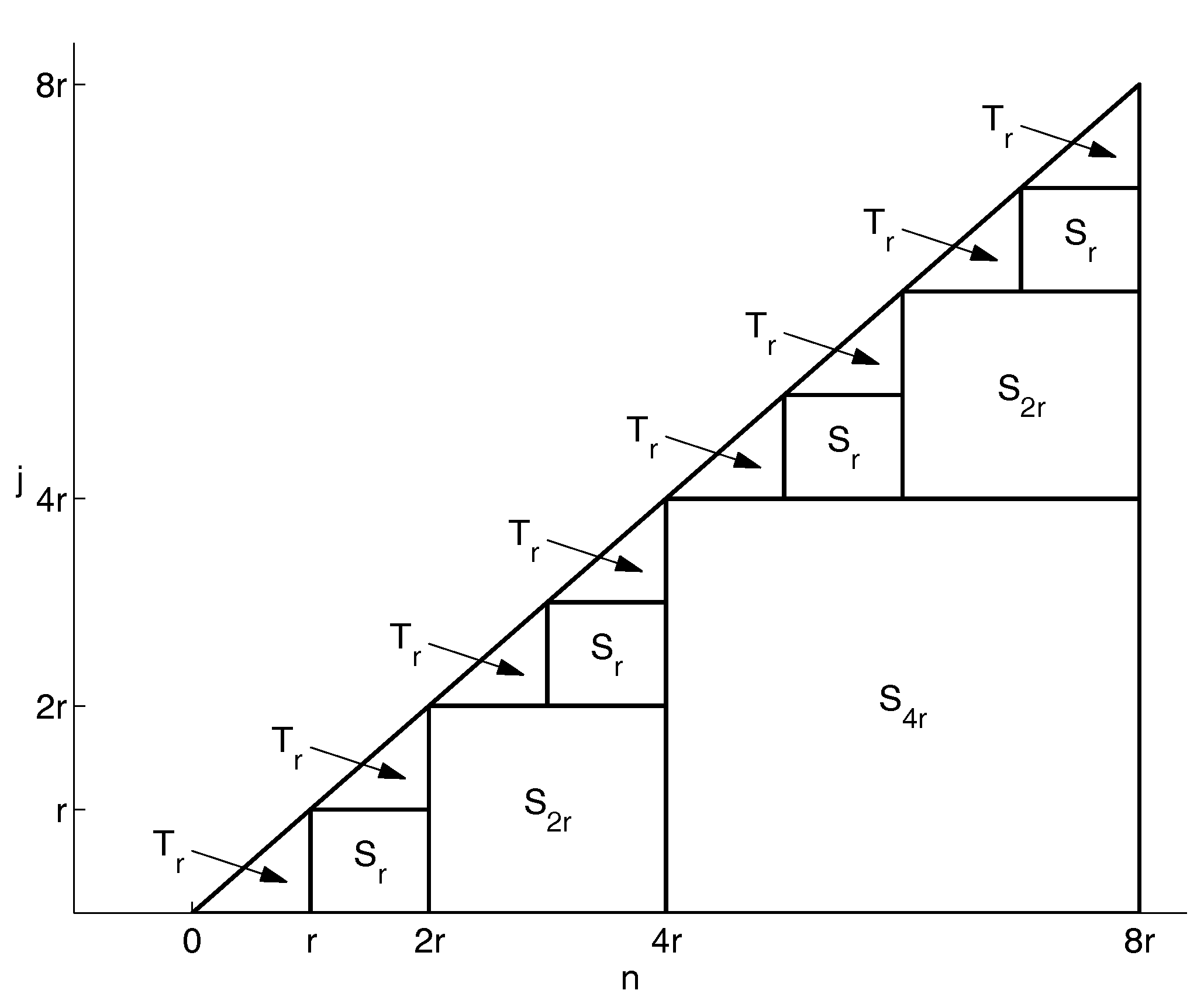
are evaluated in $\mathcal{O}\left(8r{log}_{2}8r\right)$, $\mathcal{O}\left(4r{log}_{2}4r\right)$ and $\mathcal{O}\left(2r{log}_{2}2r\right)$ floating-point operations, respectively. To better understand how this process works, Figure 1 can be of some help, where each square represents the computation of a set of partial sums (by means of the FFT algorithm), and each triangle represents the standard computation of each final convolution term:

$$T_r(p,n)=\sum _{j=p}^n{c}_{n-j}{f}_j,p=\ell r,n\in \{\ell r,\ell r+1,\cdots ,(\ell +1)r-1\},\ell =0,1,2,\cdots .$$

To determine the whole computational cost, we assume, for simplicity, that the total number N of grid points is a power of two. Hence, the computation of one partial sum of length $N/2$ (the square $S_{4r}$ in Figure 1) is requested, involving $\mathcal{O}\left(N{log}_{2}N\right)$ operations, two partial sums of length $N/4$ (the squares $S_{2r}$) each involving $\mathcal{O}\left(\frac{N}{2}{log}_2\frac{N}{2}\right)$ operations, four partial sums of length $N/8$ (the squares $S_r$) each involving $\mathcal{O}\left(\frac{N}{4}{log}_2\frac{N}{4}\right)$ operations, and so on. Additionally, $N/r$ convolution sums of length r (the triangles $T_r$) are requested each with a computational cost proportional to $r(r+1)/2$. Thus, the total amount of computation is proportional to:

$$N{log}_{2}N+2\frac{N}{2}{log}_2\frac{N}{2}+4\frac{N}{4}{log}_2\frac{N}{4}+\cdots +p\frac{N}{p}{log}_2\frac{N}{p}+\frac{N}{r}\frac{r(r+1)}{2},p=\frac{N}{2r},$$

and by means of some simple manipulations, we are able to estimate a computational cost proportional to:

$$\sum _{j=0}^{{log}_{2}p}N{log}_2\frac{N}{2^j}+N\frac{r+1}{2}=\mathcal{O}\left(N{\left({log}_{2}N\right)}^2\right)$$

which, for sufficiently large N, is clearly smaller than $N^2$, i.e., the number of operations required by a computation performed in the standard way.

4. Some Particular Families of FDEs and Systems of FDEs

Equation (6) is perhaps the most standard example of FDEs. The numerical methods presented in the previous sections can be applied both to scalar equations and to systems of FDEs of any size.

There are however other types of fractional-order problems whose treatment necessitates a particular discussion.

4.1. Multi-Order Systems of FDEs

As a special case of non-linear systems of FDEs, we consider systems in which each equation has its own order, which can differ from the order of the other equations. The general form of a MOS of FDEs is:

$$\left\{\begin{array}{c}{D}_{t_0}^{{\alpha }_1}{y}_1\left(t\right)=f_1(t,y\left(t\right))\hfill \\ D_{t_0}^{{\alpha }_2}{y}_2\left(t\right)=f_2(t,y\left(t\right))\hfill \\ ⋮\\ D_{t_0}^{{\alpha }_Q}{y}_Q\left(t\right)=f_Q(t,y\left(t\right))\hfill \end{array}\right.$$

(23)

with $y\left(t\right)=(y_1\left(t\right),\dots ,y_Q\left(t\right))$; it must be coupled with the initial conditions:

$$y\left(t_0\right)=y_0,\frac{\mathrm{d}}{\mathrm{d}t}y\left(t_0\right)=y_0^{\left(1\right)},\cdots ,\frac{{\mathrm{d}}^{m-1}}{\mathrm{d}{t}^{m-1}}y\left(t_0\right)=y_0^{(m-1)},$$

where their number is $m=max\{m_1,m_2,\cdots ,m_Q\}$, with $m_i=⌈{\alpha }_i⌉$, $i=1,2,\cdots ,Q$. Also in this case, it is possible to reformulate each equation of the system (23) in terms of the VIEs:

$$\left\{\begin{array}{c}{\displaystyle y_1\left(t_n\right)=T_{m_1-1}[y_1;t_0]\left(t_n\right)+\frac{1}{\Gamma \left({\alpha }_1\right)}{\int }_{t_0}^{t_n}{(t_n-s)}^{{\alpha }_1-1}{f}_1(s,y\left(s\right))\mathrm{d}s}\hfill \\ {\displaystyle y_2\left(t_n\right)=T_{m_2-1}[y_2;t_0]\left(t_n\right)+\frac{1}{\Gamma \left({\alpha }_2\right)}{\int }_{t_0}^{t_n}{(t_n-s)}^{{\alpha }_2-1}{f}_2(s,y\left(s\right))\mathrm{d}s}\hfill \\ ⋮\hfill \\ {\displaystyle y_Q\left(t_n\right)=T_{m_Q-1}[y_Q;t_0]\left(t_n\right)+\frac{1}{\Gamma \left({\alpha }_Q\right)}{\int }_{t_0}^{t_n}{(t_n-s)}^{{\alpha }_Q-1}{f}_Q(s,y\left(s\right))\mathrm{d}s}\hfill \end{array}\right.$$

(24)

and apply one of the methods described in Section 3.

From the theoretical point of view, there are no particular differences with respect to the solution of a system of FDEs (6) in which all the equations have the same order. The computation is however more expensive due to the need for computing different sequences of weights and evaluating more than one discrete convolution quadrature. It is therefore necessary to optimize the codes to exploit the possible presence of equations having the same order, thus to avoid unnecessary computations; the codes presented in the next section provide this kind of optimization.

4.2. Linear Multi-Term FDEs

A further special case of FDE is when more than one fractional derivative appears in a single equation. Equations of this kind are called multi-term equations, and in the linear case, they are described as:

$${\lambda }_Q{D}_{t_0}^{{\alpha }_Q}y\left(t\right)+{\lambda }_{Q-1}{D}_{t_0}^{{\alpha }_{Q-1}}y\left(t\right)+\cdots +{\lambda }_2{D}_{t_0}^{{\alpha }_2}y\left(t\right)+{\lambda }_1{D}_{t_0}^{{\alpha }_1}y\left(t\right)=f(t,y\left(t\right)),$$

(25)

where ${\lambda }_1,{\lambda }_2,\cdots ,{\lambda }_{Q-1},{\lambda }_Q$ are some (usually real) coefficients and the orders ${\alpha }_1,{\alpha }_2,\cdots ,{\alpha }_{Q-1},{\alpha }_Q$ of the fractional derivatives are assumed (just for convenience) to be sorted in an ascending order, i.e., $0<{\alpha }_1<{\alpha }_2<\cdots <{\alpha }_{Q-1}<{\alpha }_Q$, with ${\lambda }_Q\ne 0$. Note that here we focus on multi-term FDEs, which are linear with respect to the fractional derivatives, but with a (possible) nonlinearity of $f(t,y)$.

The number of initial conditions is given by $m_Q$, where as usual, $m_i=⌈{\alpha }_i⌉$, $i=1,\cdots ,Q$ (and clearly $m_Q=max{m}_i$), and they are expressed in the usual way as derivatives of the solution at the starting point $t_0$:

$$y\left(t_0\right)=y_0,\frac{\mathrm{d}}{\mathrm{d}t}y\left(t_0\right)=y_0^{\left(1\right)},\cdots ,\frac{{\mathrm{d}}^{m_Q-1}}{\mathrm{d}{t}^{m_Q-1}}y\left(t_0\right)=y_0^{(m_Q-1)}.$$

Multi-term FDEs are more difficult to solve than standard FDEs. Anyway, as proposed in [45,46], it is always possible to recast Equation (25) in such a way that some of the methods for FDEs can be easily adapted. Indeed, thanks to Equations (4) and (5) and by applying $J_{t_0}^{{\alpha }_Q}$ to Equation (25), we can reformulate the multi-term FDE as:

$$y\left(t\right)=T_{m_Q-1}[y;t_0]\left(t\right)-\sum _{i=1}^{Q-1}\frac{{\lambda }_i}{{\lambda }_Q}{J}_{t_0}^{{\alpha }_Q-{\alpha }_i}\left[y\left(t\right)-T_{m_i-1}[y;t_0]\left(t\right)\right]+\frac{1}{{\lambda }_Q}{J}_{t_0}^{{\alpha }_Q}f(t,y\left(t\right)).$$

(26)

Hence, numerical methods are straightforwardly devised by applying any method for the discretization of RL integrals (PIs or FLMMs).

As illustrative examples, we consider the generalization of the explicit and implicit first-order PI rules (10) and (11). For this purpose, we first observe that:

$$J_{t_0}^{\alpha }{T}_{m-1}[y;t_0]\left(t\right)=\sum _{k=0}^{m-1}{y}^{\left(k\right)}\left(t_0\right)J_{t_0}^{\alpha }\frac{{(t-t_0)}^k}{k!}=\sum _{k=0}^{m-1}\frac{{(t-t_0)}^{k+\alpha }}{\Gamma (k+\alpha )}{y}^{\left(k\right)}\left(t_0\right)$$

and hence, after denoting:

$$\tilde{T}\left(t\right):=T_{m_Q-1}[y;t_0]\left(t\right)+\sum _{i=1}^{Q-1}\frac{{\lambda }_i}{{\lambda }_Q}\sum _{k=0}^{m_i-1}\frac{{(t-t_0)}^{k+{\alpha }_Q-{\alpha }_i}}{\Gamma (k+{\alpha }_Q-{\alpha }_i+1)}{y}^{\left(k\right)}\left(t_0\right),$$

the corresponding methods for the multiterm FDE (25) are respectively:

$$\mathrm{Expl}.\mathrm{PI}1:y_n=\tilde{T}\left(t\right)-\sum _{i=1}^{Q-1}\frac{{\lambda }_i}{{\lambda }_Q}{h}^{{\alpha }_Q-{\alpha }_i}\sum _{j=0}^{n-1}{b}_{n-j-1}^{({\alpha }_Q-{\alpha }_i)}{y}_j+\frac{1}{{\lambda }_Q}{h}^{{\alpha }_Q}\sum _{j=0}^{n-1}{b}_{n-j-1}^{\left({\alpha }_Q\right)}f(t_j,y_j)$$

(27)

and:

$$\mathrm{Impl}.\mathrm{PI}1:y_n=\tilde{T}\left(t\right)-\sum _{i=1}^{Q-1}\frac{{\lambda }_i}{{\lambda }_Q}{h}^{{\alpha }_Q-{\alpha }_i}\sum _{j=1}^n{b}_{n-j}^{({\alpha }_Q-{\alpha }_i)}{y}_j+\frac{1}{{\lambda }_Q}{h}^{{\alpha }_Q}\sum _{j=1}^n{b}_{n-j}^{\left({\alpha }_Q\right)}f(t_j,y_j).$$

(28)

In a similar way, it is possible to extend to multi-term FDEs also the implicit trapezoidal rule (12):

$$\begin{array}{cc}\hfill \mathrm{Impl}.\mathrm{PI}2:y_n=\tilde{T}\left(t\right)& -\sum _{i=1}^{Q-1}\frac{{\lambda }_i}{{\lambda }_Q}{h}^{{\alpha }_Q-{\alpha }_i}\left({\tilde{a}}_n^{({\alpha }_Q-{\alpha }_i)}{y}_0+\sum _{j=1}^n{a}_{n-j}^{({\alpha }_Q-{\alpha }_i)}{y}_j\right)\hfill \\ & +\frac{1}{{\lambda }_Q}{h}^{{\alpha }_Q}\left({\tilde{a}}_n^{\left({\alpha }_Q\right)}f(t_0,y_0)+\sum _{j=1}^n{a}_{n-j}^{\left({\alpha }_Q\right)}f(t_j,y_j)\right),\hfill \end{array}$$

(29)

which usually assures a higher accuracy; alternatively, in order to avoid the solution, at each step of the nonlinear equations to determine $y_n$ (see the discussion in Section 3.3), also in this case, a predictor-corrector strategy can be of some practical help. Clearly, all these methods apply in a straightforward way to non-scalar problems, as well.

Although several other approaches have been proposed to solve linear multi-term FDEs, we think that the one discussed in this section could be privileged due to its simplicity. The application of FLMMs to Equation (26) is surely possible, but some problems must be solved to properly identify the starting weights on the basis of the behavior analysis of the exact solution; we do not address this problem in this paper.

The computational cost is proportional to Q times the cost of standard PI rules and can be kept under control by applying to each discrete convolution the technique discussed in Section 3.4.

5. MATLAB Routines for Fractional-Order Problems

In this section, we present some MATLAB routines specifically devised to solve fractional-order problems by means of the methods illustrated in this paper. The routines are listed in

Table 2. MATLAB routines for some fractional-order problems. FDEs: fractional differential equations; PI: product-integration.

Name	Problem	Method
FDE_PI1_Ex.m	System of FDEs (6) or (23)	Explicit PI rectangular rule (10)
FDE_PI1_Im.m	System of FDEs (6) or (23)	Implicit PI rectangular rule (11)
FDE_PI2_Im.m	System of FDEs (6) or (23)	Implicit PI trapezoidal rule (12)
FDE_PI12_PC.m	System of FDEs (6) or (23)	Predictor-corrector PI rules (13)
MT_FDE_PI1_Ex.m	Multi-term FDE (25)	Explicit PI rectangular rule (27)
MT_FDE_PI1_Im.m	Multi-term FDE (25)	Implicit PI rectangular rule (28)
MT_FDE_PI2_Im.m	Multi-term FDE (25)	Implicit PI trapezoidal rule (29)
MT_FDE_PI12_PC.m	Multi-term FDE (25)	Predictor-corrector PI rules

with the indicated kind of problem that is aimed to be solved and the specific implemented method.

All the MATLAB routines are available on the software section of the web-page of the author, at the address: https://www.dm.uniba.it/Members/garrappa/Software.

The number 1 in the name of routines based on the PI rectangular rule refers to the convergence order of the underlying formula, while the number 2 stands for the maximum obtainable order (under suitable smoothness assumptions) of the PI trapezoidal rule. For this reason, routines based on PC, which use both PI rectangular rules (as predictor) and PI trapezoidal rules (as corrector), have 1 and 2 in the name. These names have been selected in analogy with the names of some built-in MATLAB functions for ODEs.

The way in which the different routines can be used is quite similar. One of the main differences is in implicit methods, which, in addition to the right-hand side $f(t,y)$, denoted by the function handle f_fun, require also the Jacobian ${\mathbf{J}}_f(t,y)$ of the right-hand side, namely the function handle J_fun; this is necessary to solve the inner nonlinear equation by means of Newton–Raphson iterations as described in Section 3.3.

The routines for solving a standard system of FDEs (6) or an MOS (23) are used by means of the following instructions:

• [t, y] = FDE_PI1_Ex(alpha,f_fun,t0,T,y0,h,param)
• [t, y] = FDE_PI1_Im(alpha,f_fun,J_fun,t0,T,y0,h,param,tol,itmax)
• [t, y] = FDE_PI2_Im(alpha,f_fun,J_fun,t0,T,y0,h,param,tol,itmax)
• [t, y] = FDE_PI12_PC(alpha,f_fun,t0,T,y0,h,param,mu,mu_tol)

Clearly, in case of an MOS, the parameter alpha must be a vector of the same size of the problem, while with a standard system (6), alpha is a scalar value.

Codes for linear multi-term FDEs (25) are used in a slightly different way since they additionally require providing the parameters ${\lambda }_i$, according to:

• [t, y] = MT_FDE_PI1_Ex(alpha,lambda,f_fun,t0,T,y0,h,param)
• [t, y] = MT_FDE_PI1_Im(alpha,lambda,f_fun,J_fun,t0,T,y0,h,param,tol,itmax)
• [t, y] = MT_FDE_PI2_Im(alpha,lambda,f_fun,J_fun,t0,T,y0,h,param,tol,itmax)
• [t, y] = MT_FDE_PI12_PC(alpha,lambda,f_fun,t0,T,y0,h,param,mu,mu_tol)

The meaning of each parameter is explained as follows (note that some of the parameters are optional and can be therefore omitted):

• alpha: order of the fractional derivative; when solving standard systems (6), alpha must be a single scalar value, while with MOSs (23) and linear multi-term FDEs (25), alpha must be a vector;
• lambda: only for linear multi-term FDEs (23), lambda is the vector of the coefficients ${\lambda }_i$ of each derivative in Equation (23);
• f_fun: function defining the right-hand side $f(t,y)$ or $f(t,y,param)$ of the equation; param denotes a possible optional parameter (or a set of parameters collected in a single vector);
• J_fun: Jacobian matrix (or derivative in the scalar case) of the right-hand side $f(t,y)$ of the equation (only for implicit methods) with respect to the second variable y; also, the Jacobian ${\mathbf{J}}_f(t,y)$ can have some parameters, namely ${\mathbf{J}}_f(t,y,param)$;
• t0 and T: initial and final endpoints of the integration interval;
• y0: matrix of the initial conditions with the number of rows equal to the size of the problem and the number of columns equal to the smallest integer greater than $max\{{\alpha }_1,\cdots ,{\alpha }_Q\}$;
• h: step-size for integration; it must be real and positive;
• param: (optional) vector of possible parameters for the evaluation of the vector field $f(t,y)$ and its Jacobian (if not necessary, this vector can be omitted or an empty vector [ ] can be used);
• tol: (optional) fixed tolerance for stopping the Newton–Raphson iterations when solving the internal system of nonlinear equations (only for implicit methods); when not specified, the default value ${10}^{-6}$ is assumed;
• itmax: (optional) maximum number of iterations for the Newton–Raphson method; when not specified, the default value itmax = 100 is used;
• mu: (optional) number of corrector iterations (only for predictor-corrector methods); when not specified, the default value mu = 1 is used;
• mu_tol: (optional) tolerance for testing the convergence of corrector iterations when mu=Inf; when not specified, the default value mu_tol = ${10}^{-6}$ is used.

All the codes give two outputs:

• t: the vector of nodes on the interval $[t_0,T]$ in which the numerical solution is evaluated;
• y: the matrix whose columns are the values of the solution evaluated in the points of t.

6. Some Applicative Examples

In the following, we present some applications of the routines described in the previous section, also in order to show the way in which they can be used.

For problems for which the analytical solution is not known, we will use, as reference solution, the numerical approximation obtained with a tiny step h by the implicit trapezoidal PI rule, which, as we will see, usually shows an excellent accuracy. All the experiments are carried out in MATLAB Ver. 8.3.0.532 (R2014a) on a computer equipped with a CPU Intel i5-7400 at 3.00 GHz running under the operating system Windows 10.

The first test problem aims to show the superiority of implicit methods for stability reasons. For this purpose, we consider the simple linear test equation:

$$y^{\prime }\left(t\right)=\lambda y\left(t\right),y\left(t_0\right)=y_0,$$

(30)

whose exact solution is $y\left(t\right)=E_{\alpha }\left({(t-t_0)}^{\alpha }\lambda \right)$ with:

$$E_{\alpha }\left(z\right)=\sum _{k=0}^{\infty }\frac{z^k}{\Gamma (\alpha k+1)}$$

the Mittag–Leffler function, which can be evaluated thanks to the algorithm described in  [47]. This problem can be solved, in the interval $[0,5]$ and for $\alpha =0.6$ and $\lambda =-10$, by the following few MATLAB lines:

• alpha = 0.6; lambda = -10 ;
• f_fun = @(t,y,lam) lam * y;
• J_fun = @(t,y,lam) lam ;
• param = lambda ;
• t0 = 0 ; T = 5 ; y0 = 1 ; h = 2^(−5) ;

and after calling one of the following routines:

• [t, y] = FDE_PI1_Ex(alpha,f_fun,t0,T,y0,h,param) ;
• [t, y] = FDE_PI1_Im(alpha,f_fun,J_fun,t0,T,y0,h,param) ;
• [t, y] = FDE_PI2_Im(alpha,f_fun,J_fun,t0,T,y0,h,param) ;
• [t, y] = FDE_PI12_PC(alpha,f_fun,t0,T,y0,h,param).

As we can see from the results in

Table 3. Errors and EOC at $T=5.0$ for the FDE (30) with $\alpha =0.6$ and $\lambda =-10.0$.

	PI 1 Expl		PI 1 Impl.		PI 2 Impl.		PI P.C.
h	Error	EOC	Error	EOC	Error	EOC	Error	EOC
$2^{-2}$	7.52(12)		6.80(−4)		5.55(−4)		5.43(21)
$2^{-3}$	3.57(17)	****	3.31(−4)	1.036	1.81(−4)	1.614	2.57(27)	****
$2^{-4}$	8.14(17)	****	1.63(−4)	1.020	5.95(−5)	1.609	7.87(21)	****
$2^{-5}$	1.57(−1)	****	8.11(−5)	1.011	1.95(−5)	1.606	4.22(−4)	****
$2^{-6}$	3.99(−5)	****	4.04(−5)	1.006	6.43(−6)	1.604	3.96(−5)	****
$2^{-7}$	2.00(−5)	0.997	2.01(−5)	1.003	2.12(−6)	1.602	8.90(−6)	2.153
$2^{-8}$	1.00(−5)	0.998	1.01(−5)	1.002	6.98(-7)	1.602	2.43(−6)	1.873

, the explicit methods (including the predictor-corrector, which actually works as an explicit method) provide wrong or inaccurate results for small step-sizes, while implicit methods are able to return reliable results even with large step-sizes (as usual, numbers as $6.38(-6)$ denote $6.38\times {10}^{-6}$). This issue is related to the bounded stability region of explicit methods as already investigated in the paper [29] (see also [48,49]).

In all the tables, we denote with EOC the estimated order of convergence obtained as ${log}_2\left(E\left(h\right)/E(h/2)\right)$, with $E\left(h\right)$ the error corresponding to the step-size h.

For the next test problem, we consider the equation proposed in [25]:

$$D_{t_0}^{\alpha }y\left(t\right)=\frac{40320}{\Gamma (9-\alpha )}{t}^{8-\alpha }-3\frac{\Gamma (5+\alpha /2)}{\Gamma (5-\alpha /2)}{t}^{4-\frac{\alpha }{2}}+\frac{9}{4}\Gamma (\alpha +1)+{\left(\frac{3}{2}{t}^{\frac{\alpha }{2}}-t^4\right)}^3-{\left[y\left(t\right)\right]}^{\frac{3}{2}}$$

(31)

with the exact solution given by $y\left(t\right)=t^8-3t^{4+\frac{\alpha }{2}}+\frac{9}{4}{t}^{\alpha }$. This problem is surely of interest because, unlike several other problems often proposed in the literature, it does not present an artificial smooth solution, which is indeed not realistic in most of the fractional-order applications.

The right-hand side and its Jacobian (for implicit methods), together with the main parameters of the problem, are defined by means of the MATLAB lines:

• f_fun = @(t,y,al) 40320/gamma(9-al)*t.^(8-al) - ...
•  3*gamma(5+al/2)/gamma(5-al/2)*t.^(4-al/2)+9/4*gamma(al+1) + ...
•  (3/2*t.^(al/2)-t.^4).^3 - y.^(3/2) ;
• J_fun = @(t,y,al) -3/2.*y.^(1/2) ;
• alpha = 0.5 ;
• param = alpha ;
• t0 = 0 ; T = 1 ;
• y0 = 0 ;

and the results concerning errors and EOCs are reported in

Table 4. Errors and EOC at $T=1.0$ for the FDE (31) with $\lambda =0.5$.

	PI 1 Expl		PI 1 Impl.		PI 2 Impl.		PI P.C.
h	Error	EOC	Error	EOC	Error	EOC	Error	EOC
$2^{-4}$	8.03(−2)		7.55(−2)		3.71(−3)		3.56(−3)
$2^{-5}$	3.85(−2)	1.060	3.79(−2)	0.997	1.04(−3)	1.842	6.03(−4)	2.560
$2^{-6}$	1.89(−2)	1.025	1.90(−2)	0.998	2.76(−4)	1.907	2.28(−4)	1.407
$2^{-7}$	9.40(−3)	1.009	9.48(−3)	1.000	7.19(−5)	1.941	1.04(−4)	1.135
$2^{-8}$	4.69(−3)	1.002	4.74(−3)	1.001	1.85(−5)	1.961	4.50(−5)	1.204
$2^{-9}$	2.35(−3)	1.000	2.37(−3)	1.001	4.70(−6)	1.974	1.83(−5)	1.294
$2^{-10}$	1.17(−3)	0.999	1.18(−3)	1.002	1.19(−6)	1.982	7.15(−6)	1.359

.

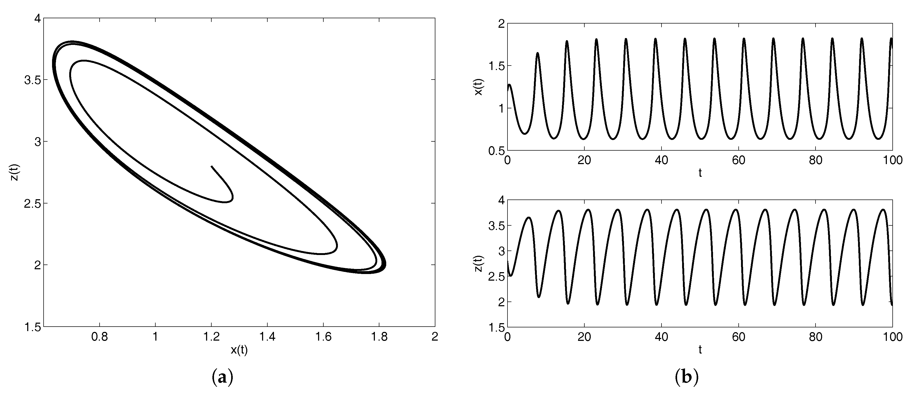
With the aim of showing the application to MOSs of FDEs we first consider a classical fractional-order dynamical system consisting of the nonlinear Brusselator system:

$$\left\{\begin{array}{c}{D}_{t_0}^{{\alpha }_1}x\left(t\right)=A-(B+1)x\left(t\right)+x{\left(t\right)}^{2}z\left(t\right)\hfill \\ D_{t_0}^{{\alpha }_2}z\left(t\right)=Bx\left(t\right)-x{\left(t\right)}^{2}z\left(t\right)\hfill \\ x\left(t_0\right)=x_0,z\left(t_0\right)=z_0,\hfill \end{array}\right.$$

(32)

and we perform the computation for $({\alpha }_1,{\alpha }_2)=(0.8,0.7)$, $(A,B)=(1.0,3.0)$ and $(x_0,z_0)=(1.2,2.8)$ by means of the following MATLAB lines:

• alpha = [0.8,0.7] ;
• A = 1 ; B = 3 ;
• param = [ A , B ] ;
• f_fun = @(t,y,par) [ ...
•   par(1) - (par(2)+1)*y(1) + y(1)^2*y(2) ; ...
•   par(2)*y(1) - y(1)^2*y(2) ] ;
• J_fun = @(t,y,par) [ ...
•   -(par(2)+1) + 2*y(1)*y(2) , y(1)^2 ; ...
•   par(2) - 2*y(1)*y(2) , -y(1)^2 ] ;
• t0 = 0 ; T = 100 ;
• y0 = [ 1.2 ; 2.8] ;

After showing in Figure 2 the behavior of the solution, the errors and the EOCs are presented in

Table 5. Errors and EOC at $T=100.0$ for the Brusselator system of FDEs (32) with $({\alpha }_1,{\alpha }_2)=(0.8,0.7)$, $(A,B)=(1.0,3.0)$ and $(x_0,z_0)=(1.2,2.8)$.

	PI 1 Expl		PI 1 Impl.		PI 2 Impl.		PI P.C.
h	Error	EOC	Error	EOC	Error	EOC	Error	EOC
$2^{-2}$	4.64(−1)		1.03(0)		4.90(−2)		1.16(0)
$2^{-3}$	2.32(−1)	0.996	5.20(−1)	0.988	7.84(−3)	2.643	2.92(−1)	1.994
$2^{-4}$	1.22(−1)	0.926	2.25(−1)	1.211	2.85(−3)	1.460	5.80(−2)	2.333
$2^{-5}$	6.86(−2)	0.834	9.84(−2)	1.191	7.63(−4)	1.903	1.28(−2)	2.179
$2^{-6}$	3.69(−2)	0.896	4.52(−2)	1.124	1.92(−4)	1.991	3.41(−3)	1.910
$2^{-7}$	1.92(−2)	0.941	2.15(−2)	1.071	4.60(−5)	2.060	1.01(−3)	1.758

.

A more involved problem has been considered in [50] as a benchmark problem for testing software for fractional-order problems. It is defined as:

$$\left\{\begin{array}{c}{D}_{t_0}^{0.5}x\left(t\right)=\frac{1}{\sqrt{\pi }}\left(\sqrt[6]{\left(y\right(t)-0.5)\left(z\right(t)-0.3)}+\sqrt{t}\right)\hfill \\ D_{t_0}^{0.2}y\left(t\right)=\Gamma \left(2.2\right)(x\left(t\right)-1)\hfill \\ D_{t_0}^{0.6}z\left(t\right)=\frac{\Gamma \left(2.8\right)}{\Gamma \left(2.2\right)}(y\left(t\right)-0.5)\hfill \\ x\left(0\right)=1,y\left(0\right)=0.5,z\left(0\right)=0.3,\hfill \end{array}\right.$$

(33)

and its analytical solution is $x\left(t\right)=t+1$, $y\left(t\right)=t^{1.2}+0.5$ and $z\left(t\right)=t^{1.8}+0.3$. The results of the evaluation performed on the interval $t\in [0,5]$ by means of the set of MATLAB lines:

• alpha = [0.5, 0.2, 0.6] ;
• f_fun = @(t,y) [ ...
•   (((y(2)-0.5).*(y(3)-0.3)).^(1/6) + sqrt(t))/sqrt(pi) ; ...
•   gamma(2.2)*(y(1)-1) ; ...
•   gamma(2.8)/gamma(2.2)*(y(2)-0.5) ] ;
• J_fun = @(t,y) [ ...
•   0 , (y(2)-0.5).^(-5/6).*(y(3)-0.3).^(1/6)/6/sqrt(pi) , ...
•    (y(2)-0.5).^(1/6).*(y(3)-0.3).^(-5/6)/6/sqrt(pi) ; ...
•   gamma(2.2) , 0 , 0 ; ...
•   0 , gamma(2.8)/gamma(2.2) , 0 ] ;
• t0 = 0 ; T = 5 ;
• y0 = [ 1 ; 0.500000001 ; 0.300000001 ] ;

are presented in

Table 6. Errors and EOC at $T=5.0$ for the MOS of FDEs (33).

	PI 1 Expl		PI 1 Impl.		PI 2 Impl.		PI P.C.
h	Error	EOC	Error	EOC	Error	EOC	Error	EOC
$2^{-2}$	2.56(−1)		1.37(−1)		7.30(−3)		7.84(−2)
$2^{-3}$	1.31(−1)	0.963	7.41(−2)	0.892	3.16(−3)	1.210	3.50(−2)	1.163
$2^{-4}$	6.60(−2)	0.992	3.95(−2)	0.905	1.35(−3)	1.227	1.56(−2)	1.171
$2^{-5}$	3.29(−2)	1.005	2.09(−2)	0.918	5.72(−4)	1.238	6.89(−3)	1.175
$2^{-6}$	1.63(−2)	1.011	1.10(−2)	0.930	2.41(−4)	1.245	3.04(−3)	1.178
$2^{-7}$	8.09(−3)	1.013	5.72(−3)	0.940	1.01(−4)	1.250	1.34(−3)	1.180

where, as suggested in [50], relative errors are evaluated since some of the components of the system rapidly increase.

The main issue with this test equation is related to the presence of a real power in the first equation, which makes the Jacobian of the given function singular at the origin, and hence, it is not possible to apply the Newton–Raphson iterative process in the same way as described in Section 3.3. There are different ways to overcome this issue; for these experiments, we have simply perturbed the initial values by a small amount $\epsilon ={10}^{-8}$; clearly, this perturbation affects the accuracy of the obtained solution, but as we can see from Table 6, where the error is evaluated with respect to the exact solution evaluated with correct initial values, the loss of accuracy is negligible.

Clearly, a comparison of the computational times with those reported in [50] is not possible due to the different features of the computers used for the experiments. Anyway, for the sake of completeness, we report here that with the step-size $h=2^{-7}$, which provides accuracies comparable with those obtained in [50], the execution times (in seconds) of the four MATLAB routines are respectively $0.0369$, $0.0923$, $0.1258$ and $0.0668$.

We conclude this presentation with the multi-term case. As a first test equation, we consider the Bagley–Torvik equation (e.g, see [1]):

$$\left\{\begin{array}{c}{y}^{″}\left(t\right)+a{D}_{t_0}^{3/2}y\left(t\right)+by\left(t\right)=f(t,y\left(t\right)),\hfill \\ y\left(t_0\right)=y_0,y^{\prime }\left(t_0\right)=y_0^{\left(1\right)},\hfill \end{array}\right.$$

(34)

in which, with the aim of showing the robustness of the approaches described in Section 4.2, we have replaced the standard external source $f\left(t\right)$ with a non-linear term $f(t,y(t\left)\right)$ depending on the solution $y\left(t\right)$. On the interval $[0,T]$, we select the parameters $a=2$, $b=\frac{1}{2}$, the initial conditions $y_0=0$ and $y_0^{\left(1\right)}=0$ and the non-linear given function $f(t,y)=t^2-y^{3/2}$. We first show the MATLAB code to set this problem:

• alpha = [2 3/2 0] ;
• lambda = [1 2 1/2] ;
• f_fun = @(t,y) t.^2 - y.^(3/2) ;
• J_fun = @(t,y) -3/2*y.^(1/2) ;
• t0 = 0 ; T = 5 ;
• y0 = [0 , 0 ] ;

and hence, the results of the numerical computation by means of the four codes: problem:

• [t, y] = MT_FDE_PI1_Ex(alpha,lambda,f_fun,t0,T,y0,h)
• [t, y] = MT_FDE_PI1_Im(alpha,lambda,f_fun,J_fun,t0,T,y0,h)
• [t, y] = MT_FDE_PI2_Im(alpha,lambda,f_fun,J_fun,t0,T,y0,h)
• [t, y] = MT_FDE_PI12_PC(alpha,lambda,f_fun,t0,T,y0,h) .

are presented in

Table 7. Errors and EOC at $T=5.0$ for the multi-term FDE (34) with $(a,b)=(2.0,0.5)$, $y\left(0\right)=0$ and $y^{\prime }\left(0\right)=0$.

	PI 1 Expl		PI 1 Impl.		PI 2 Impl.		PI P.C.
h	Error	EOC	Error	EOC	Error	EOC	Error	EOC
$2^{-2}$	3.52(−2)		8.17(−2)		2.72(−4)		8.53(−2)
$2^{-3}$	2.16(−2)	0.704	3.94(−2)	1.053	7.03(−5)	1.950	2.36(−2)	1.855
$2^{-4}$	1.22(−2)	0.826	1.88(−2)	1.067	1.75(−5)	2.005	7.21(−3)	1.709
$2^{-5}$	6.58(−3)	0.888	9.00(−3)	1.063	4.30(−6)	2.026	2.36(−3)	1.609
$2^{-6}$	3.47(−3)	0.925	4.34(−3)	1.052	1.04(−6)	2.046	8.00(−4)	1.564
$2^{-7}$	1.80(−3)	0.948	2.11(−3)	1.041	2.46(-7)	2.082	2.75(−4)	1.540

.

Another interesting example is presented in [50] as the benchmark Problem 2 and consists of the multi-term FDE:

$$\left\{\begin{array}{c}{y}^{‴}\left(t\right)+D_0^{5/2}y\left(t\right)+y^{″}\left(t\right)+4y^{\prime }\left(t\right)+D_0^{1/2}y\left(t\right)+4y\left(t\right)=6cost,\hfill \\ y\left(0\right)=1,y^{\prime }\left(0\right)=1,y^{″}\left(0\right)=-1\hfill \end{array}\right.$$

(35)

whose exact solution is $y\left(t\right)=\sqrt{2}sin(t+\pi /4)$. The MATLAB lines for describing this problem on the interval $[0,100]$ are:

• alpha = [3 2.5 2 1 0.5 0] ;
• lambda = [1 1 1 4 1 4] ;
• f_fun = @(t,y) 6*cos(t) ;
• J_fun = @(t,y) 0 ;
• t0 = 0 ; T = 100 ;
• y0 = [1 , 1, -1 ] ;

and the results obtained by the four MATLAB codes for multi-term FDEs are reported in

Table 8. Errors and EOC at $T=100.0$ for the multi-term FDE (35).

	PI 1 Expl		PI 1 Impl.		PI 2 Impl.		PI P.C.
h	Error	EOC	Error	EOC	Error	EOC	Error	EOC
$2^{-2}$	2.23(−2)		3.07(−2)		1.69(−3)		2.20(−2)
$2^{-3}$	1.03(−2)	1.120	1.34(−2)	1.199	4.04(−4)	2.062	4.35(−3)	2.335
$2^{-4}$	4.33(−3)	1.244	6.16(−3)	1.119	9.84(−5)	2.036	1.24(−3)	1.808
$2^{-5}$	2.29(−3)	0.918	2.92(−3)	1.079	2.42(−5)	2.024	3.98(−4)	1.642
$2^{-6}$	1.20(−3)	0.934	1.40(−3)	1.055	5.97(−6)	2.018	1.34(−4)	1.575
$2^{-7}$	6.18(−4)	0.959	6.84(−4)	1.036	1.50(−6)	1.993	4.58(−5)	1.544

.

In [50], the problem of integrating Equation (35) on the very large integration interval $[0,5000]$ has been discussed. This challenging problem requires a remarkable computational effort, especially when high accuracy is demanded, and in

Table 9. Execution times (in seconds) for solving the multi-term FDE (35) at $T=5000$.

h	N	PI 1 Expl	PI 1 Impl.	PI 2 Impl.	PI P.C.	N (log2N)2
$2^{-2}$	20,000	1.1224	1.8754	1.9601	2.6078	4.08 × 106
$2^{-3}$	40,000	2.0545	3.6506	3.8378	5.1718	9.35 × 106
$2^{-4}$	80,000	4.1367	7.3493	7.6927	10.4410	2.12 × 107
$2^{-5}$	160,000	8.3460	14.7751	15.4799	21.0344	4.78 × 107
$2^{-6}$	320,000	16.9107	29.6091	30.9253	42.3168	1.07 × 108
$2^{-7}$	640,000	34.7736	60.1003	62.8137	86.0035	2.38 × 108

, we have reported the execution times for the same step-sizes h of the previous experiments (in the second column of the table, the corresponding number N of grid-points is also indicated).

We must report that integrating on $[0,5000]$ with small step-sizes by the two methods based on the PI trapezoidal rules leads to some loss of accuracy, while the two methods based only on PI rectangular rules still continue to provide accurate results; this phenomenon, which suggests avoiding the use of PI trapezoidal rules on very large integration intervals, seems related to the accumulation of round-off errors due to the huge number of floating point operations (indeed, the same issue is not reported on smaller integration intervals); as already mentioned in Section 3.4, the number of floating-point operations is proportional to $\mathcal{O}\left(N{\left({log}_{2}N\right)}^2\right)$ (this value is reported in the last column of Table 9), a number that becomes very high in this case.

The propagation of round-off errors for the integration of fractional-order problems on large intervals needs however to be studied in a more in-depth way; as a rule of thumb, in these cases, we just suggest to prefer PI rectangular rules to PI trapezoidal rules due to their better stability properties [29].

7. Conclusions

In this paper we have presented some of the existing methods for numerically solving systems of FDEs and we have discussed their application to multi-order systems and linear multi-term FDEs. In particular, we have focused on the efficient implementation of product integration rules and we have presented some Matlab routines by providing a tutorial guide to their use. Their application has been moreover illustrated in details by means of some examples.

References

- Kilbas, A.A.; Srivastava, H.M.; Trujillo, J.J. Theory and Applications of Fractional Differential Equations; North-Holland Mathematics Studies; Elsevier Science B.V.: Amsterdam, The Netherlands, 2006; Volume 204, p. 523. [Google Scholar]
- Mainardi, F. Fractional Calculus and Waves in Linear Viscoelasticity; Imperial College Press: London, UK, 2010; p. 347. [Google Scholar]
- Miller, K.S.; Ross, B. An Introduction to the Fractional Calculus and Fractional Differential Equations; A Wiley-Interscience Publication, John Wiley & Sons, Inc.: New York, NY, USA, 1993; p. 366. [Google Scholar]
- Podlubny, I. Fractional Differential Equations; Mathematics in Science and Engineering; Academic Press Inc.: San Diego, CA, USA, 1999; Volume 198, p. 340. [Google Scholar]
- Samko, S.G.; Kilbas, A.A.; Marichev, O.I. Fractional Integrals and Derivatives; Gordon and Breach Science Publishers: Yverdon, Switzerland, 1993; p. 976. [Google Scholar]
- Gorenflo, R.; Mainardi, F. Fractional calculus: Integral and differential equations of fractional order. In Fractals and Fractional Calculus in Continuum Mechanics (Udine, 1996); CISM Courses and Lectures; Springer: Vienna, Austria, 1997; Volume 378, pp. 223–276. [Google Scholar]
- Mainardi, F.; Gorenflo, R. Time-fractional derivatives in relaxation processes: A tutorial survey. Fract. Calc. Appl. Anal. 2007, 10, 269–308. [Google Scholar]
- Diethelm, K. The Analysis of Fractional Differential Equations; Lecture Notes in Mathematics; Springer: Berlin, Germany, 2010; Volume 2004, p. 247. [Google Scholar]
- Lubich, C. Runge-Kutta theory for Volterra and Abel integral equations of the second kind. Math. Comput. 1983, 41, 87–102. [Google Scholar] [CrossRef]
- Aceto, L.; Magherini, C.; Novati, P. Fractional convolution quadrature based on generalized Adams methods. Calcolo 2014, 51, 441–463. [Google Scholar] [CrossRef]
- Garrappa, R. Stability-preserving high-order methods for multi-term fractional differential equations. Int. J. Bifurc. Chaos Appl. Sci. Eng. 2012, 22. [Google Scholar] [CrossRef]
- Esmaeili, S. The numerical solution of the Bagley-Torvik by exponential integrators. Sci. Iran. 2017, 24, 2941–2951. [Google Scholar] [CrossRef]
- Garrappa, R.; Popolizio, M. Generalized exponential time differencing methods for fractional order problems. Comput. Math. Appl. 2011, 62, 876–890. [Google Scholar] [CrossRef]
- Zayernouri, M.; Karniadakis, G.E. Fractional spectral collocation method. SIAM J. Sci. Comput. 2014, 36, A40–A62. [Google Scholar] [CrossRef]
- Zayernouri, M.; Karniadakis, G.E. Exponentially accurate spectral and spectral element methods for fractional ODEs. J. Comput. Phys. 2014, 257, 460–480. [Google Scholar] [CrossRef]
- Burrage, K.; Cardone, A.; D’Ambrosio, R.; Paternoster, B. Numerical solution of time fractional diffusion systems. Appl. Numer. Math. 2017, 116, 82–94. [Google Scholar] [CrossRef]
- Garrappa, R.; Moret, I.; Popolizio, M. On the time-fractional Schrödinger equation: Theoretical analysis and numerical solution by matrix Mittag-Leffler functions. Comput. Math. Appl. 2017, 74, 977–992. [Google Scholar] [CrossRef]
- Popolizio, M. A matrix approach for partial differential equations with Riesz space fractional derivatives. Eur. Phys. J. Spec. Top. 2013, 222, 1975–1985. [Google Scholar] [CrossRef]
- Popolizio, M. Numerical approximation of matrix functions for fractional differential equations. Bolletino dell Unione Matematica Italiana 2013, 6, 793–815. [Google Scholar]
- Popolizio, M. Numerical Solution of Multiterm Fractional Differential Equations Using the Matrix Mittag-Leffler Functions. Mathematics 2018, 6, 7. [Google Scholar] [CrossRef]
- Young, A. Approximate product-integration. Proc. R. Soc. Lond. Ser. A 1954, 224, 552–561. [Google Scholar] [CrossRef]
- Lambert, J.D. Numerical Methods for Ordinary Differential Systems; John Wiley & Sons, Ltd.: Chichester, UK, 1991; p. 293. [Google Scholar]
- Dixon, J. On the order of the error in discretization methods for weakly singular second kind Volterra integral equations with nonsmooth solutions. BIT 1985, 25, 624–634. [Google Scholar] [CrossRef]
- Diethelm, K. Smoothness properties of solutions of Caputo-type fractional differential equations. Fract. Calc. Appl. Anal. 2007, 10, 151–160. [Google Scholar]
- Diethelm, K.; Ford, N.J.; Freed, A.D. Detailed error analysis for a fractional Adams method. Numer. Algorithms 2004, 36, 31–52. [Google Scholar] [CrossRef]
- Garrappa, R. Trapezoidal methods for fractional differential equations: theoretical and computational aspects. Math. Comput. Simul. 2015, 110, 96–112. [Google Scholar] [CrossRef]
- Diethelm, K.; Ford, N.J.; Freed, A.D. A predictor-corrector approach for the numerical solution of fractional differential equations. Nonlinear Dyn. 2002, 29, 3–22. [Google Scholar] [CrossRef]
- Diethelm, K. Efficient solution of multi-term fractional differential equations using P(EC)mE methods. Computing 2003, 71, 305–319. [Google Scholar] [CrossRef]
- Garrappa, R. On linear stability of predictor-corrector algorithms for fractional differential equations. Int. J. Comput. Math. 2010, 87, 2281–2290. [Google Scholar] [CrossRef]
- Lubich, C. Discretized fractional calculus. SIAM J. Math. Anal. 1986, 17, 704–719. [Google Scholar] [CrossRef]
- Lubich, C. Convolution quadrature and discretized operational calculus. I. Numer. Math. 1988, 52, 129–145. [Google Scholar] [CrossRef]
- Lubich, C. Convolution quadrature and discretized operational calculus. II. Numer. Math. 1988, 52, 413–425. [Google Scholar] [CrossRef]
- Lubich, C. Convolution quadrature revisited. BIT 2004, 44, 503–514. [Google Scholar] [CrossRef]
- Wolkenfelt, P.H.M. Linear Multistep Methods and the Construction of Quadrature Formulae for Volterra Integral and Integro-Differential Equations; Technical Report NW 76/79; Mathematisch Centrum: Amsterdam, The Netherlands, 1979. [Google Scholar]
- Wolkenfelt, P.H.M. The construction of reducible quadrature rules for Volterra integral and integro-differential equations. IMA J. Numer. Anal. 1982, 2, 131–152. [Google Scholar] [CrossRef]
- Brunner, H.; van der Houwen, P.J. The Numerical Solution of Volterra Equations; CWI Monographs; North-Holland Publishing Co.: Amsterdam, The Netherlands, 1986; Volume 3, p. 588. [Google Scholar]
- Lubich, C. On the stability of linear multi-step methods for Volterra convolution equations. IMA J. Numer. Anal. 1983, 3, 439–465. [Google Scholar] [CrossRef]
- Diethelm, K.; Ford, J.M.; Ford, N.J.; Weilbeer, M. Pitfalls in fast numerical solvers for fractional differential equations. J. Comput. Appl. Math. 2006, 186, 482–503. [Google Scholar] [CrossRef] [Green Version]
- Deng, W. Short memory principle and a predictor-corrector approach for fractional differential equations. J. Comput. Appl. Math. 2007, 206, 174–188. [Google Scholar] [CrossRef]
- Schädle, A.; López-Fernández, M.A.; Lubich, C. Fast and oblivious convolution quadrature. SIAM J. Sci. Comput. 2006, 28, 421–438. [Google Scholar] [CrossRef]
- Aceto, L.; Magherini, C.; Novati, P. On the construction and properties of m-step methods for FDEs. SIAM J. Sci. Comput. 2015, 37, A653–A675. [Google Scholar] [CrossRef] [Green Version]
- Hairer, E.; Lubich, C.; Schlichte, M. Fast numerical solution of nonlinear Volterra convolution equations. SIAM J. Sci. Stat. Comput. 1985, 6, 532–541. [Google Scholar] [CrossRef]
- Hairer, E.; Lubich, C.; Schlichte, M. Fast numerical solution of weakly singular Volterra integral equations. J. Comput. Appl. Math. 1988, 23, 87–98. [Google Scholar] [CrossRef]
- Henrici, P. Fast Fourier methods in computational complex analysis. SIAM Rev. 1979, 21, 481–527. [Google Scholar] [CrossRef]
- Diethelm, K.; Luchko, Y. Numerical solution of linear multi-term initial value problems of fractional order. J. Comput. Anal. Appl. 2004, 6, 243–263. [Google Scholar]
- Nkamnang, A. Diskretisierung von Mehrgliedrigen Abelschen Integralgleichungen und GewöHnlichen Differentialgleichungen Gebrochener Ordnung. Ph.D. Thesis, Freie Universiät Berlin, Berlin, Germany, 1998. [Google Scholar]
- Garrappa, R. Numerical evaluation of two and three parameter Mittag-Leffler functions. SIAM J. Numer. Anal. 2015, 53, 1350–1369. [Google Scholar] [CrossRef]
- Garrappa, R.; Messina, E.; Vecchio, A. Effect of perturbation in the numerical solution of fractional differential equations. Discret. Contin. Dyn. Syst. Ser. B 2018. [Google Scholar] [CrossRef]
- Messina, E.; Vecchio, A. Stability and boundedness of numerical approximations to Volterra integral equations. Appl. Numer. Math. 2017, 116, 230–237. [Google Scholar] [CrossRef]
- Xue, D.; Bai, L. Benchmark problems for Caputo fractional-order ordinary differential equations. Fract. Calc. Appl. Anal. 2017, 20, 1305–1312. [Google Scholar] [CrossRef]
Figure 1.
Scheme of the efficient algorithm for the convolution quadrature (9); squares represent the evaluation of partial sums of length p, and triangles represent convolution sums of fixed length r.
Figure 2.
Behavior of the solution of the Brusselator multi-order system (MOS) (32) in the phase plane (a) and in the and planes (b).