
Greenness as a Differentiating Strategy


Department of Economics, Memorial University of Newfoundland, St. John’s, NL A1C 5S7, Canada
Mathematics 2021, 9(11), 1300; https://0-doi-org.brum.beds.ac.uk/10.3390/math9111300
Submission received: 29 April 2021
/
Revised: 31 May 2021
/
Accepted: 3 June 2021
/
Published: 6 June 2021
(This article belongs to the Special Issue Application of Optimal Control and Game Theory to the Problem of Resource Management)
Abstract
:In a vertical differentiation model, we study a market where consumers, depending on their level of environmental consciousness, value the greenness of the product they consume and are distributed according to a Kumaraswamy distribution. Three scenarios are studied: only one firm takes some green measures and firms compete upon prices; only one firm takes some green measures, and this firm acts as the leader of the price competition; and finally, both firms choose their level of greenness and compete upon their location and price. The results suggest that as consumers become more environmentally conscious, the marginal consumer and the greener firm’s location move to the right. In contrast, the less green firm’s response is non-monotonic. In fact, when the two firms choose their location along with their prices, the latter firm chooses to produce a less green product in response to more environmentally conscious consumers. In the extreme case where all consumers are fully environmentally conscious, the latter firm produces a brown product and sells it at a price equal to its marginal cost. In this case, the greener firm’s price and location choices make the consumers indifferent between the two products. These results could explain why despite all the improvements in the consumers’ environmental consciousness, brown (in its general term) products are still widely produced and consumed, even by environmentally conscious consumers.
1. Introduction
We use the term “green” in its most general meaning, i.e., a green product presents an umbrella of any measures producers take to reflect on any of the consumers’ concerns regarding the environment (more environmentally friendly, more respectful to the environment and animal rights products or more humane alternatives). While the term “brown” is used for a product produced without taking any green measures. Producing a greener product is more costly than producing the brown (basic) alternative and the cost increases exponentially as a firm tries to implement more and more greenness measures. Therefore, firms will be willing to implement a greener procedure only if consumers care about greenness and gain higher satisfaction from consuming greener products, i.e., they are willing to pay higher prices. A look at the trends in the production and consumption habits supports the idea that due to, e.g., environmental awareness and improvement in the living standards, consumers will ask for greener products. However, these factors have different impacts on different consumers depending on their personal preferences, background, income and so on. Thus consumers will remain heterogeneous in terms of their environmental concerns.
This article investigates the impact of consumers’ distribution in terms of their environmental consciousness on the choices of the firms in taking green measures and the prices they charge. Following the literature, e.g., Conrad [1], Anderson et al. [2] and Dixit and Stiglitz [3], we assume each consumer buys only one unit of the product from one of the two firms. There is a continuum of consumers, distributed over the interval, where this interval represents the degree of consumers’ environmental concern. It is also assumed that consumers’ distribution could be presented by a Kumaraswamy distribution of type . The logic behind this choice is that Kumaraswamy distribution is much more general than the uniform distribution which is considered in the standard literature (e.g., see Conrad [1], Dilek et al. [4] among the more recent literature). Indeed, the uniform distribution is nested in the Kumaraswamy distribution when both parameters are set to unity. Moreover, this article contributes to the current literature in terms of model specification as well. We present a new approach in modeling how consumers value and reflect on the greenness of the products they consume by introducing a utility function that better captures the consumers’ environmental consciousness when it comes to the consumption of necessities such as eggs and dairy.
Another novel aspect of this work is that we study and compare three different scenarios. In scenario one, only one firm has access to the resources to produce greener products, while both firms choose their price after this firm has made its choice of greenness level. Since it is assumed that only one firm decides (or has the possibility) to differentiate its product, another possible assumption is that this firm may also act as the leader of the price game (move first). Therefore, scenario two parts from the first scenario by assuming a Stackelberg leader–follower game between the two firms in their price choices. Consideration of these two scenarios is inspired by the real-world observations, where at the beginning of mass production, all products were produced using relatively more pollutive procedures. However, as the pollution problems became more salient, consumers started to demand green products following the green movements and higher income levels. These demands were the driving forces for producers to adopt greener procedures and technologies. However, not all the firms had the means (e.g., the resources and technology) and the will to overcome the inertia of staying with established habits. Therefore, investigating these two scenarios provides valuable insights into understanding this stage of green product evolution. In a third scenario, the assumption that only one firm could move is relaxed, meaning we study a case where both firms can go greener. We assume that the two firms compete with each other by choosing their greenness level and prices in this latter scenario. This scenario coincides with the models presented in the literature.
This article belongs to the literature investigating firms’ strategic interaction when consumers differ in their environmental preferences and awareness. Among many others, e.g., see, Shaked and Sutton [5], Moraga-Gonzalez and Padron-Fumero [6], Ben Elhadj and Tarola [7] for an oligopoly context; see, Ceccantoni et al. [8] for two-country trade examples; and see, Mantovani and Vergari [9,10] for differentiated products along two dimensions, i.e., hedonic quality and environmental quality.
The rest of the paper is organized as follows. Section 2 presents the model set-up. Section 3, Section 4 and Section 5 present the three scenarios and their results. In Section 6, the results of the three scenarios are compared. Concluding remarks are provided in Section 8. All the proofs are presented in Appendix A. Finally, we complete the presentation of our results with a numerical example, presented in Appendix B.
2. Model
Consider a vertical differentiation model, where consumers’ environmental consciousness (producers’ greenness of the products) could be presented on a 0–1 scale, from not conscious to the environmental impacts of the consumption (brown product) to fully conscious (fully green). (As we will see later, in our model the consumers located in origin are indifferent between the two products (cannot differentiate them). Therefore, if we want to be very restrict, the model could be considered as a case of mixed differentiation, which is often lumped with horizontal differentiation in the literature. However, as suggested by one of the referees, since in essence, the greenness feature in our model is about quality and not variety, considering it as vertical differentiation model deemed to be more appropriate). Assume there are two firms, indexed by , and a continuum of consumers that each buys exactly one unit of this product from only one of these producers.
In the early stages of development, consumers are not conscious about the environment, and firms produce an identical brown product, i.e., both firms and consumers are located at the origin in a vertical differentiation model analogy. Many studies support the assumption that consumers are not concerned about the environment at the beginning. Indeed, environmental concern follows awareness, which consumers may not have in the early stages of consuming a product. Moreover, preserving the environment is considered a luxury that will only be demanded when consumers have a high enough economic well-being (see, e.g., [11]). Assuming firms are involved in price competition for their identical product and facing a linear production cost of form , the price for this product, denoted by , is equal to the marginal cost of production, i.e., . The intrinsic utility that a consumer gains from consuming one unit of this product is denoted by . Therefore, consumer j’s net utility from consuming firm i’s product at price , denoted by , at this initial stage is
As consumers receive more information about the environment, animal rights, etc., and their income increases, they begin to become more conscious of the environmental impact of their consumption [11]. However, consumers have different levels of sensitivity to this matter. Assuming consumers are spread over the interval, we can interpret consumer j’s distance from the origin, , as the relative value (or the ratio) that she puts on the greenness of the product she consumes. That means if a consumer is at the origin, they give no value to the greenness, while a consumer on any point is partially conscious and places some value on it, and the extreme environmentalist is located at point 1 and gives a value of 1 to the greenness of the product she consumes. In other words, buying a relatively greener product gives higher satisfaction (by making her feel good about herself and the proper choice that she has made, for example) to a more conscious consumer. Necessities, such as milk or eggs that consumers typically have in their daily consumption, but some consumers might be willing to, for example, pay more to get free-run eggs or free-range chicken, are neat examples matching this description. As one can see from these examples, the greenness of a product in this context is more about a consumer’s perception rather than the actual environmental impacts of the products. This assumption coincides with the fact that consumers are, to some extent, willing to pay higher prices for what they perceive as a greener product, but if the price is too high, they may switch to a brown alternative.
A producer becoming greener means moving from the origin to a new point, , in the interval . Analogous to the consumers’ preferences, the further a firm relocates from the origin, the greener its product is. To capture the proposed consumers’ valuation over their consumption, we can present consumer j’s extra utility from consumption of firm i’s product by a multiplicative function of the form . It is worth mentioning that here, we are parting from the current literature in order to make our model more realistic and to better represent the fact that consumers may gain satisfaction from consuming a product that they perceive as greener (regardless of the actual environmental impact of the product) based on their environmental consciousness, as explained in the introduction. Therefore, the consumer net utility from buying one unit of firm i’s product at the price is
Assume that the consumers’ distribution can be presented by a Kumaraswamy distribution with the following density and cumulative functions:
where represents consumers’ location, and a and b are non-negative shape parameters of the distribution. The logic behind this choice is that the Kumaraswamy distribution is very similar to the Beta distribution; therefore, it can represent a large variety of shapes. However, it has a great advantage over Beta distribution due to its closed-form cumulative distribution function [12]. Moreover, the uniform distribution, which has been widely applied in the literature of product differentiation, is just a specific case of this distribution when a and b are both set to unity. To find the explicit solutions for the model, the parameter b is set to unity in this article. Note that while this simplifying assumption removes some specific shapes of the distribution, it still can cover a variety of shapes. Table 1 summarizes the shapes that this distribution can take after setting parameter b as unity.
In what follows, three different cases are studied. First, it is assumed that only one firm, namely Firm 2, can/has the will to locate at a different point other than the origin, i.e., take greenness measures. This assumption coincides with situations that only one firm has access to the resources or the new technologies and/or has the will to go through a change. In the real-world, firms may simply choose to stay with established habits and not take any greenness measures due to inertia or the transaction costs. Two different scenarios under this assumption are investigated. In the first scenario, which for simplicity is called the Nash competition, firms compete as Nash–Cournot competitors over their price. The second scenario, called Stackelberg competition for simplicity, looks into the case where Firm 2 acts as the leader in the price competition game. Finally, the assumption that only one firm chooses its location is relaxed, and we investigate the case where both firms decide upon their level of greenness while they compete against each other by choosing both price and location. We call this latter case Cournot competition for simplicity.
3. Only One Green Firm: Nash Competition
Without loss of generality, suppose that Firm 2 is the one that has the means and/or the will to improve its production procedure and becomes (partially or fully) green. In a vertical differentiation model analogy, Firm 2 can differentiate its product from Firm 1 by relocating and moving to the location . Suppose that relocation cost has the standard quadratic form of , where r is a positive constant.
A consumer’s satisfaction depends on how much she cares about greenness, how green the consumed product is and how much she pays for the product. Specifically, consumer j’s utility from consuming Firm 2’s product is as follows: and from firm 1’s product is , since . To define the market shares of the two firms, we compute the “marginal consumer”, i.e., the consumer is indifferent between purchasing a product from Firm 1 and 2, for given pairs of prices and products Neven [13]. This consumer’s location, x, satisfies . Therefore, we have the following:
x defines how the market is divided between the two firms: all consumers located on its right-hand-side, i.e., on the interval , will choose Firm 2; those located on its left-hand-side, i.e., on the interval , will choose Firm 1; and consumers at x are indifferent between the two. (As usual, it is assumed that each consumer buys only one unit of only one of the two products and not both).
The two firms are aiming at maximizing their profits. In the current scenario, Firm 2 has two choices: location, —how greener becomes—and its price, , while Firm 1 is located at the origin and only chooses its price. Therefore, Firm 2’s problem is as follows:
subject to (5) and taking as given. Firm 1’s problem is
subject to (5) and taking and as given.
The results are subscripted by n and presented in Proposition 1.
Proposition 1.
Assuming an internal solution exists, if only Firm 2 produces a greener product and the two firms compete over prices, then the location of Firm 2, the marginal consumer and prices are as follows:
Proof.
See Appendix A.1. □
Proposition 1 suggests that more environmentally conscious consumers, i.e., larger a, incentivizes Firm 2 to produce a greener product and sell it at a higher price. Another interesting result is that, as long as a remains small, specifically, for , an increase in environmental consciousness of consumers leads to a higher price for the brown product as well, i.e., . However, after a threshold, this relationship inverses, and as consumers become more and more conscious, the brown product’s price falls. Note, when , consumers are concentrated near the origin (a monotonically decreasing PDF) and when , the majority of consumers are concentrated near 1. Nevertheless, the brown product price decreases only when the concentration of consumers near 1 passes the threshold of . This result suggests that at the early stages, consumers begin to demand greener products, this could result in a higher price for the brown product as long as a large portion of the consumers yield a relatively small value to the products’ greenness. However, the difference between the two prices, , always increases in a.
The impact of the relocation cost on firms’ choice variables is as expected. Indeed, higher relocation cost reduces the greenness level of Firm 2’s product, i.e., , and consequently, by reducing the difference between the two products, a higher relocation cost reduces the two prices, i.e., . The difference between the two prices decreases in r, meaning the impact of relocation cost is stronger for Firm 2, as expected. Corollary 1 summarizes these results.
Corollary 1.
For all , the marginal consumer’s location and Firm 2’s location and price increase in a, since . Firm 1’s price is increasing in a for small values of a and decreasing for large a, in particular only for and otherwise. The distance between the two prices increases in a, .
Firm 2’s location and both firms’ prices are decreasing in relocation cost, . However, .
4. Only One Green Firm: Stackelberg Competition
This section investigates the case where the firm that produces the greener product, Firm 2, moves first in making their choices; in other words, it acts as the Stackelberg leader. For simplicity, we call this case the Stackelberg competition, and the results are subscripted by . Since Firm 1 makes its choice of price by taking Firm 2’s price and location as given, Firm 1’s problem remains as before and, its reaction function is given by (A7). Thus, given (6) and (A7), leader’s first-order conditions are as follows:
Proposition 2 presents the results.
Proposition 2.
Assuming an internal solution exists (and ), if Firm 2 is the only firm that produces a relatively green product and acts as the leader of the game, then Firm 2’s location, the marginal consumer, and prices are as follows:
Proof.
See Appendix A.2. □
As expected, the impact of r on Firm 2’s location, the indifferent consumer, and prices remains the same. The impact of a on firm 2’s location and the indifferent consumer also remains the same as in the previous case. However, unlike the Nash game, when Player 2 acts as the Stackelberg leader, Firm 1’s price always declines as consumers become more environmentally conscious, i.e., and firm 2 raises its price only when consumers’ environmental concerns pass a threshold of . Indeed, by exploiting its first-mover advantage, Firm 2 reduces its price when consumers are mostly concentrated near the origin, and consequently, tries to take a higher share of the market. In response, Firm 1 will lower its price as well. However, as more consumers lean to the right, Firm 2 seizes the opportunity to increase its price, while Firm 1 needs to drop its price further to attract now farther away consumers. As before, the distance between the two prices, , is increasing in a and decreasing in r. Corollary 2 presents this formally.
Corollary 2.
For all , Firm 2’s and the marginal consumer’s location are increasing in a, since and Firm 1’s price is decreasing in a, . Firm 2’s price responds to a change in a non-monotonically, such that only when . The distance between the two prices increases in a, .
Both prices and locations are decreasing in relocation cost, and also .
Another noteworthy characteristic of the solution, in this case, is that for extremely small values of a, the prices suggested by the in Proposition 2 will be unreasonably high. Indeed, (). That is why in the proposition, we rule out the cases of extremely small values of a. When consumers are concentrated at the origin, the leader cannot effectively practice its first-mover advantage. Consequently, for , the solution to the above problem is a corner solution where both firms remain at the origin and charge a price equal to the marginal cost, i.e., the Bertrand competition will prevail. The numerical examples provided in Appendix B shed more light on this case
5. Cournot Competition
This section investigates the standard case where both firms decide (and have the means and the will) to make their product greener, i.e., choose their location and price. The assumption here is that the two firms compete against each other, and the results are subscripted by c. Without loss of generality, let’s assume Firm 2’s product is, at least, as green as Firm 1’s, i.e., Firm 2 is located on or the right-hand side of Firm 1’s location.
A consumer located at is indifferent between the two firms if she gains the same level of satisfaction from buying either of the two products, i.e., the following condition holds:
This leads to the following market division condition:
Proposition 3 summarizes the solution.
Proposition 3.
Assuming an internal solution exists, if both firms decide upon their location and price as competitors then the location of the two firms, the marginal consumer, and the prices are as follows:
Proof.
See Appendix A.3. □
As expected, Firm 2 will be located further away and charges a higher price when consumers are more environmentally conscious. However, Firm 1’s behavior is non-monotone, indeed only when a is small, Firm 1 increases its price and is located further away in response to an increase in a, while when a is large ( for location and for price), Firm 1 responds to a further increase in a by coming closer to the origin and lowering its price. As so, in the extreme case of fully environmentally conscious consumers (), Firm 1 chooses to produce a brown product—located at the origin—and sell its product at its marginal cost c, while Firm 2 is located at , assuming (at 1 otherwise), and charges a price of , assuming . Under these circumstances, consumers remain indifferent between the two products, and one can assume that the market will be equally shared between the two firms. In other words, in the extreme case of fully environmentally conscious consumers, we face a dilemma where one firm chooses to take no green measures at all, and half of the consumers continue to consume that product. The difference between the two prices and locations is increasing in a and decreasing in r. Indeed, the impact of r remains the same as in previous cases. These results are formally presented in Corollary 3.
Corollary 3.
For all , Firm 2’s location and price, and marginal consumer’s location increase in a, i.e., . Only for we have and for we have . The distance between the two prices and locations is increasing in a, , , with and .
Both prices and locations are decreasing in r, i.e., and also , .
6. Comparison
From comparing the results in these different scenarios, the first noteworthy observation is that even if only one of the firms takes some green measurements, the resulted product differentiation gives the firm with brown product some market power. As a result, this firm will be able to raise its price above the marginal cost or the competitive price. The increase in the brown product price depends non-monotonically on consumers’ environmental consciousness level and inversely on the relocation cost. In fact, the relocation cost defines the level of differentiation between the two products—the firms’ distance from each other.
Comparison of the results in Propositions 1 to 3 reveals that the Stackelberg assumption leads to the production of the greenest product when compared to the other two scenarios (); however, since this product is sold at a higher price than the green product in other scenarios () fewer consumers end-up buying it (). Moreover, when only one firm relocates, the price for the brown product is higher than the less green product in the scenario when both firms relocate (). Meaning, when Firm 1 takes no greenness measures, its consumers end up buying a brown product and pay more for it than the case it takes some greenness measures. Comparing the Cournot scenario with Nash scenario reveals that the but and such that at the end, the marginal consumer remains the same in both scenarios, i.e., . Proposition 4 summarizes these results.
Proposition 4.
Firms’ location and prices and the marginal consumer under different scenarios compare as follows:
- .
- .
- .
- .
For extreme values, meaning when all consumers are located at the origin () and when all consumers are located at 1 (), the results are as expected. Indeed, when , in all cases, both firms are located at the origin and charge a price equal to the marginal cost. For the other extreme case of , Firm 1 is located at the origin and charges marginal cost as its price, while Firm 2 is located at the and imposes a price equal to which will make consumers indifferent between the two products.
7. Alternative Timing Scenarios
In the above analysis, we assumed that the location (quality) choice happens simultaneously with the price choice (only for Firm 2 in the first two cases and for both firms for the last case). Intuitively, up to here (except for the Stackelberg case), we are assuming that firms could effectively hide their location (quality) and price choices from each other. Therefore, the simultaneous assumption reflects the lack of information about the choice of the other firm and not necessarily their simultaneous move. In the Stackelberg competition case, we also assume that the leader launches its product quality and price first, and then the follower chooses its price after observing the choices made by the leader. Alternatively, one can assume that firms observe each other’s location before making their price choices. This assumption will separate the location choice stage from the price choice stage, where the latter happens at the final stage. Consideration of this alternative timing leads to fascinating results. Indeed, under such assumption, Firm 1’s optimal choice is always producing the brown product, i.e., taking no green measures. This happens because, by design, if we separate the price competition stage from the quality competition, the location of the indifferent consumer will be defined as a constant in that stage and will always be equal to . Therefore, Firm 1’s profit becomes strictly decreasing in its location. Proposition 5 reports this result.
Proposition 5.
Assuming an internal solution exists, if both firms decide upon their price after the location choices are made, then staying at the origin is the optimal choice for Firm 1. The indifferent consumer’s location is , while the location of Firm 2 and the prices are as follows:
Under the Stackelberg assumption:
Under the Cournot assumption:
As we can see from Proposition 5, the qualitative analysis we provided before regarding the prices and Firm 2’s location remains valid under this alternative timing as well.
8. Concluding Remarks
In a vertical differentiation model, we study a market where consumers, depending on their level of environmental consciousness, value the greenness of the product they consume. We assume that consumers’ environmental consciousness distribution could be presented by a Kumaraswamy distribution of type . We investigate the firms’ choices for the price and location under three different scenarios. At first, we study a situation where only one of the firms has the means (technology, resources, etc.) to take some green measures in its production procedures. We study two different scenarios under this condition: when the two firms play as Cournot competitors and when the greener firm acts as the Stackelberg leader. To complete the discussion, we investigate the standard case when both firms choose their location and price and act as Cournot competitors.
Our analysis shows that as consumers become more environmentally conscious in all three scenarios, the marginal consumer’s and Firm 2’s (the greener firm’s) location move to the right. Moreover, in the first and last scenario, Firm 2 charges a higher price for its now greener product as a increases. However, when Firm 1 continues to produce the brown product and Firm 2 acts as the Stackelberg leader, the latter increases its price in response to an increase in consumers’ environmental consciousness only if a is large. Firm 1’s response to a change in a differs from case to case, and it is mostly non-monotone; however, in all cases when a is large, Firm 1 responds to a further increase in this parameter by dropping its price. In all cases, the distance between the two prices increases as consumers become more environmentally conscious. Intuitively, firms differentiate to soften competition. Thus, when Firm 2 becomes greener (the farther from the origin it is located), the two products will no longer be perfect substitutes. Indeed, by moving away from zero, Firm 2 increases the willingness to pay for all consumers, and therefore, can charge a higher price. Nevertheless, as this firm raises her price, Firm 1 can follow as long as they can attract some consumers (this is so when a is smaller than a threshold, depending on the case). Otherwise, she has to lower the price as few consumers are close to zero, in such situation, lowering the price is the only viable way to compete.
When the two firms can choose their location and prices, a surprising observation is that only one of the firms continues to improve their product’s greenness when consumers become more and more environmentally conscious. In contrast, the other chooses to produce a less green product. So much so, in the extreme case that all consumers give a value of one to the greenness of the product, the latter firm produces a brown product and sells it at a price equal to the marginal cost. In this situation, the greener firm’s price and location choices make the consumers indifferent between its product and the brown product. These results could explain why despite all the improvements in the consumers’ environmental consciousness, we still observe that brown (in its general term) products are widely produced and consumed, even by the environmentally-conscious consumers! This also suggests that to move toward greener products, some market interference is necessary.
To complete our analysis, we also investigated the case where the price decision happens after firms observe the location (quality) choices. The fascinating result in this case is that the optimal choice for one of the firms will always be to take no greenness measures and produce a fully brown product.
We acknowledge that there are many valuable and interesting avenues in this current work. First of all, the focus here is only on the consumers’ perception of the greenness of the product they consume. As we know, this perception may or may not match the actual environmental impact of that product. For example, while cage-free eggs are considered a greener product by consumers, in a study of environmental impacts of egg production, Xin et al. [14] conclude that non-cage houses cause lower efficiency in resource (feed, energy, and land) utilization, leading to a more significant carbon footprint. Therefore, extending the current model to embed the social-environmental impact of the products would be very insightful. It will also be exciting to extend this model to a case where firms can affect the consumers’ views and their level of consciousness by, for example, advertising. Finally, an obvious invaluable extension would be making the model dynamic to capture how firms’ and consumers’ choices change over time.
Funding
This research received no external funding.
Institutional Review Board Statement
Not applicable.
Informed Consent Statement
Not applicable.
Data Availability Statement
No new data were created or analyzed in this study. Data sharing is not applicable to this article.
Conflicts of Interest
The author declares no conflict of interest.
Appendix A. Technical Appendix
Appendix A.1. Proof of Proposition 1
By rearranging (A2) we have the following:
Rearrangement of (A1) yields
Combining these two defines Firm 2’s price implicitly as follows:
Given problem (7), Firm 1’s first-order-condition is
By replacing by (5) and then rearranging the above condition we have the following:
Replacing the prices into (A3) yields
Finally, the marginal consumer is
These complete the proof.
Note that is always increasing in and for we have and . Therefore, the sufficient condition for having internal solution, or , is , when and otherwise.
Appendix A.2. Proof of Proposition 2
From (A7) we have
Substituting in (A10) results in the following:
Finally, by replacing and in (A8), we obtain the result for and substituting that in (5) completes the proof.
Note, since is always increasing in and for , we have and . Therefore, the sufficient condition for is when and otherwise.
Appendix A.3. Proof of Proposition 3
Firm 1’s problem is the following:
Thus, the first-order conditions are
Thus, the first-order conditions are
Using it in (A19) yields
Substituting in (A21) and (A22), completes the results for and , respectively. Then, we can easily solve for the rest, e.g., by substituting these results in (A16) to first solve for and use (14) to find .
Note that is always increasing in and for , we have and . Therefore, the sufficient condition for is , when and otherwise.
Appendix B. Numerical Illustrations
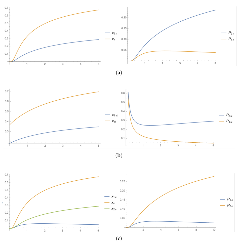
To shed more light on the behavior of firms’ choices and the indifferent consumer’s location under different scenarios, here we provide a numerical example. In this example, without loss of generality, we normalize r to unity. From this figure, we can see that in most cases when , Firm 2’s location and price could be fuzzy, and only for values of a—level of consumers’ environmental concerns—beyond a minimum threshold which makes taking green measures economically viable, Firm 2’s behavior is nicely defined and follows the trends as expected. As explained in Section 4 and it is obvious from Figure A1b, right panel, the fuzzy behavior of Firm 2’s price is more apparent in the case when this firm acts as the leader of the game.
Figure A1.
Left panels present the locations and right panels present the variable part of the prices (i.e., ). (a) Nash competition; (b) Stackelberg competition; (c) Cournot competition.
Figure A1.
Left panels present the locations and right panels present the variable part of the prices (i.e., ). (a) Nash competition; (b) Stackelberg competition; (c) Cournot competition.

References
- Conrad, K. Price Competition and Product Differentiation When Consumers Care for the Environment. Environ. Resour. Econ. 2005, 31, 1–19. [Google Scholar] [CrossRef]
- Anderson, S.P.; Palma, A.D.; Thisse, J.F. Demand for Differentiated Products, Discrete Choice Models, and the Characteristics Approach. Rev. Econ. Stud. 1989, 56, 12–35. [Google Scholar] [CrossRef]
- Dixit, A.K.; Stiglitz, J.E. Monopolistic Competition and Optimum Product Diversity. Am. Econ. Rev. 1977, 67, 297–308. [Google Scholar]
- Dilek, H.; Karaer, Ö.; Nadar, E. Retail location competition under carbon penalty. Eur. J. Oper. Res. 2018, 1, 146–158. [Google Scholar] [CrossRef] [Green Version]
- Shaked, A.; Sutton, J. Relaxing price competition through product differentiation. Rev. Econ. Stud. 1982, 49, 3–13. [Google Scholar] [CrossRef]
- Moraga-Gonzalez, J.; Padron-Fumero, N. Environmental policy in a green market. Environ. Resour. Econ. 2002, 22, 419–447. [Google Scholar] [CrossRef]
- Ben Elhadj, N.; Tarola, O. Relative quality-related (dis)utility in vertically differentiated oligopoly with an environmental externality. Environ. Dev. Econ. 2015, 20, 354–379. [Google Scholar] [CrossRef] [Green Version]
- Ceccantoni, G.; Tarola, O.; Zanaj, S. Green Consumption and Relative Preferences in a Vertically Differentiated International Oligopoly. Ecol. Econ. 2018, 149, 129–139. [Google Scholar] [CrossRef] [Green Version]
- Mantovani, A.; Tarola, O.; Vergari, C. Relative quality-related (dis)utility in vertically differentiated oligopoly with an environmental externality. Resour. Energy Econ. 2016, 45, 99–123. [Google Scholar] [CrossRef]
- Mantovani, A.; Vergari, C. Environmental vs hedonic quality: Which policy can help in lowering pollution emissions? Environ. Dev. Econ. 2017, 22, 274–304. [Google Scholar] [CrossRef] [Green Version]
- Diekmann, A.; Franzen, A. The Wealth of Nations and Environmental Concern. Environ. Behav. 1991, 31, 540–549. [Google Scholar] [CrossRef]
- Mitnik, P.A. New properties of the kumaraswamy distribution. Commun. Stat. Theory Methods 2013, 42, 741–755. [Google Scholar] [CrossRef]
- Neven, D. Two Stage (Perfect) Equilibrium in Hotelling’s Model. J. Ind. Econ. 1985, 33, 317–325. [Google Scholar] [CrossRef]
- Xin, H.; Gates, R.; Green, A.; Mitloehner, F.; Moore, P.; Wathes, C. Environmental impacts and sustainability of egg production systems. Poult. Sci. 2011, 90, 263–277. [Google Scholar] [CrossRef] [PubMed]

Table 1.
Characteristics of the Kumaraswamy distribution for different parameter values [12].
Table 1.
Characteristics of the Kumaraswamy distribution for different parameter values [12].
Publisher’s Note: MDPI stays neutral with regard to jurisdictional claims in published maps and institutional affiliations. |
© 2021 by the author. Licensee MDPI, Basel, Switzerland. This article is an open access article distributed under the terms and conditions of the Creative Commons Attribution (CC BY) license (https://creativecommons.org/licenses/by/4.0/).
Share and Cite
MDPI and ACS Style
Masoudi, N. Greenness as a Differentiating Strategy. Mathematics 2021, 9, 1300. https://0-doi-org.brum.beds.ac.uk/10.3390/math9111300
AMA Style
Masoudi N. Greenness as a Differentiating Strategy. Mathematics. 2021; 9(11):1300. https://0-doi-org.brum.beds.ac.uk/10.3390/math9111300
Chicago/Turabian StyleMasoudi, Nahid. 2021. "Greenness as a Differentiating Strategy" Mathematics 9, no. 11: 1300. https://0-doi-org.brum.beds.ac.uk/10.3390/math9111300
Note that from the first issue of 2016, this journal uses article numbers instead of page numbers. See further details here.