On the Stability of Convection in a Non-Newtonian Vertical Fluid Layer in the Presence of Gold Nanoparticles: Drug Agent for Thermotherapy

Abstract

We consider the effect of gold nanoparticles on the stability properties of convection in a vertical fluid layer saturated by a Jeffreys fluid. The vertical boundaries are rigid and hold at uniform but different temperatures. Brownian diffusion and thermophoresis effects are considered. Due to numerous applications in the biomedical industry, such a study is essential. The linear stability is investigated through the normal mode disturbances. The resulting stability problem is an eighth-order ordinary differential complex eigenvalue problem that is solved numerically using the Chebyshev collection method. Its solution provides the neutral stability curves, defining the threshold of linear instability, and the critical parameters at the onset of instability are determined for various values of control parameters. The results for Newtonian fluid and second-grade fluid are delineated as particular cases from the present study. It is shown that the Newtonian fluid has a more stabilizing effect than the second-grade and the Jeffreys fluids in the presence of gold nanoparticles and, Jeffreys fluid is the least stable.

1. Introduction

Nanofluid is visualized to describe a fluid in which nanometer-sized particles (10–100 nm) are stably suspended in conventional heat transfer basic fluids. Most materials used for nanoparticles contain oxides such as alumina, silica, titania, and copper oxide, and metals such as copper and gold. Gold nanoparticles (GNPs) are essential in biomedical sciences and emerge as promising agents for treatment. For a prolonged period, diseases such as cancer, gland tumors, and arthritis were considered incurable. Notably, malignant growth is perhaps the biggest hindrance among infection that mankind can experience. Specialists are bending over backward to kill this illness. As of late, nanoparticles have been taken to the front line of malignancy research due to their moderately enormous surface zone and blend balance, solid tunability, and expanded optical properties. Yet, because of the benevolent and untiring endeavors of researchers, scientific experts, and specialists, a cure is no longer a fantasy. Presently, there are intense medications and medications accessible to dispose of them. Moreover, the development of new and refined mechanical assemblies in clinical sciences caused specialists to feel certain that they were striking enough to play out some basic tasks and medical procedures. The equivalent applies to censure tissues and malignancy present in the human body without settling on the decision of analyzing parts or organs. Infiltration of nano-size gold particles through catheters conveying the necessary medications to the harmed organs has shown surprising outcomes. A modeling study on heated couple-stress fluid peristaltically conveying gold nanoparticles through coaxial tubes was investigated by Hussain et al. [1]. The peristaltic blood flow with gold nanoparticles as a third-grade nanofluid in a catheter was studied by Mekheimer et al. [2]. Many authors analyzed the mechanism of nanofluids with the application of peristaltic flow [3,4,5,6,7]. For the last few decades, several authors have analyzed the stability of the flow in vertical channels, where their works concern the hydrodynamic stability of pure fluids [8,9,10,11].

Moreover, there are some research works concerning the flow of nanofluids: Lin et al. [12] for the nanofluids stability in a channel flow, Xia and Lin [13] for the flow instability of nanofluids in jet, Anuar et al. [14] for the MHD stability of flow past a nonlinear stretching/shrinking sheet in carbon nanotubes, and Hussain et al. [15] for linear MHD instability of Hartmann flow with nanoparticles Fe₂O₃ in water. Among many types of nanoparticles, gold nanoparticles (GNPs) have been used to treat cancer as a result of effects of their quantum size and their large surface area compared with other metal atoms in addition to their ability to absorb energy. Consequently, the use of gold nanoparticles in a wide variety of applications seems advantageous, the only disadvantages so far being their high price.

The unsteadiness component of the convective stream happens because of the energy move from the fundamental stream to the speed annoyances, compared to the presence of warm modes. Additionally, for the convective stream, the unsteady separation of the medium emerges as a result of warming. The insecurity happens because of the impact of thickness, temperature, and gravity inhomogeneities. In this way, there exists collaboration between the warm insecurity and the hydrodynamic annoyances which entangle the issues. A significant number of the base liquids show viscoelastic conduct and consequently considering the viscoelastic model is more proper than an inelastic sort of non-Newtonian model in the investigation of warm convective insecurity in nanofluids. By and large, viscoelastic insecurity is seen in polymer dissolves just as in polymer arrangements. Many researchers have studied the stability of convection in a vertical fluid layer by considering various non-Newtonian effects [16,17,18,19,20,21].

The present paper intends to study the simultaneous presence of radiation and chemical reaction on the stability of convection of the Jeffreys fluid model [22,23] with gold nanoparticles in a vertical fluid layer. The system of partial differential equations that describes this model with subjected boundary conditions is transformed to an ordinary differential eigenvalue problem and solved numerically by using the Chebyshev collocation method. The effect of the relevant parameters on the stability characteristics is numerically discussed with the help of illustrations.

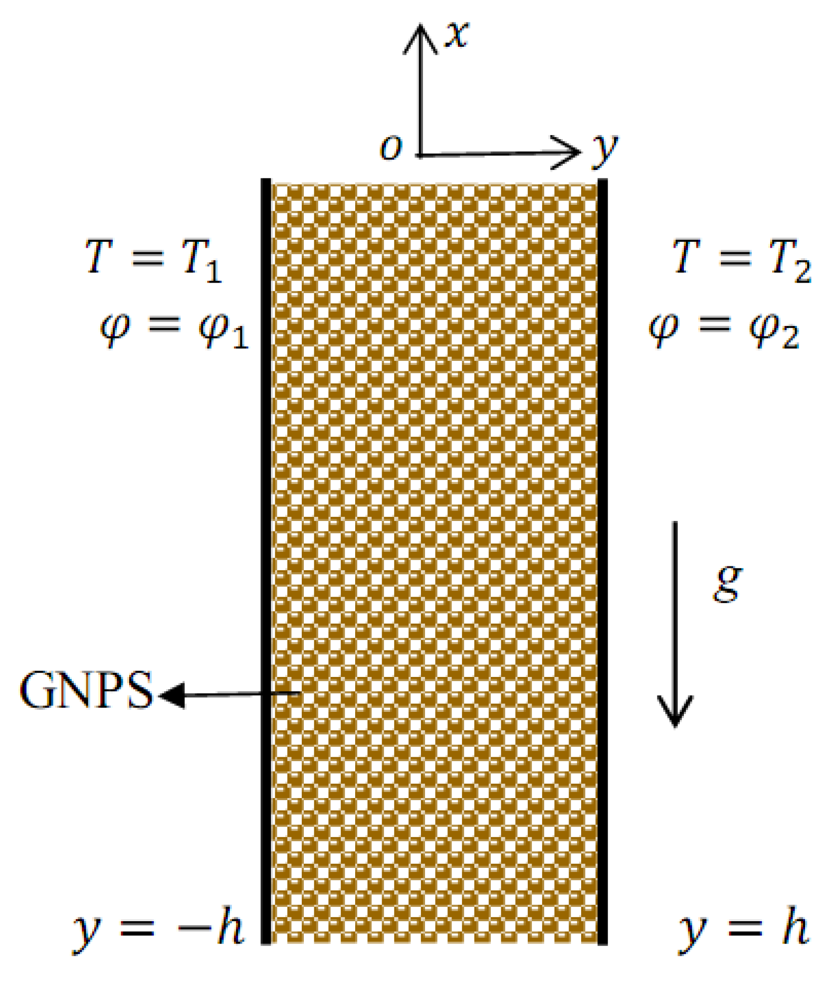
2. Mathematical Analysis

We considered the flow of the Jeffreys fluid with gold nanoparticles (GNPS) in a vertical layer and subjecting it to a transverse temperature gradient. We chose the coordinate system as in Figure 1. The vertical wall at $y=-h$ is prescribed at a uniform temperature $T_1$ and a uniform volumetric fraction of nanoparticles ${\phi }_1$, while the wall at $y=h$ is preserved at a uniform temperature $T_2 (>T_1)$ and a uniform volumetric fraction of nanoparticles ${\phi }_2 (>{\phi }_1)$. A Cartesian coordinate system $\left(x, y, z\right)$ is chosen with the origin at the middle of the fluid layer, the x$-$axis is vertical and oriented upward, y$-$axis is horizontal and perpendicular to the plates, while z$-$axis is horizontal, and the gravity $\overrightarrow{g}$ is acting in the negative $x-$direction.

According to the Oberbeck–Boussinesq approximation, i.e., the density variation is only experienced in the buoyancy term in the momentum equation. [18], the overall density of the nanofluid ρ is given by:

$$\rho =\phi {\rho }_p+\left(1-\phi \right)\left({\rho }_f-{\rho }_f{\beta }_T\left(T-T_1\right)\right)$$

where, ${\rho }_p$ is the particle density, ${\rho }_f$ is a reference density of the fluid, ${\beta }_T$ is the thermal volumetric expansion, φ is the nanoparticle.

The relevant basic equations under the Oberbeck–Boussinesq approximation are:

$$\nabla ·\overrightarrow{q}=0$$

(1)

$${\rho }_f\left[\frac{\partial \overrightarrow{q}}{\partial t}+\left(\overrightarrow{q}·\nabla \right)\overrightarrow{q}\right]=-\nabla p+\nabla ·{\tau }_{ij}-\left[\phi {\rho }_p+\left(1-\phi \right)\left({\rho }_f-{\rho }_f{\beta }_T\left(T-T_1\right)\right)\right]\overrightarrow{g}$$

(2)

$${\left(\rho c\right)}_f\left[\frac{\partial T}{\partial t}+\left(\overrightarrow{q}·\nabla \right)T\right]=k_T{\nabla }^{2}T+{\left(\rho c\right)}_P\left[D_B\left(\nabla \phi ·\nabla T\right)+\frac{D_T}{T_1}\left(\nabla T·\nabla T\right)\right]-\nabla q_r$$

(3)

$$\left[\frac{\partial \phi }{\partial t}+\left(\overrightarrow{q}·\nabla \right)\phi \right]=D_B{\nabla }^2\phi +\frac{D_T}{T_1}{k}_T{\nabla }^{2}T-k_o\left(\phi -{\phi }_1\right)$$

(4)

Physically, the dilute nanofluid suspension is considered and the temperature gradient is taken as a small quantity. Therefore, the term ${\beta }_T{\rho }_f\phi T$ can be excluded from Equation (2).

In the above equations, $\overrightarrow{q}=\left(u,v,w\right)$ is the velocity vector, ${\rho }_f$ is the fluid density, t is the time, $T$ is the temperature, $\phi$ is the nanoparticle volume fraction, ${\beta }_T$ is the fluid thermal volumetric expansion coefficient, ${\left(\rho c\right)}_f$ is the fluid heat capacity, ${\left(\rho c\right)}_p$ represent the heat capacity of the gold nanoparticles, $k_T$ is the thermal conductivity, $D_B$ is the Brownian diffusion coefficient, $D_T$ is the thermophoretic coefficient, $k_o$ is the chemical reaction parameter, $p$ is the pressure, and ${\tau }_{ij}$ the fluid stress tensor.

Using Rosseland’s approximation [13] for radiative heat flux $q_r$ we have:

$$q_r=-\frac{16{\sigma }^{*}{T}_m^3}{3k^{*}}\frac{\partial T}{\partial y}$$

(5)

where $T_m$, ${\sigma }^{*}$ and $k^{*}$ represent the mean temperature, Stefan–Boltzmann and Rosseland mean absorption coefficients.

Let us recall that the Jeffreys model uses the following rheological relation [22,23]:

$${\tau }_{ij}^{*}+{\lambda }_1^{*}\dot{{\tau }_{ij}^{*}}={\mu }^{*}\left[\dot{{\gamma }^{*}}+{\lambda }_2\ddot{{\gamma }^{*}}\right]$$

(6)

$\dot{{\gamma }^{*}}$ is the deformation tensor and $\ddot{{\gamma }^{*}}$ is the material derivative and these are given by:

$$\begin{array}{c}\dot{{\gamma }^{*}}=\nabla \overrightarrow{q}+{(\nabla \overrightarrow{q})}^T\\ \ddot{{\gamma }^{*}}=\frac{d\dot{{\gamma }^{*}}}{dt}=\frac{\partial \dot{{\gamma }^{*}}}{\partial t}+(\overrightarrow{q}\times \nabla )\dot{{\gamma }^{*}}\end{array}\begin{array}{c}{\displaystyle 〛}\end{array}$$

(7)

Putting Equation (6) into the Fourier transform domain yields:

$$({\tau }_{ij}+{\lambda }_1{\tau }_{ij})=\mu \left[\dot{\gamma }+{\lambda }_2\ddot{\gamma }\right]$$

(8)

where, ${\tau }_{ij}$ and $\dot{\gamma }$ are the Fourier transforms of the time histories of stress and rate of strain.

Here, $\mu$ is the viscosity, ${\lambda }_1$ is the ratio of relaxation to retardation time, ${\lambda }_2$ is the retardation time, $0<{\lambda }_2<{\lambda }_1$.

If ${\lambda }_1={\lambda }_2=0,$ then the problem characterizes the viscous fluid model.

If ${\lambda }_1\ne 0, {\lambda }_2=0,$ then the problem represents the second-grade fluid.

If ${\lambda }_1\ne 0, {\lambda }_2\ne 0,$ the problem signifies the Jeffreys fluid model.

Let us introduce the following dimensionless variables and quantities as:

$$x^{*}=\frac{x}{h},y^{*}=\frac{y}{h},q^{*}=\frac{qh}{{\alpha }_f},{\alpha }_f=\frac{k_T}{{\left(\rho c\right)}_f},t^{*}=\frac{t{\alpha }_f}{h^2},{\tau }_{ij}^{*}=\frac{{\tau }_{ij}{h}^2}{\mu {\alpha }_f},p^{*}=\frac{p{h}^2}{\mu {\alpha }_f},\theta =\frac{T-T_1}{T_2-T_1},{\phi }^{*}=\frac{\phi -{\phi }_1}{{\phi }_2-{\phi }_1}$$

(9)

After substituting from (6) and (7), Equations (1)–(4) can be written in dimensionless form after dropping the star mark as:

$$\nabla ·\overrightarrow{q}=0$$

(10)

$$\frac{1}{P_r}\left[\frac{\partial \overrightarrow{q}}{\partial t}+(\overrightarrow{q}·\nabla )\overrightarrow{q}\right]=-\nabla p+\frac{1}{1+{\lambda }_1}\nabla ·\left(1+\lambda \left(\frac{\partial \dot{\gamma }}{\partial t}+(\overrightarrow{q}\times \nabla )\right)\right)\dot{\gamma }-R_M+R_A\theta -R_N\phi$$

(11)

$$\frac{\partial \theta }{\partial t}+(\overrightarrow{q}·\nabla )\theta =(1+P_r{R}_n){\nabla }^2\theta +\frac{N_B}{L_e}(\nabla \phi ·\nabla \theta )+\frac{N_B{N}_A}{L_e}(\nabla \theta ·\nabla \theta )$$

(12)

$$\frac{\partial \phi }{\partial t}+(\overrightarrow{q}·\nabla )\phi =\frac{1}{L_e}{\nabla }^2\phi +\frac{N_A}{L_e}{\nabla }^2\theta -S\phi$$

(13)

The corresponding boundary conditions are:

$$\begin{gathered} \overrightarrow{q}=0 , \theta =0 , \phi =0 at y=-1 \\ \overrightarrow{q}=0 , \theta =1 , \phi =1 at y=1 \end{gathered}$$

(14)

The parameters are defined as:

$$\begin{array}{ll}{P}_r=\frac{\mu }{{\rho }_f{\alpha }_f},& R_M=\frac{\left({\rho }_p{\phi }_1+{\rho }_f(1-{\phi }_1)\right)g{h}^3}{\mu {\alpha }_f},R_A=\frac{g{\beta }_T{\rho }_f{h}^3(T_2-T_1)}{\mu {\alpha }_f},R_N=\frac{({\rho }_p-{\rho }_f)(1-{\phi }_1)g{h}^3}{\mu {\alpha }_f},\\ & R_n=\frac{16{\sigma }^{*}{T}_m^3}{3k^{*}\mu c_p},N_B=\frac{{(\rho c)}_P}{{(\rho c)}_f}({\phi }_2-{\phi }_1),N_A=\frac{D_T(T_2-T_1)}{D_B{T}_1({\phi }_2-{\phi }_1)},L_e=\frac{{\alpha }_f}{D_B},S=\frac{h^2{k}_o}{{\alpha }_f},\lambda =\frac{{\alpha }_f{\lambda }_2}{h^2}\end{array}$$

where $P_r$ is Prandtl number, $R_M$ is the basic density Rayleigh number, $R_A$ is the thermal Rayleigh number, $R_N$ is the concentration Rayleigh number, $R_n$ is the radiation parameter, $N_B$ is the modified particle density increment, $N_A$ is the modified diffusivity ratio, $L_e$ is the Lewis number, $S$ is the chemical reaction parameter, ${\alpha }_f$ is the thermal diffusivity of the fluid and $\lambda$ is the material parameter of the Jeffreys fluid.

2.1. Basic State

For the basic state, the flow is considered to be fully developed, unidirectional, steady and laminar. Thus, $\overrightarrow{q}={\overrightarrow{q}}_b=u_b\left(y\right)\widehat{i} , \theta ={\theta }_b\left(y\right), \phi ={\phi }_b\left(y\right), \frac{\partial p}{\partial x}=p_b$, where the subscript $b$ denotes the basic state. Under these circumstances, the governing equations reduced to:

$$0=-p_b+\frac{1}{1+{\lambda }_1}\frac{{\partial }^2{u}_b}{\partial y^2}-R_M+R_A{\theta }_b-R_N{\phi }_b$$

(15)

$$0=(1+P_r{R}_n)\frac{{\partial }^2{\theta }_b}{\partial y^2}+\frac{N_B}{L_e}\frac{\partial {\theta }_b}{\partial y}\frac{\partial {\phi }_b}{\partial y}+\frac{N_B{N}_A}{L_e}{(\frac{\partial {\theta }_b}{\partial y})}^2$$

(16)

$$0=\frac{1}{L_e}\frac{{\partial }^2{\phi }_b}{\partial y^2}+\frac{N_A}{L_e}\frac{{\partial }^2{\theta }_b}{\partial y^2}-S{\phi }_b$$

(17)

Solutions of basic state can be obtained and found to be:

$$\begin{gathered} u_b=\frac{1}{1440L_e\left(1+P_r{R}_n\right)}(\left(-1+y^2\right)\left(2S\left(3+y\right)\left(-25+3y\left(2+y\right)\right){L_e}^2\left(1+P_r{R}_n\right)R_N+120L_e\left(1+P_r{R}_n\right)\left(6p_b \\ -\left(3+y\right)R_A+6R_M+\left(3+y\right)R_N\right)+15\left(-5+y^2\right)\left(1+N_A\right)N_B\left(R_A+N_A{R}_N\right)\right)\left(1+{\lambda }_1\right)) \end{gathered}$$

(18)

$${\theta }_b=\frac{1}{8}\left(1+y\right)(4-\frac{\left(-1+y\right)\left(1+N_A\right)N_B}{L_e\left(1+P_r{R}_n\right)})$$

(19)

$${\phi }_b=\frac{1}{24}\left(1+y\right)(12+2S\left(-1+y\right)\left(3+y\right)L_e+\frac{3\left(-1+y\right)N_A\left(1+N_A\right)N_B}{L_e\left(1+P_r{R}_n\right)})$$

(20)

In the absence of the gold nanoparticles, the solution is in agreement with the plane Poiseuille flow where the velocity is given by:

$$u_b=\left(\frac{1+{\lambda }_1}{2}\right)(-h^2+y^2)p_b$$

2.2. Perturbed State and Linear Stability Analysis

For linear stability analysis, infinitesimal disturbances are imposed on the basic state in the following manner:

$$\overrightarrow{q}={\overrightarrow{q}}_b+{\overrightarrow{q}}^{\prime },\theta ={\theta }_b+{\theta }^{\prime },\phi ={\phi }_b+{\phi }^{\prime },p=p_b+p^{\prime },$$

(21)

where the primed quantities denote infinitesimal disturbance to the corresponding terms. Substituting from Equation (19) into Equations (8)–(11), we get:

$$\frac{\partial u^{\prime }}{\partial x}+\frac{\partial v^{\prime }}{\partial y}=0$$

(22)

$$\begin{gathered} \frac{1}{P_r}\left[\frac{\partial u^{\prime }}{\partial t}+u_b\frac{\partial u^{\prime }}{\partial x}+v^{\prime }\frac{\partial u_b}{\partial y}\right]=-\frac{\partial p^{\prime }}{\partial x}+\frac{1}{1+{\lambda }_1}\left(2\frac{{\partial }^2{u}^{\prime }}{\partial x^2}+\frac{{\partial }^2{u}^{\prime }}{\partial y^2}+\frac{{\partial }^2{v}^{\prime }}{\partial x\partial y}\right) \\ +\frac{\lambda }{1+{\lambda }_1}\left[2\frac{{\partial }^3{u}^{\prime }}{\partial t\partial x^2}+\frac{{\partial }^3{u}^{\prime }}{\partial t\partial y^2}+\frac{{\partial }^3{v}^{\prime }}{\partial t\partial x\partial y}\right]+R_A{\theta }^{\prime }-R_N{\phi }^{\prime } \end{gathered}$$

(23)

$$\frac{1}{P_r}\left[\frac{\partial v^{\prime }}{\partial t}+u_b\frac{\partial v^{\prime }}{\partial x}\right]=-\frac{\partial p^{\prime }}{\partial y}+\frac{1}{1+{\lambda }_1}\left(\frac{{\partial }^2{u}^{\prime }}{\partial x\partial y}+\frac{{\partial }^2{v}^{\prime }}{\partial x^2}+2\frac{{\partial }^2{v}^{\prime }}{\partial y^2}\right)+\frac{\lambda }{1+{\lambda }_1}\left[\frac{{\partial }^3{u}^{\prime }}{\partial t\partial x\partial y}+\frac{{\partial }^3{v}^{\prime }}{\partial t\partial x^2}+2\frac{{\partial }^3{v}^{\prime }}{\partial t\partial y^2}\right]$$

(24)

$$\frac{\partial {\theta }^{\prime }}{\partial t}+u_b\frac{\partial {\theta }^{\prime }}{\partial x}+v^{\prime }\frac{\partial {\theta }_b}{\partial y}=\left(1+P_r{R}_n\right)\left(\frac{{\partial }^2{\theta }^{\prime }}{\partial x^2}+\frac{{\partial }^2{\theta }^{\prime }}{\partial y^2}\right)+\frac{N_B}{L_e}\left(\frac{\partial {\theta }^{\prime }}{\partial y}-\frac{\partial {\phi }^{\prime }}{\partial y}\right)-2\frac{N_B{N}_A}{L_e}\frac{\partial {\theta }^{\prime }}{\partial y}$$

(25)

$$\frac{\partial {\phi }^{\prime }}{\partial t}+u_b\frac{\partial {\phi }^{\prime }}{\partial x}+v^{\prime }\frac{\partial {\phi }_b}{\partial y}=\frac{1}{L_e}\left(\frac{{\partial }^2{\phi }^{\prime }}{\partial x^2}+\frac{{\partial }^2{\phi }^{\prime }}{\partial y^2}\right)+\frac{N_A}{L_e}\left(\frac{{\partial }^2{\theta }^{\prime }}{\partial x^2}+\frac{{\partial }^2{\theta }^{\prime }}{\partial y^2}\right)-S{\phi }^{\prime }$$

(26)

We introduce a stream function $\psi \left(x,y,t\right)$ and the normal mode analysis, respectively, through:

$$u^{\prime }=\frac{\partial \psi }{\partial y},v^{\prime }=-\frac{\partial \psi }{\partial x}$$

(27)

$$\left(\psi ,{\theta }^{\prime },{\phi }^{\prime }\right)=\left(\mathsf{\Psi },\mathsf{\Theta },\mathsf{\Phi }\right)\left(y\right)e^{ia\left(x-ct\right)}$$

(28)

where a is the vertical wavenumber and $c=c_r+i{c}_i$ is the complex wave speed. The sign of $c_i$ determines the growth or decay of the disturbances, i.e., accordingly, the flow is linearly stable, neutrally stable, or unstable as, $c_i=0$ or $c_i>0$. Equations (27) and (28) are substituted back into Equations (22)–(26) and the pressure is eliminated from the momentum equation and adopts the shorthand notation $\frac{d}{dy}$ so that we are led to linearized stability equations, namely:

$$\frac{ia}{P_r}\left[\left(u_b-c\right)\left(D^2-a^2\right)-D^2{u}_b\right]\mathsf{\Psi }=\frac{1}{1+{\lambda }_1}\left(1-iac\lambda \right){\left(D^2-a^2\right)}^2\mathsf{\Psi }+R_{A}D\mathsf{\Theta }-R_{N}D\mathsf{\Phi }$$

(29)

$$ia\left[\left(u_b-c\right)\mathsf{\Theta }-D{\theta }_b\mathsf{\Psi }\right]=(1+P_r{R}_n)(D^2-a^2)\mathsf{\Theta }+\frac{N_B}{L_e}D(\mathsf{\Theta }-\mathsf{\Phi })-\frac{2N_B{N}_A}{L_e}D\mathsf{\Theta }$$

(30)

$$ia\left[\left(u_b-c\right)\mathsf{\Phi }-D{\varphi }_b\mathsf{\Psi }\right]=\frac{1}{L_e}(D^2-a^2)\mathsf{\Phi }+\frac{N_A}{L_e}(D^2-a^2)\mathsf{\Theta }-S\mathsf{\Phi }$$

(31)

The boundary conditions now become:

$$\mathsf{\Psi }=D\mathsf{\Psi }=\mathsf{\Theta }=\mathsf{\Phi }=0 \mathrm{at} y=\pm 1$$

(32)

3. Numerical Procedure

Equations (29)–(31) with the boundary conditions (32) constitute an eigenvalue problem. This can be solved numerically by using the Chebyshev collocation method. The kth order Chebyshev polynomial is given by:

$${\xi }_k\left(y\right)=cosk\theta ,\theta ={cos}^{-1}y$$

(33)

The Chebyshev collocation points are given by:

$$y_j=cos\left(\frac{\pi j}{N}\right),j=0\left(1\right)N$$

(34)

Here, the right and left wall boundaries correspond to $j=0$ and $N$, respectively. The field variable $\mathsf{\Psi }, \mathsf{\Theta }$ and $\mathsf{\Phi }$ can be approximated in terms of the Chebyshev variable as follows:

$$\mathsf{\Psi }\left(y\right)={\displaystyle \sum }_{j=0}^N{\xi }_n\left(y_j\right){\mathsf{\Psi }}_j,\mathsf{\Theta }\left(y\right)={\displaystyle \sum }_{j=0}^N{\xi }_n\left(y_j\right){\mathsf{\Theta }}_j,\mathsf{\Phi }\left(y\right)={\displaystyle \sum }_{j=0}^N{\xi }_n\left(y_j\right){\mathsf{\Phi }}_j$$

(35)

where ${\mathsf{\Psi }}_j$, ${\mathsf{\Theta }}_j$ and ${\mathsf{\Phi }}_j$ are constant. Equations (27)–(30) are discretized in Chebyshev polynomials to get:

$$\begin{gathered} \frac{ia}{P_r}\left[\left(u_b-c\right)\left({\displaystyle \sum }_{k=0}^N{B}_{jk}{\mathsf{\Psi }}_k-a^2{\mathsf{\Psi }}_j\right)-D^2{u}_b{\mathsf{\Psi }}_j\right] \\ =\frac{1}{1+{\lambda }_1}(1-iac\lambda )\left({\displaystyle \sum }_{k=0}^N{C}_{jk}{\mathsf{\Psi }}_k-2a^2{\displaystyle \sum }_{k=0}^N{B}_{jk}{\mathsf{\Psi }}_k+a^4{\mathsf{\Psi }}_j\right) \\ +R_A{\displaystyle \sum }_{k=0}^N{A}_{jk}{\mathsf{\Theta }}_k-R_N{\displaystyle \sum }_{k=0}^N{A}_{jk}{\mathsf{\Phi }}_k,j=1\left(1\right)N-1 \end{gathered}$$

(36)

$$\begin{gathered} ia\left[\left(u_b-c\right){\mathsf{\Theta }}_j-D{\theta }_b{\mathsf{\Psi }}_j\right]=\left(1+P_r{R}_n\right)\left({\displaystyle \sum }_{k=0}^N{B}_{jk}{\mathsf{\Theta }}_k-a^2{\mathsf{\Theta }}_j\right)+\frac{N_B}{L_e}\left[{\displaystyle \sum }_{k=0}^N{A}_{jk}{\mathsf{\Theta }}_k-{\displaystyle \sum }_{k=0}^N{A}_{jk}{\mathsf{\Phi }}_k\right] \\ -\frac{2N_B{N}_A}{L_e}{\displaystyle \sum }_{k=0}^N{A}_{jk}{\mathsf{\Theta }}_k,j=1\left(1\right)N-1 \end{gathered}$$

(37)

$$ia\left[\left(u_b-c\right){\mathsf{\Phi }}_j-D{\varphi }_b{\mathsf{\Psi }}_j\right]=\frac{1}{L_e}\left({\displaystyle \sum }_{k=0}^N{B}_{jk}{\mathsf{\Phi }}_k-a^2{\mathsf{\Phi }}_j\right)+\frac{N_B}{L_e}\left({\displaystyle \sum }_{k=0}^N{B}_{jk}{\mathsf{\Theta }}_k-a^2{\mathsf{\Theta }}_j\right)-S{\mathsf{\Phi }}_j,j=1\left(1\right)N-1$$

(38)

$${\mathsf{\Psi }}_0={\mathsf{\Psi }}_N=0$$

(39)

$${\displaystyle \sum }_{k=0}^N{A}_{jk}{\mathsf{\Psi }}_k=0,j=0\&N$$

(40)

$${\mathsf{\Theta }}_0={\mathsf{\Theta }}_N=0$$

(41)

$${\mathsf{\Phi }}_0={\mathsf{\Phi }}_N=0$$

(42)

where

$$A_{jk}=\{\begin{array}{l}\frac{c_j{\left(-1\right)}^{k+j}}{c_k\left(y_j-y_k\right)}j\ne k\\ \frac{y_j}{2\left(1-y_j^2\right)}1\le j=k\le N-1\\ \frac{2N^2+1}{6}j=k=0\\ -\frac{2N^2+1}{6}j=k=N\end{array}$$

(43)

$$B_{jk}=A_{jm}·A_{mk} \mathrm{and} C_{jk}=B_{jm}·B_{mk}$$

(44)

with

$$c_j=\{\begin{array}{l}2 j=0,N\\ 1 1\le j\le N-1\end{array}$$

The above equations form the following system of linear algebraic equations:

$$AX=cBX$$

(45)

where $A$ and $B$ are the square complex matrices of order $3\left(N+1\right)$, $c$ is the complex eigenvalue and $X$ is the eigenfunction. The above generalized eigenvalue problem usually describes the linear stability boundary of the basic flow, based on the QZ algorithm (Moler and Stewart [24]), the eigenvalues of the eigenvalue problem are calculated with a home-made computational code which was written in Mathematica 11.3 (© Wolfram Research) software [18,24].

4. Results and Discussion

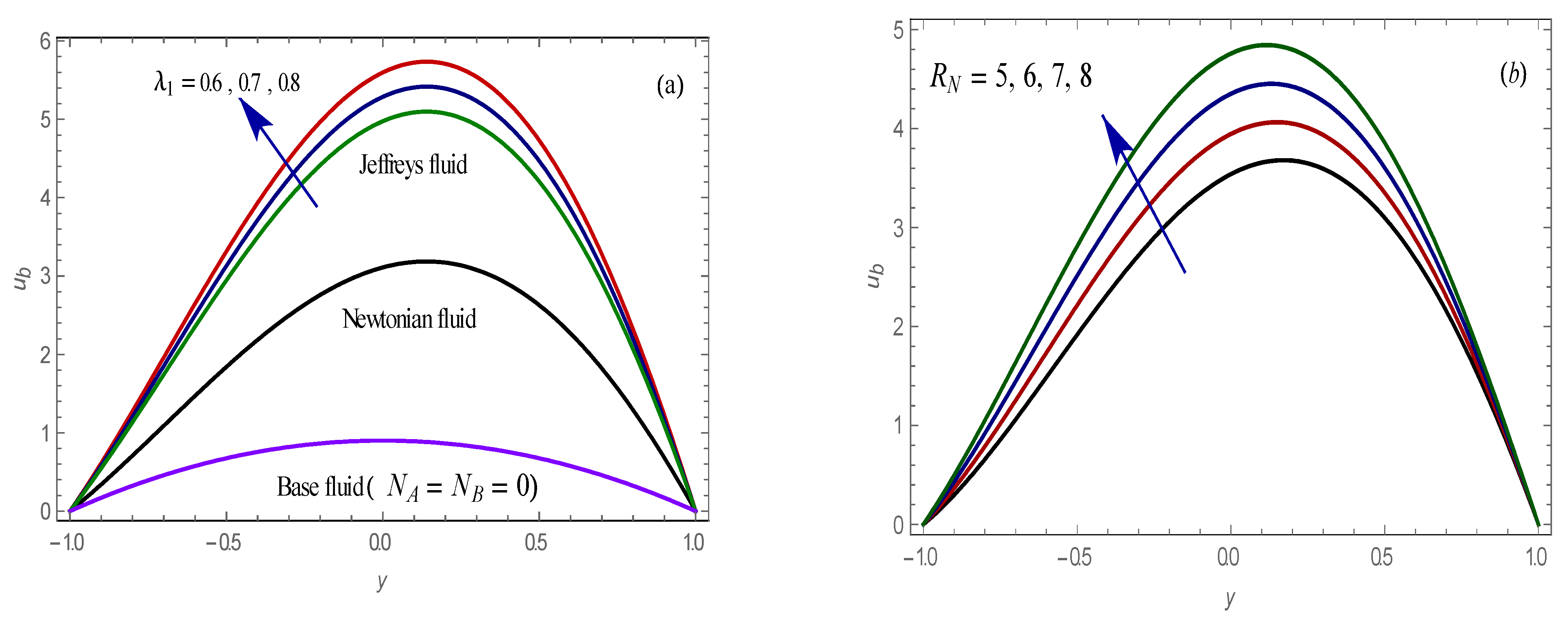
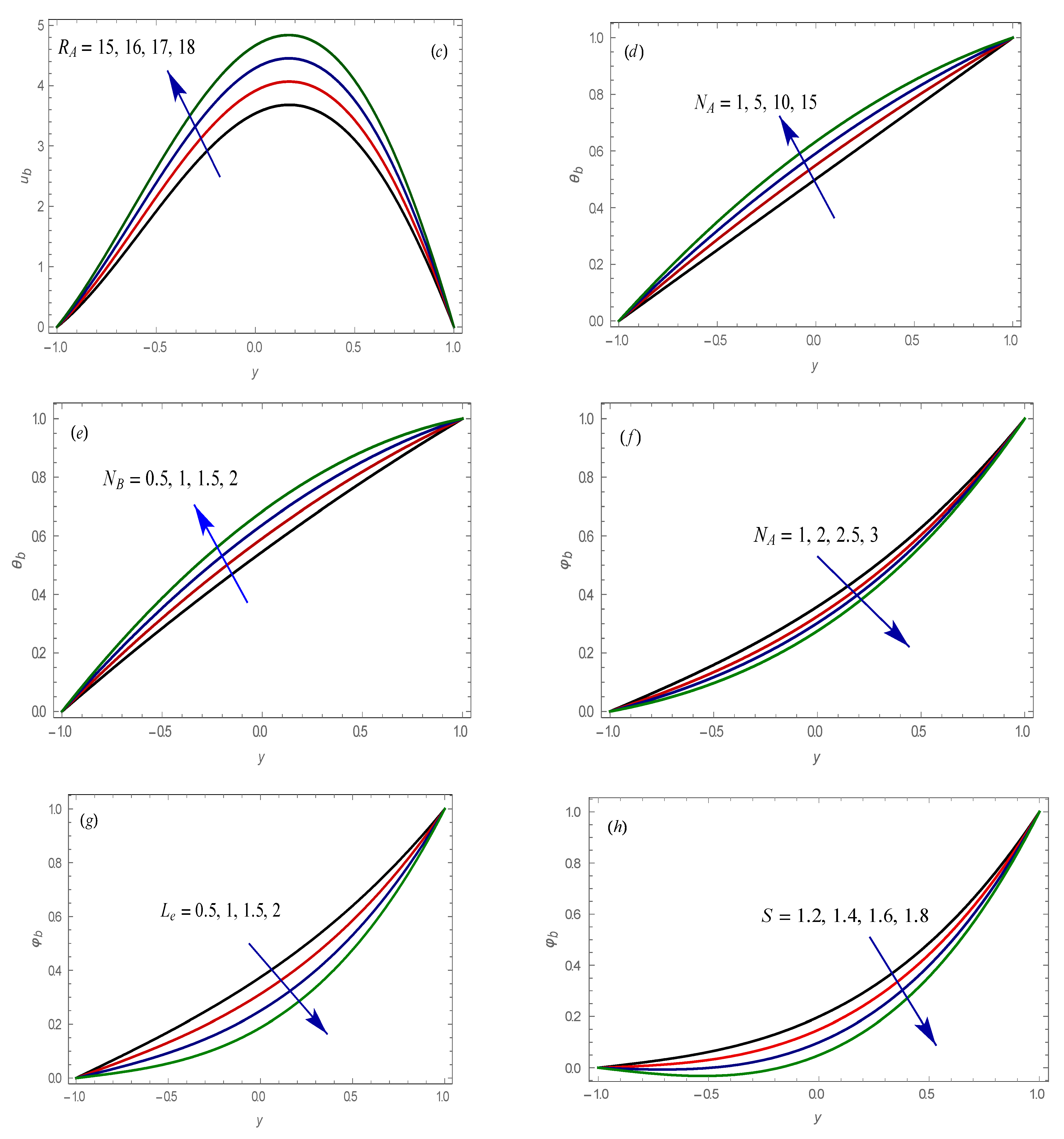
4.1. Base Flow

In this piece of our examination, we have graphically portrayed the effects of different actual parameters on base velocity $u_b$, temperature ${\theta }_b$, and nanoparticles fixation ${\varnothing }_b$ on account of their fundamental state. The impact was displayed graphically in Figure 2a–h.

The impact of basic state parameters on the velocity curves of the flow are delineated in Figure 2a–c for different values of the ratio of relaxation to retardation time ${\lambda }_1$ (Figure 2a), concentration Rayleigh number $R_N$ (Figure 2b) and thermal Rayleigh number $R_A$ (Figure 2c). Figure 2a illustrate a comparison between the velocity for the base fluid, Newtonian fluid and Jeffreys fluid which show that the velocity is higher in the case of the Jeffreys fluid. Additionally, it is observed from Figure 2b,c that the velocity increased by increasing the concentration Rayleigh number and thermal Rayleigh number. Figure 2d,e are outlined to examine the impacts of the modified diffusivity ratio $N_A$ (Figure 2d) and modified particle density increment $N_B$ (Figure 2e) on the temperature for the Jeffreys fluid with nanoparticles. From this plot, we identified that the expansion in the values of $N_A$, and $N_B$ amplifies the temperature. This is reliable with the physicality’s concerned as the modified particle density increment depends on the unsystematic motion of fluid particles on the surface and the rise of $N_B$ enhance this motion of the fluid particles which causes more of heat. Likewise, the expanding values of $N_A$ physically implies that the nanoparticles are moving far from the hot surface to cool which causes a fluid temperature rise. Figure 2f–h are intended to research the effects of the modified diffusivity ratio $N_A$ (Figure 2f), Lewis number $L_e$ (Figure 2g), and chemical reaction parameter $S$ (Figure 2h). It can be seen from these plots that the concentration of the nanoparticles decay with the expansion of $N_A$, $L_e$, and $S$.

4.2. Validation of the Code

We checked the accuracy and validity of our numerical code by varying the order of the Chebyshev polynomials (i.e., the number of collocation points) along with different sets of parameters. It is shown from

Table 1. The effect of the various governing parameters on the critical thermal Rayleigh number $R_{Ac}$, the critical wavenumber $a_c$ and the critical wave speed $c_c$ obtained by the numerical solution of Equations (29)–(32). $N$ is the number of terms in the expansions (35) for $R_{Ac}$, $a_c$ and $c_c$ to converg.

N	Le = 0.5, Pr = 0.7, λ1 = 0.6, RN = 100, Rn = 1, pb = 1, S = 1.2, RM = 100, NA = 1, NB = 0.5, λ = 0.2			N	Le = 2, Pr = 0.7, λ1 = 0.6, RN = 100, Rn = 1, pb = 1, S = 1.2, RM = 100, NA = 1, NB = 0.5, λ = 0.2			N	Le = 0.5, Pr = 1, λ1 = 0.6, RN = 100, Rn = 1, pb = 1, S = 1.2, RM = 100, NA = 1, NB = 0.5, λ = 0.2
	ac	RAc	cc		ac	RAc	cc		ac	RAc	cc
5	1.3926	307.6482	14.6398	5	1.4268	270.8822	10.0793	5	1.2421	407.6655	21.5326
10	0.8509	523.6534	43.4964	10	0.9427	450.7811	31.1460	10	0.6363	951.5356	77.2332
15	0.8560	518.1818	42.7893	15	0.9459	447.8552	30.8200	15	0.6406	939.3423	76.0186
20	0.8560	518.1818	42.7893	20	0.9459	447.8554	30.8200	20	0.6406	939.3429	76.0186
N	Le = 0.5, Pr = 0.7, λ1 = 0.9, RN = 100, Rn = 1, pb = 1, S = 1.2, RM = 100, NA = 1, NB = 0.5, λ = 0.2			N	Le = 0.5, Pr = 0.7, λ1 = 0.6, RN = 500, Rn = 1, pb = 1,S = 1.2, RM = 100, NA = 1, NB = 0.5, λ = 0.2			N	Le = 0.5, Pr = 0.7, λ1 = 0.6, RN = 100, Rn = 10, pb = 1, S = 1.2, RM = 100, NA = 1, NB = 0.5, λ = 0.2
	ac	RAc	cc		ac	RAc	cc		ac	RAc	cc
5	1.4921	243.9072	6.9705	5				5	1.3611	310.9509	6.2310
10	1.1481	314.4263	19.9220	10	0.7326	964.5307	78.7104	10	1.0310	452.4231	23.0459
15	1.1503	313.5978	19.7783	15	0.7398	952.9166	77.2331	15	1.0310	452.1279	23.0146
20	1.1503	313.5976	19.7783	20	0.7398	952.9190	77.2334	20	1.0310	452.1278	23.0146
25	1.1503	313.5976	19.7783	25	0.7398	952.9190	77.2334	25	1.0310	452.1278	23.0146
N	Le = 0.5, Pr = 0.7, λ1 = 0.6, RN = 100, Rn = 1, pb = 10, S = 1.2, RM = 100, NA = 1, NB = 0.5, λ = 0.2			N	Le = 0.5, Pr = 0.7, λ1 = 0.6, RN = 100, Rn = 1, pb = 1, S = 1.8, RM = 100, NA = 1, NB = 0.5, λ = 0.2			N	Le = 0.5, Pr = 0.7, λ1 = 0.6, RN = 100, Rn = 1, pb = 1, S = 1.2, RM = 1000, NA = 1, NB = 0.5, λ = 0.2
	ac	RAc	cc		ac	RAc	cc		ac	RAc	cc
5	1.4068	304.3978	12.0650	5	1.3983	304.2107	15.5356	5	1.2541	321.5724	−191.9384
10	0.8841	504.0515	38.9607	10	0.8459	522.6236	44.6216	10	0.5626	866.0277	−107.9221
15	0.8892	499.2325	38.3358	15	0.8512	516.8656	43.8780	15	0.5620	860.8959	−108.6310
20	0.8892	499.2324	38.3357	20	0.8512	516.8657	43.8780	20	0.5620	860.8961	−108.6310
25	0.8892	499.2324	38.3357	25	0.8512	516.8657	43.8780	25	0.5620	860.8961	−108.6310
N	Le = 0.5, Pr = 0.7, λ1 = 0.6, RN = 100, Rn = 1, pb = 1, S = 1.2, RM = 100, NA = 4, NB = 0.5, λ = 0.2			N	Le = 0.5, Pr = 0.7, λ1 = 0.6, RN = 100, Rn = 1, pb = 1, S = 1.2, RM = 100, NA = 1, NB = 2, λ = 0.2			N	Le = 0.5, Pr = 0.7, λ1 = 0.6, RN = 100, Rn = 1, pb = 1, S = 1.2, RM = 100, NA = 1, NB = 0.5, λ = 0.5
	ac	RAc	cc		ac	RAc	cc		ac	RAc	cc
5	1.4197	319.2867	54.0587	5	1.4211	314.4287	49.6449	5	1.1724	313.0687	8.2348
10	0.6824	624.9957	102.1356	10	0.6690	631.3779	111.7336	10	0.4296	1115.9144	64.6064
15	0.6910	610.2450	99.7242	15	0.6788	615.2087	108.4975	15	0.4349	1091.6271	62.9311
20	0.6910	610.2486	99.7248	20	0.6788	615.2125	108.4983	20	0.4349	1091.6281	62.9311
25	0.6910	610.2486	99.7248	25	0.6788	615.2125	108.4983	25	0.4349	1091.6281	62.9311

that N = 30 collocation points are usually sufficient to find the critical thermal Rayleigh number $R_{Ac}$, the corresponding critical wave number $a_c$, and the critical wave speed $c_c$ (four decimal point accuracy) by linear stability theory. Hence, the results are obtained by taking N = 30 in all further computations.

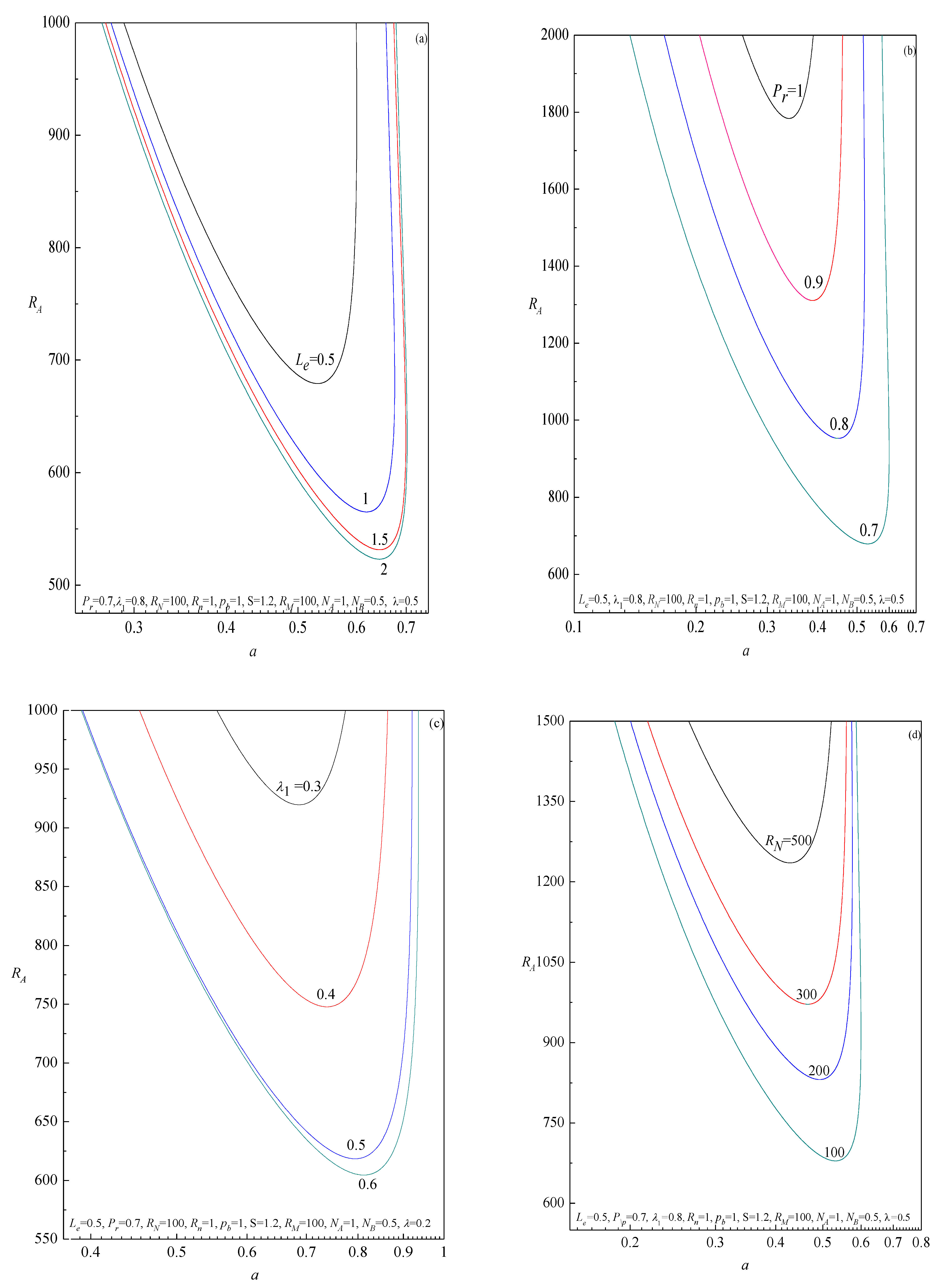
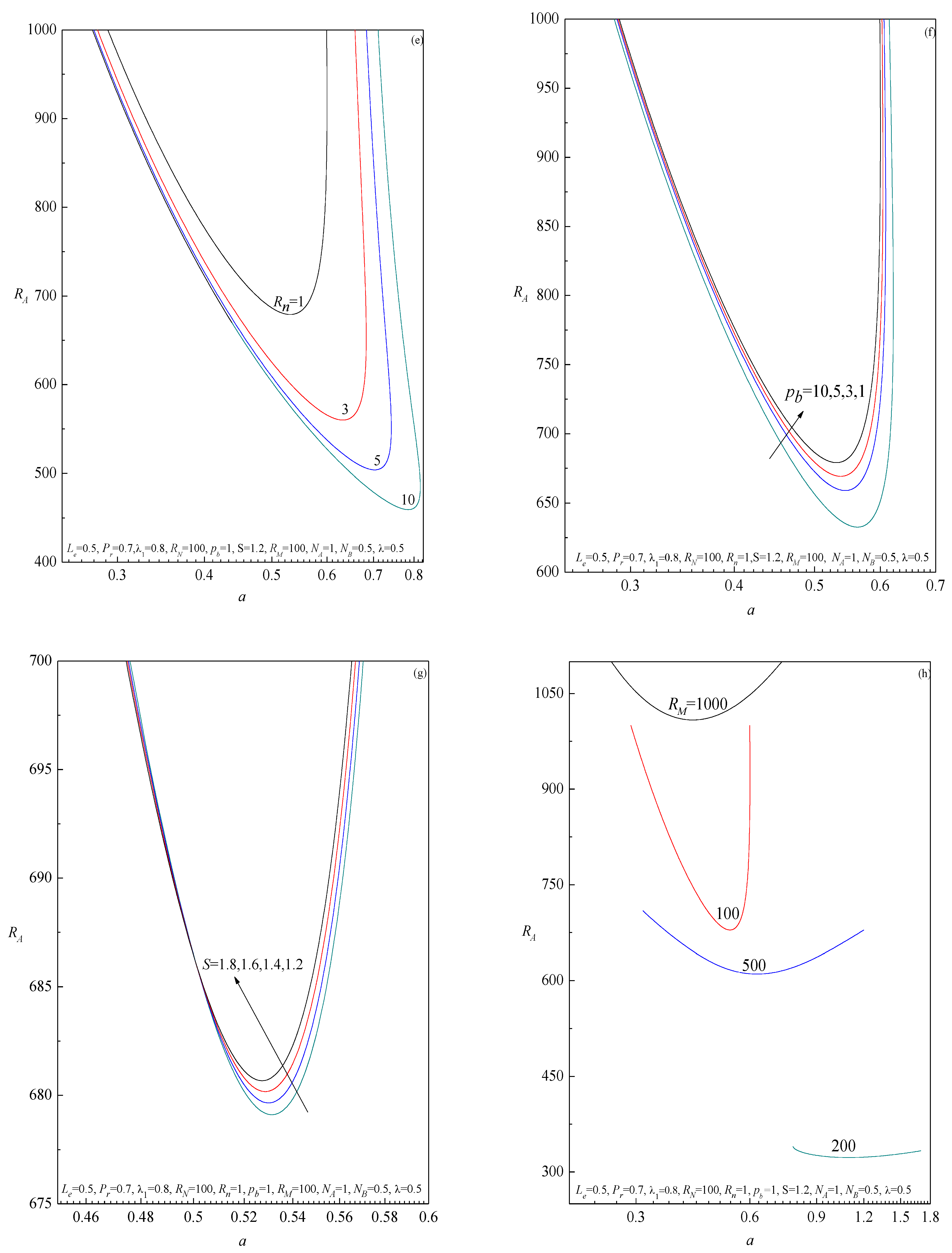
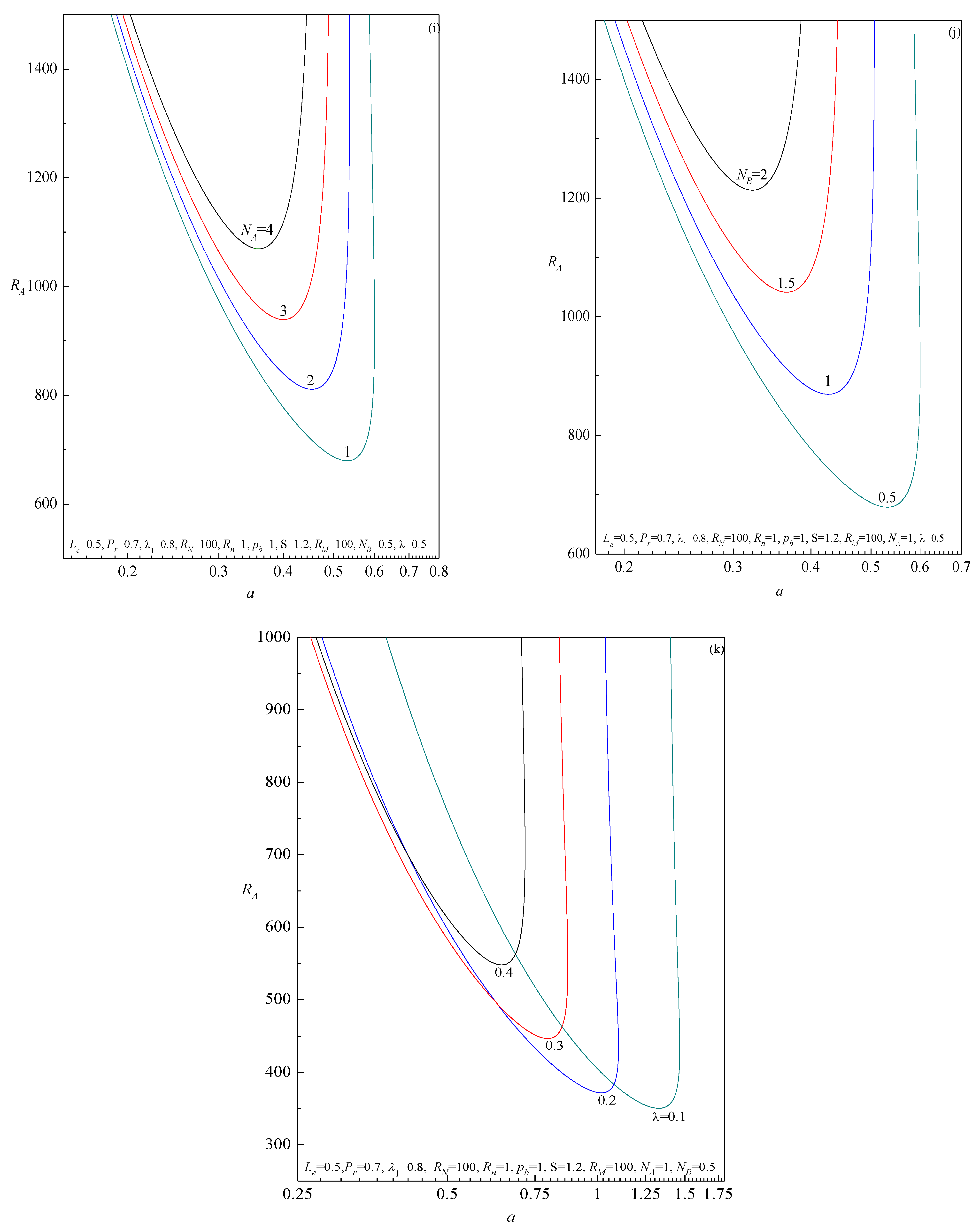
4.3. Neutral Stability Curves

The curve of neutral stability is obtained by prescribing a vanishing growth rate of the perturbation modes, $c_i=0$. These curves, plotted for a fixed controlling parameter in the ($a, R_A$)–plane, represent the threshold between linear stability and instability. The instability region $\left(c_i>0\right)$ is enclosed by the neutral stability curve, while the stability region is below and outside the curve. As a consequence, the absolute minimum of the neutral stability curve yields the so-called critical value of $a,{ R}_A$, and $c$ which are denoted by $a_c,R_{AC}$ and $c_c$, respectively. The physical meaning of the critical conditions is that no linear instability is possible for $R_A<R_{Ac}$. The neutral stability curves are displayed in Figure 3a–k for different values of the Lewis number $L_e$ (Figure 3a), Prandtl number $P_r$ (Figure 3b), the ratio of relaxation to retardation time ${\lambda }_1$ (Figure 3c), concentration Rayleigh number $R_N$ (Figure 3d), radiation parameter $R_n$ (Figure 3e), pressure gradient $p_b$ (Figure 3f), chemical reaction parameter $S$ (Figure 3g), basic density Rayleigh number $R_M$ (Figure 3h), modified diffusivity ratio $N_A$ (Figure 3i), modified particle density increment $N_B$ (Figure 3j) and material parameter of the Jeffreys fluid $\lambda$ (Figure 3k). It is observed from the figures that the instability always sets in via traveling-wave mode $\left(c_c\ne 0\right)$, irrespective of the values of the control parameters. From these figures, it follows that an increase in the value of $L_e, {\lambda }_1, R_n, p_b$ and, $S$ is to decrease the minimum of the thermal Rayleigh number indicating that their effect is to decrease the region of stability. Whereas, increasing $P_r$, $R_N,$ $N_A, N_B$ and $\lambda$ enhances the stability of the basic flow. The Brownian motion effect appears only through the Lewis number. The increasing of the Lewis number destabilizes the fluid flow. Interestingly, the effect of increasing $R_M$ shows a mixed behavior on the stability characteristics of the system. We also demonstrated that the critical thermal Rayleigh number shifts towards smaller values of the wavenumber $a$ with increasing $P_r$, $R_N,$ $N_A, N_B$ and $\lambda$ indicating that the cell width increases, while an opposite trend is observed with increasing $L_e,{\lambda }_1,R_n,p_b$ and, $S$ and $a_c$ shows two-fold behavior with increasing $R_M$.

The similarities and differences between the Newtonian fluid (NF) (${\lambda }_1=\lambda =0$), second-grade fluid (SF) (${\lambda }_1=0.5,\lambda =0$) and the Jeffreys fluid (JF) (${\lambda }_1=0.5,\lambda =0.2$) models in the presence of gold nanoparticles are tabulated in Table 1 and

Table 2. Comparison between the critical stability parameters of the Newtonian, second-grade and Jeffreys fluids for various governing parameters.

${\mathit{L}}_{\mathit{e}}$	${\mathit{P}}_{\mathit{r}}$	${\mathit{R}}_{\mathit{N}}$	${\mathit{R}}_{\mathit{n}}$	${\mathit{p}}_{\mathit{b}}$	$\mathit{S}$	${\mathit{R}}_{\mathit{M}}$	${\mathit{N}}_{\mathit{A}}$	${\mathit{N}}_{\mathit{B}}$	Newtonian Fluid $({\mathit{\lambda }}_1=\mathit{\lambda }=0)$			Second-Grade Fluid $({\mathit{\lambda }}_1=0.5$, $\mathit{\lambda }=0)$			Jeffreys Fluid $({\mathit{\lambda }}_1=0.5$, $\mathit{\lambda }=0.2)$
									${\mathit{a}}_{\mathit{c}}$	${\mathit{R}}_{\mathit{A}\mathit{c}}$	${\mathit{c}}_{\mathit{c}}$	${\mathit{a}}_{\mathit{c}}$	${\mathit{R}}_{\mathit{A}\mathit{c}}$	${\mathit{c}}_{\mathit{c}}$	${\mathit{a}}_{\mathit{c}}$	${\mathit{R}}_{\mathit{A}\mathit{c}}$	${\mathit{c}}_{\mathit{c}}$
0.5	0.7	100	1	1	1.2	100	1	0.5	0.9940	10,392.65	864.5781	0.9951	4642.71	567.1697	0.7941	618.43	50.7498
1									0.9573	14,132.58	1013.3955	0.9574	6323.88	668.7228	0.8515	571.93	39.9794
2									0.9356	16,907.73	1116.3420	0.9361	7509.17	735.4287	0.8669	545.40	38.0532
	0.8								0.9903	12,242.60	1004.9593	0.9910	5473.60	661.5412	0.7147	768.49	62.3736
	1								0.9839	16,135.24	1293.1352	0.9840	7220.91	855.1587	0.5998	1140.61	86.9350
		200							0.9958	10,327.92	857.7339	0.9994	4575.61	556.5940	0.7624	732.89	59.1921
		500							1.0016	10,129.66	836.8116	1.0136	4363.20	523.3194	0.7051	1051.41	81.5126
			5						0.9460	15,471.22	1062.3798	0.9459	6956.57	703.5628	0.8945	557.05	34.2217
			10						0.9308	17,573.54	1138.3208	0.9300	7933.93	757.1569	0.9252	547.32	30.7248
				5					0.9940	10,397.03	864.4272	0.9950	4646.95	566.9162	0.8037	610.80	49.0667
				10					0.9940	10,402.49	864.2481	0.9950	4652.24	566.6301	0.8167	600.86	46.9125
					1.4				0.9941	10,383.78	864.2200	0.9954	4633.65	566.6079	0.7930	617.82	51.0560
					1.8				0.9943	10,366.04	863.5012	0.9958	4615.51	565.4802	0.7910	616.59	51.6657
						500			0.9916	10,816.78	848.7251	0.9903	5027.08	539.2726	0.8512	606.53	−31.9050
						1000			0.9889	11,299.04	825.7010	0.9898	5285.42	481.5624	0.5889	915.59	−91.8284
							2		1.0242	8002.73	760.9271	1.0286	3507.08	491.9218	0.7345	660.37	67.5225
							4		1.0717	5191.24	625.8271	1.0863	2112.73	387.4967	0.6563	717.14	106.3018
								1	1.0469	6534.64	692.7507	1.0517	2870.97	446.3826	0.7163	672.46	74.3268
								2	1.1094	3549.30	536.7460	1.1218	1505.72	334.9832	0.6405	726.35	118.5282

. The instability characteristics of the system analyzed for the same parametric values for all the three fluids are qualitatively different. It is observed that $R_{Ac}{}^{\left(NF\right)}>R_{Ac}{}^{\left(SF\right)}>R_{Ac}{}^{\left(JF\right)}$ irrespective of values of the governing parameters, i.e., the Newtonian fluid has a more stabilizing effect than other fluids while the Jeffreys fluid is the least stable. The size of the convection cell for the Jeffreys fluid is more, compared to other fluids. The table also shows that travelling-wave convection is found to be a preferred mode of instability for all the fluids.

5. Concluding Remarks

This paper examined the stability analysis of the Jeffreys fluid model with gold nanoparticles under the effect of radiation and chemical reaction in a vertical fluid layer. The dimensionless parameters driving the instability are the thermal Rayleigh number $R_A$, Lewis number $L_e$, Prandtl number $P_r$, the ratio of relaxation to retardation time ${\lambda }_1$, concentration Rayleigh number $R_N$, radiation parameter $R_n$, chemical reaction parameter $S$, basic density Rayleigh number $R_M$, modified diffusivity ratio $N_A$ and modified particle density increment $N_B$. A modal linear stability analysis of small-amplitude disturbances was performed, leading to the formulation of the stability eigenvalue problem which has been solved numerically by employing the Chebyshev collocation method. The investigations bring out interesting features of the basic field and stability characteristics of the basic state. The main results of our study can be epitomized in the following points:

• The influences of the basic state parameters on the velocity, temperature and nanoparticles concentration were exhibited graphically.
• The preferred mode of instability is traveling-wave mode irrespective of the values of governing parameters.
• The effect of increasing $L_e, {\lambda }_1, R_n, p_b$ and, $S$ is to hasten the onset of instability.
• The presence of $P_r, R_N, N_A, N_B$ and $\lambda$ is to reinforce stability of the system. The density Rayleigh number instills both stabilizing and destabilizing effects on the basic flow.
• Newtonian fluid has a more stabilizing effect than second-grade and the Jeffreys fluids in the presence of gold nanoparticles; the Jeffreys fluid being the least stable.

References

1. Hussain, F.; Ellahi, R.; Zeeshan, A.; Vafai, K. Modelling study on heated couple stress fluid peristaltically conveying gold nanoparticles through coaxial tubes: A remedy for gland tumors and arthritis. J. Mol. Liq. 2018, 268, 149–155. [Google Scholar] [CrossRef]
2. Mekheimer, K.S.; Hasona, W.M.; Abo-Elkhair, R.E.; Zaher, A.Z. Peristaltic blood flow with gold nanoparticles as a third grade nanofluid in catheter: Application of cancer therapy. Phys. Lett. A 2018, 382, 85–93. [Google Scholar] [CrossRef]
3. Ebaid, A.; Aljohani, A.F. Homotopy perturbation method for peristaltic motion of gold-blood nanofluid with heat source. Int. J. Numer. Methods Heat Fluid Flow 2020, 30, 3121–3138. [Google Scholar] [CrossRef]
4. Abd Elmaboud, Y.; Mekheimer, K.S.; Emam, T.G. Numerical examination of gold nanoparticles as a drug carrier on peristaltic blood flow through physiological vessels: Cancer therapy treatment. BioNanoScience 2019, 9, 952–965. [Google Scholar] [CrossRef]
5. Eldabe, N.T.; Ramadan, S.F. Impacts of peristaltic flow of micropolar fluid with nanoparticles through a porous medium under the effects of heat absorption and wall properties: Homotopy perturbation method. Heat Transf. 2020, 49, 889–908. [Google Scholar] [CrossRef]
6. Eldabe, N.; Ramadan, S.; Awad, A. Analytical and numerical treatment to study the effects of hall currents with viscous dissipation, heat absorpation and chemical reaction on peristaltic flow of Carreau nanofluid. Therm. Sci. 2021, 25, 181–196. [Google Scholar] [CrossRef]
7. Eldabe, N.T.; Kamel, K.A.; Ramadan, S.F.; Saad, R.A. Peristaltic motion of Eyring-Powell nano fluid with couple stresses and heat and mass transfer through a porous media under the effect of magnetic field inside asymmetric vertical channel. J. Adv. Res. Fluid Mech. Therm. Sci. 2020, 68, 58–71. [Google Scholar] [CrossRef]
8. Orszag, S.A. Accurate solution of the Orr–Sommerfeld stability equation. J. Fluid Mech. 1971, 50, 689–703. [Google Scholar] [CrossRef] [Green Version]
9. Drazin, P.G. Introduction to Hydrodynamic Stability; Cambridge University Press (CUP): Cambridge, UK, 2002; p. 32. [Google Scholar]
10. Makinde, O.D. Chebyshev collocation approach to stability of blood flows in a large artery. Afr. J. Biotechnol. 2012, 11, 9881–9887. [Google Scholar] [CrossRef]
11. Chimetta, B.P.; de Moraes Franklin, E. Asymptotic and Numerical Solutions of the Orr-Sommerfeld Equation for a Thin Liquid Film on an Inclined Plane. In Proceedings of the IV Journeys in Multiphase Flows (JEM2017), São Paulo, Brazil, 27–31 March 2017. [Google Scholar]
12. Lin, J.; Xia, Y.; Bao, F. Hydrodynamic instability of nanofluids in a channel flow. Fluid Dyn. Res. 2014, 46, 055512. [Google Scholar] [CrossRef]
13. Xia, Y.; Lin, J.; Bao, F.; Chan, T.L. Flow instability of nanofluids in jet. Appl. Math. Mech. 2015, 36, 141–152. [Google Scholar] [CrossRef]
14. Anuar, N.S.; Bachok, N.; Arifin, N.M.; Rosali, H. MHD flow past a nonlinear stretching/shrinking sheet in carbon nanotubes: Stability analysis. Chin. J. Phys. 2020, 65, 436–446. [Google Scholar] [CrossRef]
15. Hussain, Z.; Rehman, A.U.; Zeeshan, R.; Sultan, F.; Hamid, T.A.; Ali, M.; Shahzad, M. MHD instability of Hartmann flow of nanoparticles Fe2O3 in water. Appl. Nanosci. 2020, 10, 5149–5165. [Google Scholar] [CrossRef]
16. Moatimid, G.M.; Hassan, M.A. Convection instability of non-Newtonian Walter’s nanofluid along a vertical layer. J. Egypt. Math. Soc. 2017, 25, 220–229. [Google Scholar] [CrossRef] [Green Version]
17. Mekheimer, K.S.; Shankar, B.M.; Abo-Elkhair, R.E. Effects of Hall current and permeability on the stability of peristaltic flow. SN Appl. Sci. 2019, 1, 1–1610. [Google Scholar] [CrossRef] [Green Version]
18. Shankar, B.M.; Kumar, J.; Shivakumara, I.S. Stability of natural convection in a vertical dielectric couple stress fluid layer in the presence of a horizontal AC electric field. Appl. Math. Model. 2016, 40, 5462–5481. [Google Scholar] [CrossRef] [Green Version]
19. Shankar, B.M.; Shivakumara, I.S. Magnetohydrodynamic instability of mixed convection in a differentially heated vertical channel. Appl. Math. Comput. 2018, 321, 752–767. [Google Scholar] [CrossRef]
20. Shankar, B.M.; Kumar, J.; Shivakumara, I.S.; Kumar, S.B.N. MHD instability of pressure-driven flow of a non-Newtonian fluid. SN Appl. Sci. 2019, 1. [Google Scholar] [CrossRef] [Green Version]
21. Hayat, T.; Akram, J.; Alsaedi, A.; Zahir, H. Endoscopy and homogeneous-heterogeneous reactions in MHD radiative peristaltic activity of Ree-Eyring fluid. Results Phys. 2018, 8, 481–488. [Google Scholar] [CrossRef]
22. Baranovskii, E.S. Optimal Control for Steady Flows of the Jeffreys Fluids with Slip Boundary Condition. J. Appl. Ind. Math. 2014, 8, 2168–2176. [Google Scholar] [CrossRef]
23. Vorotnikov, D.A. On the existence of weak stationary solutions of a boundary value problem in the Jeffreys model of the motion of a viscoelastic medium. Izv. Vyssh. Uchebn. Zaved. Mat. 2004, 9, 13–17. [Google Scholar]
24. Moler, C.B.; Stewart, W. An algorithm for generalized matrix eigenvalue problems. SIAM J. Numer. Anal. 1973, I0, 241–256. [Google Scholar] [CrossRef]
Figure 1. Physical model and coordinate system.
Mathematics 09 01302 g001
Figure 2. Plots of basic state curves for different values of λ 1 , R N , R A , N A ,   N B ,   L e   a n d   S   w i t h   P r = 1   a n d   R n = 0.5 , (ac) Velocity, (d,e) temperature and (fh) nanoparticles fixation profiles of the basic state for different values of governing parameters. These results are obtained by analytical solutions (18–20).
Mathematics 09 01302 g002aMathematics 09 01302 g002b
Figure 3. Plots of neutral stability curves in the (a,RA)-plane for different values of (a) L e , (b) P r , (c) λ 1 , (d) R N , (e) R n , (f) p b , (g) S , (h) R M , (i) N A , (j) N B and (k) λ , obtained from the eigenvalue system (45).
Mathematics 09 01302 g003aMathematics 09 01302 g003bMathematics 09 01302 g003c