A Forgotten Differential Equation Studied by Jacopo Riccati Revisited in Terms of Lie Symmetries

Abstract

In this paper we present a two parameter family of differential equations treated by Jacopo Riccati, which does not appear in any modern repertoires and we extend the original solution method to a four parameter family of equations, translating the Riccati approach in terms of Lie symmetries. To get the complete solution, hypergeometric functions come into play, which, of course, were unknown in Riccati’s time. Re-discovering the method introduced by Riccati, called by himself dimidiata separazione (splitted separation), we arrive at the closed form integration of a differential equation, more general to the one treated in Riccati’s contribution, and which also does not appear in the known repertoires.

1. Introduction

Given a scalar ordinary differential equation in normal form, say

$$y^{\prime }=\omega (x,y),$$

(1)

where we assume the usual existence and uniqueness conditions, i.e., $\omega :\mathsf{\Omega }\subset {\mathbb{R}}^2\to \mathbb{R}$ is a Lipschitz-continuous function and $\mathsf{\Omega }$ is an open set, it is well known that the problem of representing its solutions in terms of elementary, or special, functions is, in general, analytically intractable. In some well known and particular situations, this representation is possible, according to some specific structure of the equation itself. Among the elementary solution methods, the most advanced is that of the search for an integrating factor, which, as we know, is related to the determination of a Lie symmetry, see [1] Section 2.5. When the integrating factor depends on both variables $(x,y)$ some old-school texbooks like, for instance, [2] pages 50–51 or [3] pages 53–55, seek for the integrating factor using an “inspection method”, useful when the given equation presents a particular structure. This special technique has a long, and probably forgotten, history. It was, in fact, introduced by the Italian mathematician Jacopo Francesco Riccati (1676–1754) and was published posthumously in 1761, in the first [4] of four tomes of Riccati, Opera Omnia, dedicated to his lectures on differential equations. Riccati called his method “dimidiata separazione” which can be translated as splitted separation. This paper is devoted to one particular family of equations studied by Riccati, revisiting it in terms of Lie symmetry and using the ${}_2{\mathrm{F}}_1$ Gauss hypegeometric function to express in closed form its integral curves. Moreover, using Lie symmetry we solve a more general equation of the same kind.

2. Materials and Methods

2.1. The Original Equation

The equation proposed by Riccati, written in Pfaffian form, is:

$$y^m\left(x\mathrm{d}x+y\mathrm{d}y\right)=x^n\left(y\mathrm{d}x-x\mathrm{d}y\right).$$

(2)

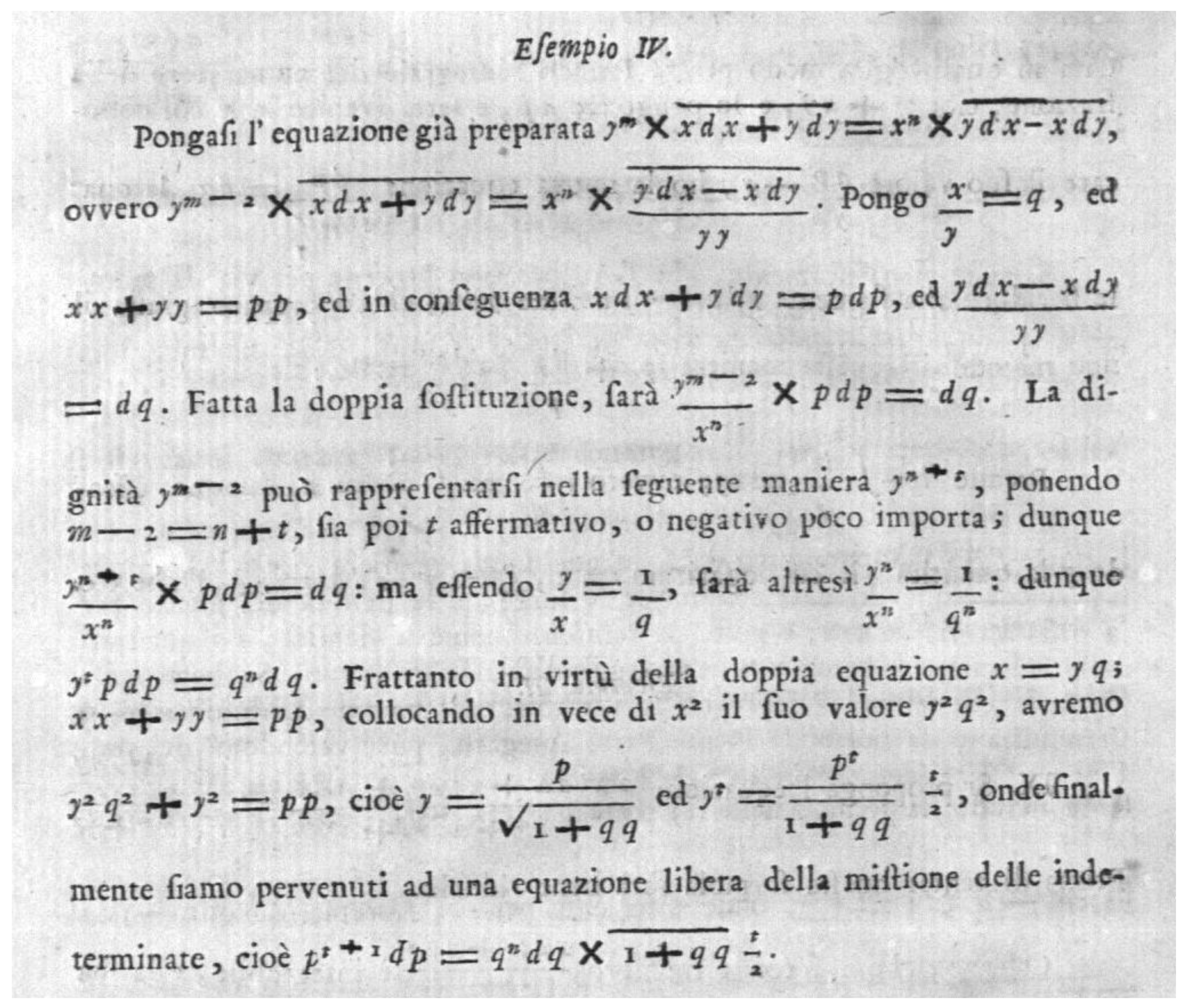
Here follows Riccati’s argument, given in modern terms; the original source, reference [4] page 486, is shown in Figure 1. The strategy is to seek for the primitive of the two differential forms, which appear in (2). The first step consists in writing (2), dividing both sides for $y^2$:

$$y^{m-2}\left(x\mathrm{d}x+y\mathrm{d}y\right)=x^n{\displaystyle \frac{\left(y\mathrm{d}x-x\mathrm{d}y\right)}{y^2}}.$$

(3)

In terms of total diffentential $Df=f_x\mathrm{d}x+f_y\mathrm{d}y$, we can consider Equation (3) using the following identities:

$$D\left(\frac{1}{2}(x^2+y^2)\right)=x\mathrm{d}x+y\mathrm{d}y,D\left(\frac{x}{y}\right)=\frac{y\mathrm{d}x-x\mathrm{d}y}{y^2}.$$

It is, then, natural to introduce the change of variables

$$q=q(x,y)=\frac{x}{y},p=p(x,y)=\sqrt{x^2+y^2}.$$

(4)

To transform Equation (2) via this change of variable, we first write it in normal form:

$$y^{\prime }={\displaystyle \frac{x^{n}y-x{y}^m}{y^{m+1}+x^{n+1}}}.$$

(5)

For $n=m$ (5) obviously reduces to a homogeneous equation, solvable by elementary methods, whose solution is defined by:

$${\int }_{\frac{y_0}{x_0}}^{\frac{y}{x}}\frac{1+u^{n+1}}{u^n(1+u^2)}\mathrm{d}u=ln\frac{x_0}{x}.$$

(6)

We, thus, may assume $m\ne n.$ Therefore, the change of variable (4) leads to the transformed equation

$$\frac{dp}{dq}=\frac{D_x[p(x,y\left(x\right)]}{D_x[q(x,y\left(x\right)]}=\frac{y{\left(x\right)}^2\left(x+y\left(x\right)y^{\prime }\left(x\right)\right)}{\left(y\left(x\right)-x{y}^{\prime }\left(x\right)\right)\sqrt{x^2+y{\left(x\right)}^2}},$$

but, since $y^{\prime }\left(x\right)$ is provided by (5), we obtain:

$$\frac{dp}{dq}=\frac{x^n{y}^{2-m}}{\sqrt{x^2+y^2}}.$$

Expressing the original variables $(x,y)$ in terms of $(p,q),$ that is, inverting (4):

$$x=\frac{pq}{\sqrt{1+q^2}},y=\frac{p}{\sqrt{1+q^2}},$$

we arrive at the transformed equation

$$\frac{dp}{dq}=p^{-m+n+1}{q}^n{\left(1+q^2\right)}^{\frac{m}{2}-\frac{n}{2}-1},$$

(7)

which is separable, so that the integration of (5) is, as a matter of fact, completed.

2.2. Approach via Lie Theory

We skip the computation of the integrals generated by (7) since, in view of solving a more general family of equations, we will integrate (5) using the infinitesimal generator of the Lie group of symmetries associated to (5). This means (see [1] page 30 Equation (2.57)) that, given Equation (1), if we are able to find two functions $\xi (x,y),\eta (x,y)$ verifying the linearized symmetry condition:

$${\eta }_x^{\prime }+\left({\eta }_y^{\prime }-{\xi }_x^{\prime }\right)\omega -{\xi }_x^{\prime }{\omega }^2-\xi {\omega }_x^{\prime }-\eta {\omega }_y^{\prime }=0,$$

(8)

it is possible to obtain the canonical coordinates associated with (5); see for instance [1] (p. 24).

We can formulate the following theorem, which describes the quadrature formula for the solution of the differential Equation (5).

Theorem 1.

If $n,m$ are real numbers such that $n\ne m$ and if $(x_0,y_0)$ lies in the positive quadrant, then the integral curve of (5) which passes for $(x_0,y_0)$ is implicitly defined by:

$$\frac{1}{m-n}\left({\left(x^2+y^2\right)}^{\frac{m-n}{2}}-{\left(x_0^2+y_0^2\right)}^{\frac{m-n}{2}}\right)={\int }_{\frac{x_0}{y_0}}^{\frac{x}{y}}{u}^n{\left(1+u^2\right)}^{\frac{m-n-2}{2}}\mathrm{d}u.$$

(9)

Proof. 

To integrate Equation (5), since we know the Riccati variable transformation, we can use the method indicated in [1] page 26 in order to reconstruct the Lie symmetries when canonical coordinates are given. In our situation we found that, defining

$$\xi (x,y)=\frac{x}{{(x^2+y^2)}^{\frac{m-n}{2}}},\eta (x,y)=\frac{y}{{(x^2+y^2)}^{\frac{m-n}{2}}},$$

(10)

the linearized symmetry condition (8) is satisfied: This is a matter of algebraic computation. We explain the “reverse enginerinng” procedure employed to obtain (10). Following the argument of [1] page 26, if $(X,Y)=\left(X\right(x,y),Y(x,y\left)\right)$ are canonical coordinates for the differential Equation (5), expressing the original variables $(x,y)$ in terms of $(X,Y)$ as $x=f(X,Y)$ and $y=g(X,Y)$ the invariance condition requires that the transformed coordinates must satisfy the following translation property:

$$\left\{\begin{array}{c}\widehat{x}=f(X(x,y),Y(x,y)+\epsilon ),\hfill \\ \widehat{y}=g(X(x,y),Y(x,y)+\epsilon ).\hfill \end{array}\right.$$

(11)

Now, also if it is not the case, we assume for a while the change of variable (4) as canonical, and since for it we have

$$f(X,Y)=\frac{XY}{\sqrt{1+X^2}},g(X,Y)=\frac{Y}{\sqrt{1+X^2}},$$

thus, the expressions in the right hand side in (11) read as:

$$\left\{\begin{array}{c}\widehat{x}=x+{\displaystyle \frac{x\epsilon }{\sqrt{x^2+y^2}}},\hfill \\ \widehat{y}=y+{\displaystyle \frac{y\epsilon }{\sqrt{x^2+y^2}}}.\hfill \end{array}\right.$$

(12)

Differentiating with respect to $\epsilon$ (12) should provide, in case of canonical coordinates, the infinitesimal generator of the Lie symmetries of the differential Equation (5). In our situation from (12) we obtain:

$$\breve{\xi }(x,y)=\frac{x}{\sqrt{x^2+y^2}},\breve{\eta }(x,y)=\frac{y}{\sqrt{x^2+y^2}}.$$

The couple $(\breve{\xi },\breve{\eta })$ misses the linearized symmetry condition (8); in fact, the left hand side of (8) evaluated when $\xi =\breve{\eta }$ and $\eta =\breve{\eta }$ is indeed:

$$\frac{(m-n-1)y^m{x}^n\sqrt{x^2+y^2}}{{\left(y^{m+1}+x^{n+1}\right)}^2}.$$

This means that $(\breve{\xi },\breve{\eta })$ is the infinitesimal generator for (5) only in the particular occurrence $m=n+1$ and, more importantly, gives us the suggestion to look for an infinitesimal generator of the form:

$${\xi }_a(x,y)=\frac{x}{{(x^2+y^2)}^a},{\eta }_a(x,y)=\frac{y}{{(x^2+y^2)}^a},$$

where a is a real parameter which we choose in order to meet condition (8). Thus, evaluating the left hand side of (8) for $({\xi }_a,{\eta }_a),$ we get:

$$\frac{y^m{x}^n(-2a+m-n){\left(x^2+y^2\right)}^{1-a}}{{\left(y^{m+1}+x^{n+1}\right)}^2}.$$

(13)

It is clear that (13) is zero if $m-n-2a=0$ and this explains why (10) is the infinitesimal generator of the Lie group of (5). Hence, using (10) we arrive at the canonical coordinates:

$$X(x,y)=\frac{x}{y},Y(x,y)=\frac{1}{m-n}{(x^2+y^2)}^{\frac{m-n}{2}}.$$

Thus, differential Equation (5) is fully separated in:

$$Y^{\prime }=X^n{\left(X^2+1\right)}^{\frac{1}{2}(m-n-2)}.$$

(14)

Hence, integrating (14), we obtain:

$$Y\left(X\right)={\int }_{X_0}^X{u}^n{(1+u^2)}^{\frac{1}{2}(m-n-2)}\mathrm{d}u+Y_0,$$

(15)

where $X_0=x_0/y_0.$ Formula (9) follows, turning back to the original variables $(x,y)$. □

Remark 1.

Keeping in mind the elementary limit, for $p,q>0$

$$\underset{\epsilon \to 0}{lim}\frac{p^{\frac{\epsilon }{2}}-q^{\frac{\epsilon }{2}}}{\epsilon }=\frac{1}{2}ln\frac{p}{q},$$

we can take the limit for $m-n\to 0$ in (9), obtaining

$$\frac{1}{2}ln\frac{x^2+y^2}{x_0^2+y_0^2}={\int }_{\frac{x_0}{y_0}}^{\frac{x}{y}}{u}^n{\left(1+u^2\right)}^{-1}\mathrm{d}u,$$

which, after some elementary computations, agrees with (6).

3. Results

3.1. Hypergeometric Integrations

In some particular situations it is indeed possible to evaluate the integral at the right hand side of (15) in closed form. To this aim, since some notions and terminology are needed. For the sake of completeness, we recall the integral representation of the Gauss hypergeometric function, which is, as is well known, defined in terms of power series, which converges for $\left|x\right|<1$

$${}_2{\mathrm{F}}_1\left(\left.{\displaystyle \genfrac{}{}{0.0pt}{}{a,b}{c}}\right|x\right):=\sum _{n=0}^{\infty }\frac{{\left(a\right)}_n{\left(b\right)}_n}{{\left(c\right)}_n}\frac{x^n}{n!}.$$

When $\mathrm{Re}\left(a\right)>0,\mathrm{Re}(c-a)>0$ then ${}_2{\mathrm{F}}_1$ can be represented by the integral, see [5] Section 2 Equation (30):

$${}_2{\mathrm{F}}_1\left(\left.{\displaystyle \genfrac{}{}{0.0pt}{}{a,b}{c}}\right|x\right)=\frac{\mathsf{\Gamma }\left(c\right)}{\mathsf{\Gamma }\left(a\right)\mathsf{\Gamma }(c-a)}{\int }_0^1\frac{s^{a-1}{(1-s)}^{c-a-1}}{{(1-sx)}^b}\mathrm{d}s.$$

(16)

Equation (16) provides the analytical continuation of ${}_2{\mathrm{F}}_1$ to the complex plane excluding the half line $(1,\infty );$ in the following we will use this fact. Thus integral (15) can be evaluated in closed form, if the hypotheses of the integral representation (16) are fulfilled.

Theorem 2.

If $n,m$ are real numbers $n\ne m$ and if $n>-1$ for any $(x_0,y_0)$ in the positive quadrant, then the integral curve of (5) which passes for $(x_0,y_0)$ has equation $\mathsf{\Phi }(x,y)=\mathsf{\Phi }(x_0,y_0)$ where:

$$\mathsf{\Phi }(x,y)=\frac{n+1}{m-n}{\left(x^2+y^2\right)}^{\frac{m-n}{2}}-{\left(\frac{x}{y}\right)}^{n+1}{}_2{\mathrm{F}}_1\left(\left.{\displaystyle \genfrac{}{}{0.0pt}{}{\frac{n+1}{2},\frac{n-m+2}{2}}{\frac{n+3}{2}}}\right|-\frac{x^2}{y^2}\right).$$

(17)

Proof. 

If $n>-1$ it is possible to invoke (16); in fact, we express the integral in the right hand side of (15) as

$$\frac{1}{2}\left({\int }_0^{X^2}{u}^{\frac{n-1}{2}}{(1+u)}^{\frac{m-n-2}{2}}\mathrm{d}u-{\int }_0^{X_0^2}{u}^{\frac{n-1}{2}}{(1+u)}^{\frac{m-n-2}{2}}\mathrm{d}u\right)+Y_0.$$

(18)

Notice that we must assume the convergence of the integrand in the origin, which is guaranteed by the assumption $n>-1.$ Then, normalizing the integration intervals with the change of variable $s=X^2\sigma$ and $s=X_0^2\sigma$ in the first and the second integral, respectively, in (18) we use (16), to rewrite (14) as:

$$Y\left(X\right)=\frac{1}{2}\left(\frac{2X^{n+1}}{n+1}{}_2{\mathrm{F}}_1\left(\left.{\displaystyle \genfrac{}{}{0.0pt}{}{\frac{n+1}{2},\frac{n+2-m}{2}}{\frac{n+3}{2}}}\right|-X^2\right)\right.\left.-\frac{2X_0^{n+1}}{n+1}{}_2{\mathrm{F}}_1\left(\left.{\displaystyle \genfrac{}{}{0.0pt}{}{\frac{n+1}{2},\frac{n+2-m}{2}}{\frac{n+3}{2}}}\right|-X_0^2\right)\right)+Y_0.$$

Going back to the original variables, we get Equation (17). □

Remark 2.

Since the argument of ${}_2{\mathrm{F}}_1$ in (17) is strictly negative, and so we operate in the analytic continuation of ${}_2{\mathrm{F}}_1$ itself, function $\mathsf{\Phi }(x,y)$ is well posed in the interior of the first quadrant.

Remark 3.

The hypergeometric structure of (17) allows algebraic implicit solutions of (5) provided that the quantity $(n+2-m)/2$ turns out to be a negative integer, so that the ${}_2{\mathrm{F}}_1$ collapses to a polynomial, that, of course, is strictly connected to the fact that in this case integral (9) is computed in terms of elementary functions. Other solutions of (17) expressible in terms of the elementary transcendental occur for half integer values of $n+1/2$ and $(n+2-m)/2.$ We provide a couple of illustrative examples.

Example 1.

For instance, for $n=2,m=6$ (17) allows algebraic solutions: in fact, the differential equation for $x_0,y_0>0$

$$\left\{\begin{array}{c}{y}^{\prime }={\displaystyle \frac{x^{2}y-x{y}^6}{x^3+y^7}},\hfill \\ y\left(x_0\right)=y_0,\hfill \end{array}\right.$$

has an implicit solution given by:

$$\frac{3}{4}{\left(x^2+y^2\right)}^2-\frac{3x^5+5x^3{y}^2}{5y^5}=\frac{3}{4}{\left(x_0^2+y_0^2\right)}^2-\frac{3x_0^5+5x_0^3{y}_0^2}{5y_0^5}.$$

Of course, in this situation it is possible to represent the integral curves in polynomial form, which in this case for simplicity we took $x_0=y_0=1$:

$$30x^2{y}^7+15y^9-12x^5+15x^4{y}^5-20x^3{y}^2-28y^5=0.$$

Example 2.

If we take $n=2$ and $m=3$ in (17) relation

$${}_2{\mathrm{F}}_1\left(\left.{\displaystyle \genfrac{}{}{0.0pt}{}{\frac{3}{2},\frac{1}{2}}{\frac{5}{2}}}\right|-z\right)=\frac{3}{2z^{3/2}}\left(\sqrt{z(1+z)}-\mathrm{arcsinh}\sqrt{z}\right)$$

comes into play, see [6], http://functions.wolfram.com/07.23.03.2889.01 (accessed on 5 June 2021), so that the solution to

$$\left\{\begin{array}{c}{y}^{\prime }={\displaystyle \frac{x^{2}y-x{y}^3}{x^3+y^4}},\hfill \\ y\left(x_0\right)=y_0,\hfill \end{array}\right.$$

for positive initial data is:

$$\frac{\left(2y^2-x\right)\sqrt{x^2+y^2}}{y^2}+\mathrm{arcsinh}\frac{x}{y}=\frac{\left(2y_0^2-x_0\right)\sqrt{x_0^2+y_0^2}}{y_0^2}+\mathrm{arcsinh}\frac{x_0}{y_0}.$$

If $n>-1$ hypotheses for the integral hypergeometric representation (16) are not fulfilled, but it is still possible, and the second parameter m is chosen suitably to obtain a hypergeometric representation of the solution of (5) as shown in the following Theorem 3.

Theorem 3.

If $n,m$ are real numbers $n\ne m$ such that $n\le -1$ and $m<1$ then for any $(x_0,y_0)$ in the positive quadrant, the integral curve of (5) which passes for $(x_0,y_0)$ has equation $\mathsf{\Xi }(x,y)=\mathsf{\Xi }(x_0,y_0),$ where:

$$\mathsf{\Xi }(x,y)=\frac{1-m}{m-n}{\left(x^2+y^2\right)}^{\frac{m-n}{2}}+{\left(\frac{y}{x}\right)}^{1-m}{}_2{\mathrm{F}}_1\left(\left.{\displaystyle \genfrac{}{}{0.0pt}{}{\frac{1-m}{2},\frac{n-m+2}{2}}{\frac{3-m}{2}}}\right|-\frac{y^2}{x^2}\right).$$

(19)

Proof. 

Since we cannot use the integral representation to evaluate integral (15) we change variable $u=1/v$ so that

$$Y={\int }_{\frac{1}{X}}^{\frac{1}{X_0}}{v}^{-m}{\left(1+v^2\right)}^{\frac{1}{2}(m-n-2)}\mathrm{d}v+Y_0.$$

(20)

At this point, integral (20) can be handled with the same technique used in Theorem 2 to arrive at thesis (19); we omit the computational details here. □

Example 3.

Taking $n=-2,m=-3$ differential Equation (17) becomes

$$\left\{\begin{array}{c}{y}^{\prime }={\displaystyle \frac{y^4-x^3}{x^{2}y+x{y}^3}},\hfill \\ y\left(x_0\right)=y_0,\hfill \end{array}\right.$$

and its solution via (19) is given by:

$$\frac{2x^2-x+y^2}{x\sqrt{x^2+y^2}}=\frac{2x_0^2-x_0+y_0^2}{x_0\sqrt{x_0^2+y_0^2}}.$$

3.2. A More General Equation

The use of the Lie symmetries, until now has not improved what Riccati found, if we leave aside the hypergeometric integration of (14) that was of course unknown in Riccati’s age. However, having a more general perspective enables the discovery of a richer family of differential equations which can be treated with this method. Let $r,s$ be two positive reals and let m and n be two real numbers such that $n\ne m.$ Consider the differential equation in Pfaffian form:

$$y^{m}D\left(\frac{1}{r}(x^r+y^r)\right)=x^n{y}^{s+1}D\left(\frac{x^s}{s{y}^s}\right).$$

(21)

Equation (21) can be written in normal form as

$$y^{\prime }=\frac{x^{n+s-1}y-x^r{y}^m}{y^{m+r}+x^{n+s}}.$$

(22)

We are in position to provide the generalization of Theorem 1.

Theorem 4.

If $n,m,r,$ are real numbers $n+r\ne m+s$ and if $(x_0,y_0)$ lies in the positive quadrant, then the integral curve of (22) which passes for $(x_0,y_0)$ is implicitly defined by:

$$\begin{array}{cc}\hfill & \frac{1}{m-n+r-s}\left({\left(x^{1+r}+y^{1+r}\right)}^{\frac{m-n+r-s}{1+r}}-{\left(x_0^{1+r}+y_0^{1+r}\right)}^{\frac{m-n+r-s}{2}}\right)=\hfill \\ \hfill & {\int }_{\frac{x_0}{y_0}}^{\frac{x}{y}}{u}^{n+s-1}{\left(1+u^{1+r}\right)}^{\frac{m-n-s-1}{2}}\mathrm{d}u.\hfill \end{array}$$

(23)

Proof. 

The thesis follows observing that in this situation the infinitesimal generator of the Lie group of transformation associated at the Equation (22) is

$$\xi (x,y)=\frac{x}{{(x^{r+1}+y^{r+1})}^{\frac{m-n+r-s}{r+1}}},\eta (x,y)=\frac{y}{{(x^{r+1}+y^{r+1})}^{\frac{m-n+r-s}{r+1}}}.$$

(24)

Therefore the canonical coordinates are readily obtained:

$$Y(x,y)=\frac{{(x^{r+1}+y^{r+1})}^{\frac{m-n+r-s}{r+1}}}{m-n+r-s},X(x,y)=\frac{x}{y},$$

and using these coordinates Equation (22) is transformed into:

$$Y^{\prime }=X^{n+s-1}{(1+X^{r+1})}^{\frac{m-n-s-1}{r+1}}.$$

(25)

Equation (23) follows in a similar fashion as Theorem 2 □

Remark 4.

For $r=s=1$ Theorem 4 reduces to Theorem 1.

At this point it is also easy to generalize Theorem 2 using again the integral representation (16).

Theorem 5.

$n,m$ are real numbers $n+r\ne m+s$ and assume:

$$n+s>0.$$

(26)

If $(x_0,y_0)$ lies in the positive quadrant, then the integral curve of (22) for $(x_0,y_0)$ has equation:

$$\mathsf{\Psi }(x,y)=\mathsf{\Psi }(x_0,y_0),$$

(27)

where:

$$\mathsf{\Psi }(x,y)=\frac{n+s}{m-n+r-s}{\left(x^{r+1}+y^{r+1}\right)}^{\frac{m-n+r-s}{1+r}}-{\left(\frac{x}{y}\right)}^{n+s}{}_2{\mathrm{F}}_1\left(\left.{\displaystyle \genfrac{}{}{0.0pt}{}{\frac{n+s}{1+r},\frac{1-m+n+s}{1+r}}{\frac{n+r+s+1}{r+1}}}\right|-\frac{x^{r+1}}{y^{r+1}}\right).$$

(28)

Proof. 

To solve (22) we have to integrate the canonical (fully separated) differential Equation (25) and, as in Theorem 2, in order to express the integral in terms of ${}_2{\mathrm{F}}_1$ we need to extend the integration interval including the origin and so we have to impose conditions (see the right hand side of (23)) $1-n-s<1$ which is ensured by (26). Thus we can adapt the argument of Theorem 2 to rewrite the right hand side of (23) as:

$$\frac{1}{1+r}\left({\int }_0^{X^{1+r}}\frac{u^{\frac{n-r+s-1}{1+r}}}{{(1+u)}^{\frac{n-m+s+1}{r+1}}}\mathrm{d}u-{\int }_0^{X_0^{1+r}}\frac{u^{\frac{n-r+s-1}{1+r}}}{{(1+u)}^{\frac{n-m+s+1}{r+1}}}\mathrm{d}u\right)+Y_0.$$

(29)

Normalizing the intervals of integration on the right hand side of (29), we can use the same argument of Theorem 2 to arrive at (28). □

Example 4.

We take, for instance, $r=2,s=3,m=2,n=3$ and the initial data $x_0=1,y_0=2$ (22) takes the form:

$$\left\{\begin{array}{c}{y}^{\prime }={\displaystyle \frac{x^{5}y-x^2{y}^2}{x^6+y^4}},\hfill \\ y\left(x_0\right)=y_0.\hfill \end{array}\right.$$

Using (27) and (28) we can provide the solution in implicit form, which to the best of our knowledge, is not yet reported in any repertoire and not obtainable via computer algebra:

$$\frac{2x^3+3y^3+y}{y{\left(x^3+y^3\right)}^{2/3}}=\frac{2x_0^3+3y_0^3+y_0}{y_0{\left(x_0^3+y_0^3\right)}^{2/3}},$$

or in algebraic form, for a suitable constant of integration c:

$${\left(2x^3+3y^3+y\right)}^3=c^3{y}^3{\left(x^3+y^3\right)}^2.$$

In the case that integral representation condition (26) is not fulfilled, theorem (5) cannot be invoked, but it is possible, using exactly the same techniques, obtain the analogous of Theorem 3.

Theorem 6.

If $n,m$ are real numbers $n+s\ne m+r$ such that $n\le -s$ and if condition

$$\frac{m+r}{1+r}<1,$$

(30)

then for any $(x_0,y_0)$ in the positive quadrant, the integral curve of (22) which passes for $(x_0,y_0)$ has equation $\mathsf{\Lambda }(x,y)=\mathsf{\Lambda }(x_0,y_0),$ where

$$\begin{array}{cc}\hfill \mathsf{\Lambda }(x,y)& ={\displaystyle \frac{1-m}{m-n+r-s}}{\left(x^{r+1}+y^{r+1}\right)}^{\frac{m-n+r-s}{1+r}}\hfill \\ \hfill & +{\left(\frac{y}{x}\right)}^{1-m}{}_2{\mathrm{F}}_1\left(\left.{\displaystyle \genfrac{}{}{0.0pt}{}{\frac{1-m}{1+r},\frac{n-m+s+1}{1+r}}{\frac{r-m+2}{1+r}}}\right|-\frac{y^{1+r}}{x^{1+r}}\right).\hfill \end{array}$$

(31)

Proof. 

Since in this situation the integrand at the right hand side of (23) is not integrable at the origin we use, as we did in theorem 3, the variable transformation $u=1/v$, obtaining:

$$Y-Y_0=\frac{1}{1+r}{\int }_{\frac{1}{X^{1+r}}}^{\frac{1}{X_0^{1+r}}}\frac{v^{-\frac{m+r}{1+r}}}{{(1+v)}^{\frac{n-m+1+s}{1+r}}}\mathrm{d}v.$$

(32)

Condition (30) ensures the integrability at the origin of (32) and from this point the same hypergeometric integration procedure can be repeated concluding the proof of the theorem. □

Example 5.

Taking $n=-4,m=-2,r=1,s=2$ Equation (22) assumes the form

$$y^{\prime }=\frac{\frac{y}{x^3}-\frac{x}{y^2}}{\frac{1}{x^2}+\frac{1}{y}}=-\frac{x^4-y^3}{x^{3}y+x{y}^2}.$$

From (31) we infer that integral curves through $(x_0,y_0)$ in the first quadrant are:

$$\frac{\left(2x^2+y\right)\sqrt{x^2+y^2}}{x^2}-\mathrm{arcsinh}\left(\frac{y}{x}\right)=\frac{\left(2x_0^2+y_0\right)\sqrt{x_0^2+y_0^2}}{x_0^2}-\mathrm{arcsinh}\left(\frac{y_0}{x_0}\right),$$

Notice that we used the identity:

$${}_2{\mathrm{F}}_1\left(\left.{\displaystyle \genfrac{}{}{0.0pt}{}{\frac{3}{2},\frac{1}{1}}{\frac{5}{2}}}\right|-z\right)=\frac{1}{2}\left(\frac{3\sqrt{1+z}}{z}-\frac{3\mathrm{arcsinh}\sqrt{z}}{z^{\frac{3}{2}}}\right),$$

see [6], http://functions.wolfram.com/HypergeometricFunctions/Hypergeometric2F1/03/07/07/03/0012/ (accessed on 5 June 2021).

4. Discussion

Starting from a two parameter family of differential equations, (5), studied by Jacopo Riccati in the second part of his treatise [4], we interpreted Riccati’s procedure in terms of Lie symmetries, extending it to the more general four parameter family of Equation (22). Once the canonical form of both families of equations has been obtained, see (14) and (25) providing quadrature relations, Theorems 1 and 4, we derive, where possible, through integral representation of Gauss hypergeometric function ${}_2{\mathrm{F}}_1$, the explicit representation of integral curves, Theorems 2, 3, 5 and 6. Finally, some particular cases have been highlighted in which these representations are given in terms of algebraic curves or containing elementary transcendents. Note that none of the particular cases reported in the Examples 1–5 appear in specialistic repertories and are not obtainable via computer algebra. The latter, however, greatly facilitated the search for infinitesimal generators (10) and (24) used in the proofs of Theorems 1 and 4.

5. Conclusions

Hopefully the contribution made in this article is a prelude to further research developments in the field of ordinary differential equations, continuing the historical interpretation approach adopted here, i.e., not limiting it to a chronological description of the results obtained by the founding masters, but rather to mastering their techniques, in the light of both the most recent knowledge, such as Lie symmetries, used in this article, and computer algebra, which allows to tackle computational difficulties that could not be faced previously and to consider generalisations of equations dealt with in the past.

References

- Hydon, P.E. Symmetry Methods for Differential Equations; Cambridge University Press: Cambridge, UK, 2000. [Google Scholar]
- Spiegel, M.R. Applied Differential Equation, 2nd ed.; Prentice-Hall Inc.: Englewood Cliffs, NJ, USA, 1967. [Google Scholar]
- Ritger, P.D.; Rose, N.J. Differential Equation with Applications; Mc Graw Hill: New York, NY, USA, 1968. [Google Scholar]
- Riccati, J. Opere del Conte Jacopo Riccati, Nobile Trevigiano, Tomo I; Appresso J. Giusti: Lucca, Italy, 1761. [Google Scholar]
- Legendre, A.M. Exercices de Calcul Intégral sur Divers Ordres de Transcendantes et Sur Les Quadratures; Courcier: Paris, France, 1811. [Google Scholar]
- Wolfram. The Mathematical Functions Website. Available online: http://functions.wolfram.com (accessed on 5 June 2021).
Figure 1.
Riccati original treatment of (2).
Publisher’s Note: MDPI stays neutral with regard to jurisdictional claims in published maps and institutional affiliations. |
© 2021 by the author. Licensee MDPI, Basel, Switzerland. This article is an open access article distributed under the terms and conditions of the Creative Commons Attribution (CC BY) license (https://creativecommons.org/licenses/by/4.0/).
Share and Cite
MDPI and ACS Style
Ritelli, D. A Forgotten Differential Equation Studied by Jacopo Riccati Revisited in Terms of Lie Symmetries. Mathematics 2021, 9, 1312. https://0-doi-org.brum.beds.ac.uk/10.3390/math9111312
AMA Style
Ritelli D. A Forgotten Differential Equation Studied by Jacopo Riccati Revisited in Terms of Lie Symmetries. Mathematics. 2021; 9(11):1312. https://0-doi-org.brum.beds.ac.uk/10.3390/math9111312
Chicago/Turabian StyleRitelli, Daniele. 2021. "A Forgotten Differential Equation Studied by Jacopo Riccati Revisited in Terms of Lie Symmetries" Mathematics 9, no. 11: 1312. https://0-doi-org.brum.beds.ac.uk/10.3390/math9111312
Note that from the first issue of 2016, this journal uses article numbers instead of page numbers. See further details here.