
Numerical Analysis of Flow Phenomena in Discharge Object with Siphon Using Lattice Boltzmann Method and CFD

 , , , ,
  and
and 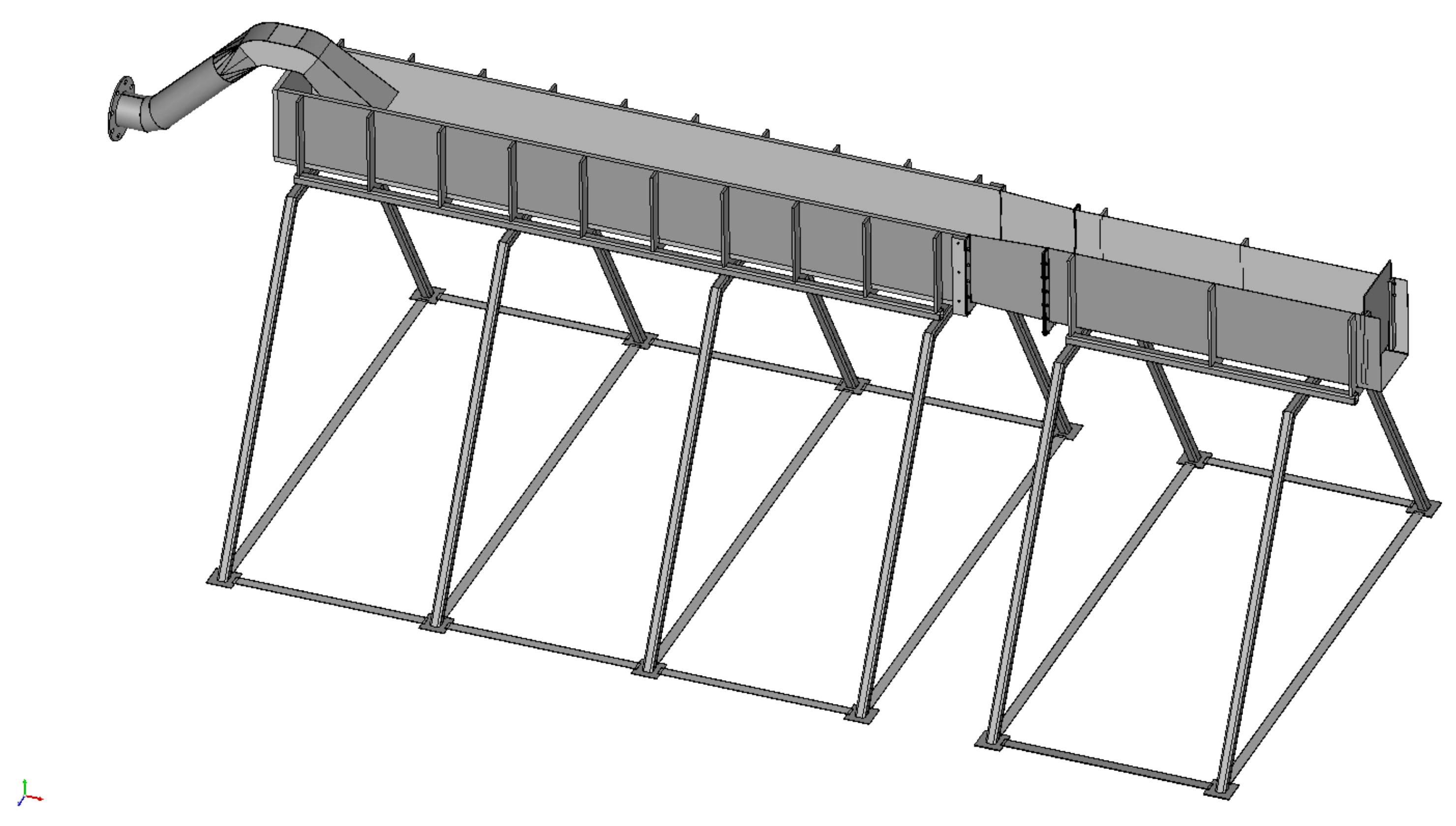
Abstract
:1. Introduction
2. Materials and Methods
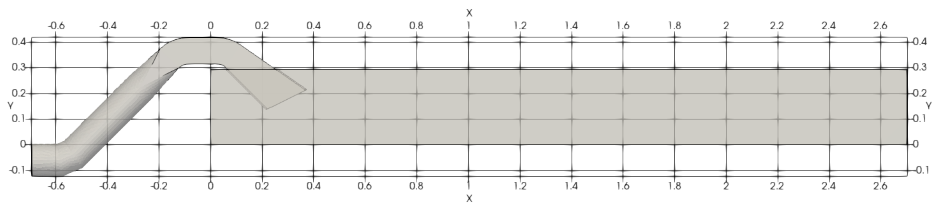
2.1. Formulation of the Problem
2.2. Lattice Boltzmann Method
2.2.1. Free-Surface LBM
2.2.2. Boundary Conditions for Free-Surface LBM
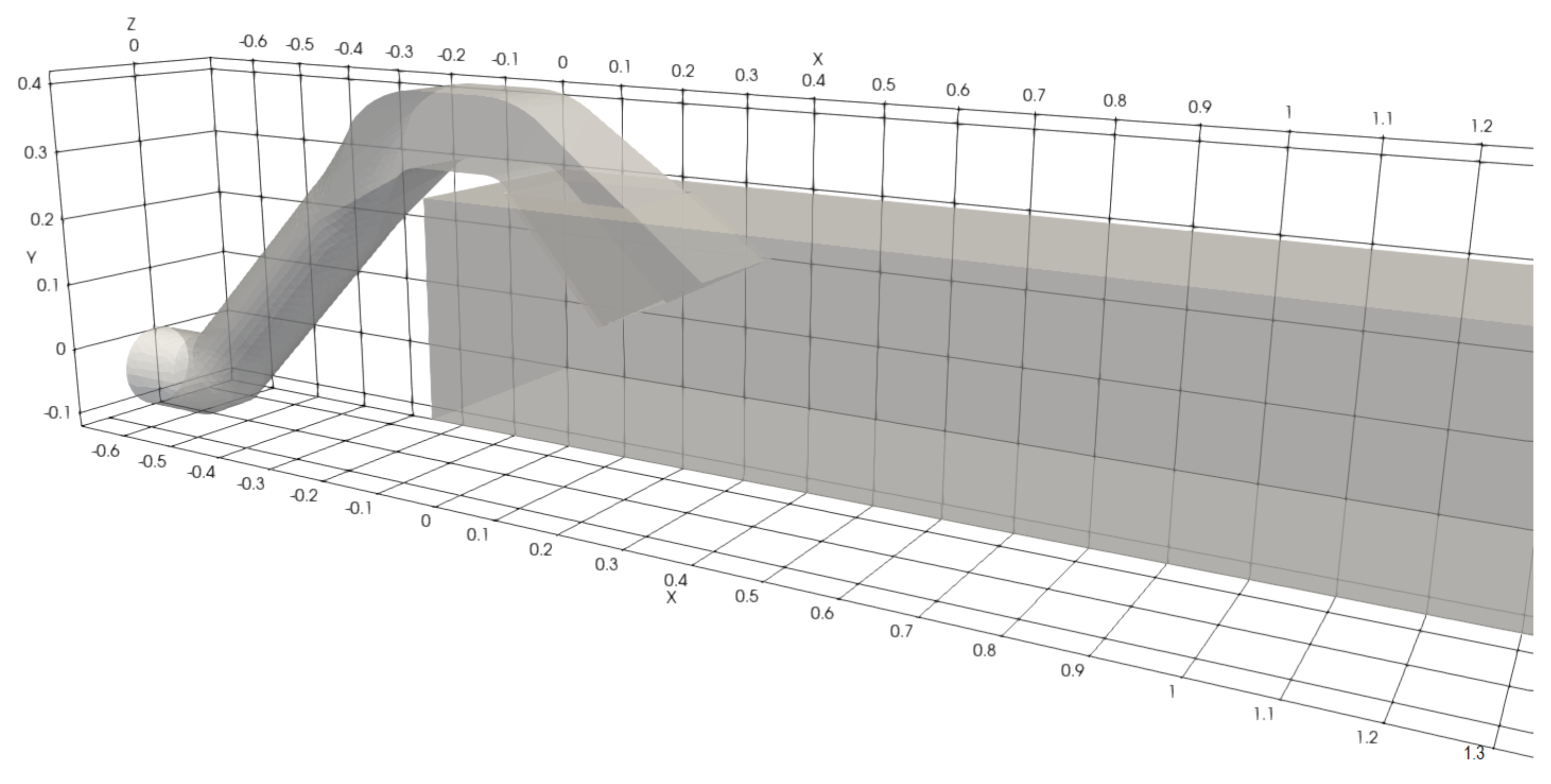
2.2.3. Computational Mesh and Case Setup
2.3. Finite Volume Method
2.4. Experimental Methods
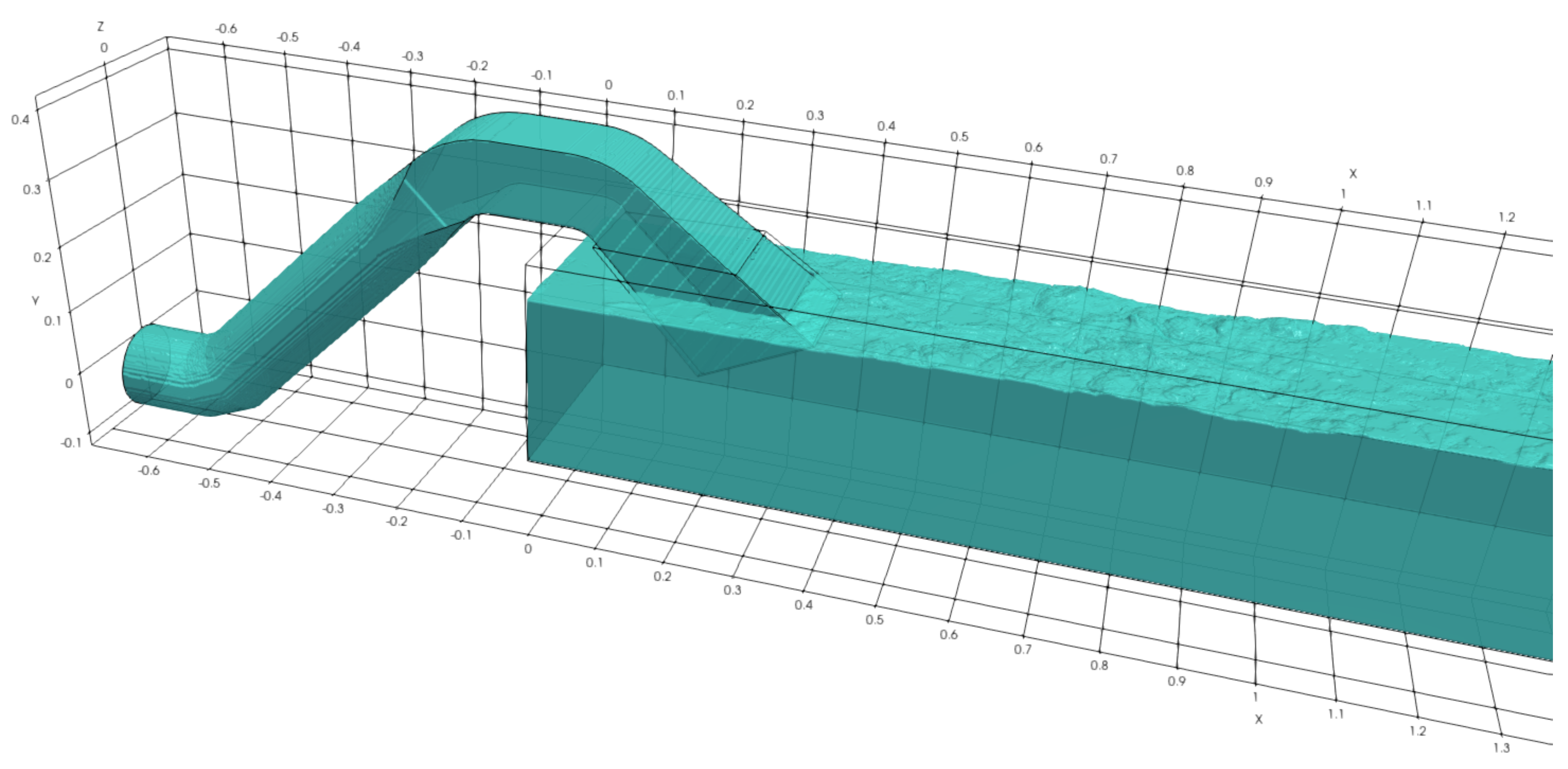
3. Results
4. Discussion
Author Contributions
Funding
Data Availability Statement
Acknowledgments
Conflicts of Interest
References
- Zhu, H.; Zhu, G.; Lu, W.; Zhang, Y. Optimal Hydraulic Design and Numerical Simulation of Pumping Systems. Procedia Eng. 2012, 28, 75–80. [Google Scholar] [CrossRef] [Green Version]
- Sedlář, M.; Procházka, P.; Komárek, M.; Uruba, V.; Skála, V. Experimental Research and Numerical Analysis of Flow Phenomena in Discharge Object with Siphon. Water 2020, 12, 3330. [Google Scholar] [CrossRef]
- Sedlář, M.; Machalka, J.; Komárek, M. Modeling and Optimization of Multiphase Flow in Pump Station. J. Phys. Conf. Ser. 2020, 1584, 012070. [Google Scholar] [CrossRef]
- Queutey, P.; Deng, G.; Wackers, J.; Guilmineau, E.; Leroyer, A.; Visonneau, M. Sliding Grids and Adaptive Grid Refinement for RANS Simulation of Ship-Propeller Interaction. Ship Technol. Res. 2012, 59, 44–57. [Google Scholar] [CrossRef]
- Wackers, J.; Deng, G.; Leroyer, A.; Queutey, P.; Visonneau, M. Adaptive grid refinement for hydrodynamic flows. Comput. Fluids 2012, 55, 85–100. [Google Scholar] [CrossRef]
- McNamara, G.R.; Zanetti, G. Use of the Boltzmann Equation to Simulate Lattice-Gas Automata. Phys. Rev. Lett. 1988, 61, 2332–2335. [Google Scholar] [CrossRef]
- Guo, Z.; Shu, C. Lattice Boltzmann Method and Its Applications in Engineering. In Advances in Computational Fluid Dynamics; World Scientific: Singapore, 2013; Volume 3. [Google Scholar] [CrossRef] [Green Version]
- Du, R.; Wang, J.; Sun, D. Lattice-Boltzmann Simulations of the Convection-Diffusion Equation with Different Reactive Boundary Conditions. Mathematics 2019, 8, 13. [Google Scholar] [CrossRef] [Green Version]
- Yan, G.; Li, Z.; Bore, T.; Torres, S.A.G.; Scheuermann, A.; Li, L. Discovery of Dynamic Two-Phase Flow in Porous Media Using Two-Dimensional Multiphase Lattice Boltzmann Simulation. Energies 2021, 14, 4044. [Google Scholar] [CrossRef]
- Hu, L.; Dong, Z.; Peng, C.; Wang, L.P. Direct Numerical Simulation of Sediment Transport in Turbulent Open Channel Flow Using the Lattice Boltzmann Method. Fluids 2021, 6, 217. [Google Scholar] [CrossRef]
- Ilyin, O. Discrete Velocity Boltzmann Model for Quasi-Incompressible Hydrodynamics. Mathematics 2021, 9, 993. [Google Scholar] [CrossRef]
- Körner, C.; Thies, M.; Hofmann, T.; Thürey, N.; Rüde, U. Lattice Boltzmann Model for Free Surface Flow for Modeling Foaming. J. Stat. Phys. 2005, 121, 179–196. [Google Scholar] [CrossRef]
- Thürey, N.; Rüde, U. Stable free surface flows with the lattice Boltzmann method on adaptively coarsened grids. Comput. Vis. Sci. 2009, 12, 247–263. [Google Scholar] [CrossRef]
- Mohd, N.; Kamra, M.M.; Sueyoshi, M.; Hu, C. Three-dimensional Free Surface Flows Modeled by Lattice Boltzmann Method: A Comparison with Experimental Data. Evergreen 2017, 4, 29–35. [Google Scholar] [CrossRef]
- Purbasari, R.J.; Suryanto, A.; Anam, S. Numerical simulations of dam-break flows by lattice Boltzmann method. In AIP Conference Proceedings 2021; AIP Publishing: Melville, NY, USA, 2018; p. 060027. [Google Scholar] [CrossRef]
- Sato, K.; Koshimura, S. Validation of the MRT-LBM for three-dimensional free-surface flows: An investigation of the weak compressibility in dam-break benchmarks. Coast. Eng. J. 2020, 62, 53–68. [Google Scholar] [CrossRef]
- Bublík, O.; Lobovský, L.; Heidler, V.; Mandys, T.; Vimmr, J. Experimental validation of numerical simulations of free-surface flow within casting mould cavities. Eng. Comput. 2021. [Google Scholar] [CrossRef]
- Janßen, C.F.; Grilli, S.T.; Krafczyk, M. On enhanced non-linear free surface flow simulations with a hybrid LBM–VOF model. Comput. Math. Appl. 2013, 65, 211–229. [Google Scholar] [CrossRef]
- Gunstensen, A.K.; Rothman, D.H.; Zaleski, S.; Zanetti, G. Lattice Boltzmann model of immiscible fluids. Phys. Rev. A 1991, 43, 4320–4327. [Google Scholar] [CrossRef] [PubMed]
- Sudhakar, T.; Das, A.K. Evolution of Multiphase Lattice Boltzmann Method: A Review. J. Inst. Eng. (India) Ser. C 2020, 101, 711–719. [Google Scholar] [CrossRef]
- Shan, X.; Chen, H. Lattice Boltzmann model for simulating flows with multiple phases and components. Phys. Rev. E 1993, 47, 1815–1819. [Google Scholar] [CrossRef] [PubMed] [Green Version]
- Swift, M.R.; Orlandini, E.; Osborn, W.R.; Yeomans, J.M. Lattice Boltzmann simulations of liquid-gas and binary fluid systems. Phys. Rev. E 1996, 54, 5041–5052. [Google Scholar] [CrossRef]
- Zheng, H.; Shu, C.; Chew, Y. A lattice Boltzmann model for multiphase flows with large density ratio. J. Comput. Phys. 2006, 218, 353–371. [Google Scholar] [CrossRef]
- Zou, Q.; Hou, S.; Chen, S.; Doolen, G.D. A improved incompressible lattice Boltzmann model for time-independent flows. J. Stat. Phys. 1995, 81, 35–48. [Google Scholar] [CrossRef]
- Guo, Z.; Zheng, C.; Shi, B. Discrete lattice effects on the forcing term in the lattice Boltzmann method. Phys. Rev. E 2002, 65, 046308. [Google Scholar] [CrossRef] [PubMed]
- Hou, S.; Sterling, J.; Chen, S.; Doolen, G. A lattice Boltzmann subgrid model for high Reynolds number flows. In Pattern Formation and Lattice Gas Automata; American Mathematical Society: Providence, RI, USA, 1995; pp. 151–166. [Google Scholar] [CrossRef]
- Latt, J.; Chopard, B.; Malaspinas, O.; Deville, M.; Michler, A. Straight velocity boundaries in the lattice Boltzmann method. Phys. Rev. E 2008, 77, 056703. [Google Scholar] [CrossRef] [PubMed]
- Donath, S.; Feichtinger, C.; Pohl, T.; Götz, J.; Rüde, U. Localized Parallel Algorithm for Bubble Coalescence in Free Surface Lattice-Boltzmann Method. In Euro-Par 2009 Parallel Processing; Sips, H., Epema, D., Lin, H.X., Eds.; Springer: Berlin/Heidelberg, Germany, 2009; Volume 5704, pp. 735–746. [Google Scholar] [CrossRef]
- Latt, J.; Malaspinas, O.; Kontaxakis, D.; Parmigiani, A.; Lagrava, D.; Brogi, F.; Belgacem, M.B.; Thorimbert, Y.; Leclaire, S.; Li, S.; et al. Palabos: Parallel Lattice Boltzmann Solver. Comput. Math. Appl. 2020. [Google Scholar] [CrossRef]
- Menter, F.R.; Egorov, Y. The Scale-Adaptive Simulation Method for Unsteady Turbulent Flow Predictions. Part 1: Theory and Model Description. Flow Turbul. Combust. 2010, 85, 113–138. [Google Scholar] [CrossRef]
- Menter, F.R.; Kuntz, M.; Langtry, R. Ten Years of Industrial Experience with the SST Turbulence Model. Turbul. Heat Mass Transf. 2003, 4, 625–632. [Google Scholar]
- Nicoud, F.; Ducros, F. Subgrid-scale stress modelling based on the square of the velocity gradient tensor. Flow Turbul. Combust. 1999, 62, 183–200. [Google Scholar] [CrossRef]


Publisher’s Note: MDPI stays neutral with regard to jurisdictional claims in published maps and institutional affiliations. |
© 2021 by the authors. Licensee MDPI, Basel, Switzerland. This article is an open access article distributed under the terms and conditions of the Creative Commons Attribution (CC BY) license (https://creativecommons.org/licenses/by/4.0/).
Share and Cite
Fürst, J.; Halada, T.; Sedlář, M.; Krátký, T.; Procházka, P.; Komárek, M. Numerical Analysis of Flow Phenomena in Discharge Object with Siphon Using Lattice Boltzmann Method and CFD. Mathematics 2021, 9, 1734. https://0-doi-org.brum.beds.ac.uk/10.3390/math9151734
Fürst J, Halada T, Sedlář M, Krátký T, Procházka P, Komárek M. Numerical Analysis of Flow Phenomena in Discharge Object with Siphon Using Lattice Boltzmann Method and CFD. Mathematics. 2021; 9(15):1734. https://0-doi-org.brum.beds.ac.uk/10.3390/math9151734
Chicago/Turabian StyleFürst, Jiří, Tomáš Halada, Milan Sedlář, Tomáš Krátký, Pavel Procházka, and Martin Komárek. 2021. "Numerical Analysis of Flow Phenomena in Discharge Object with Siphon Using Lattice Boltzmann Method and CFD" Mathematics 9, no. 15: 1734. https://0-doi-org.brum.beds.ac.uk/10.3390/math9151734